Locality statistics for anomaly detection in time series of graphs

Abstract

The ability to detect change-points in a dynamic network or a time series of graphs is an increasingly important task in many applications of the emerging discipline of graph signal processing. This paper formulates change-point detection as a hypothesis testing problem in terms of a generative latent position model, focusing on the special case of the Stochastic Block Model time series. We analyze two classes of scan statistics, based on distinct underlying locality statistics presented in the literature. Our main contribution is the derivation of the limiting properties and power characteristics of the competing scan statistics. Performance is compared theoretically, on synthetic data, and on the Enron email corpus. We demonstrate that both statistics are admissible in one simple setting, while one of the statistics is inadmissible in a second setting.

I Introduction

The change-point detection problem in a dynamic network is becoming increasingly prevalent in many applications of the emerging discipline of graph signal processing. Dynamic network data are often readily observed, with vertices denoting entities and time evolving edges signifying relationships between entities, and thus considered as a time series of graphs which is a natural framework for investigation. An anomalous signal is broadly interpreted as constituting a deviation from some normal network pattern, e.g. a model-based characterization such as large scan statistics (c.f. § IV) or non-model based notions such as a community structure change, while a change-point is the time-window during which the anomaly appears.

Recently, many tailor-made approaches based on different models, aiming for change-point detection in graphs, have been proposed in a growing literature. [1] designs a two-stage Bayesian anomaly detection method for social dynamic graphs. Both its model and parallelization in computation are built on the assumption that the communication between each pair of individuals independently follows a counting process. In [2], an algorithm called NetSpot is created to find arbitrary but evolutionary anomalies that are maintained over a spatial or time window, i.e., the anomalous signal does not appears and then disappears instantaneously In [3], the subgraph anomaly detection problem in static graphs were analyzed through likelihood ratio tests under a Poisson random graph model. Finally, in [4], the $L_{1}$ norm of the eigenvectors of the modularity matrix were used for detection of an (anomalous) small dense subgraph embedded inside a large, sparser graph.

In this paper, we approach the dynamic anomaly/change-point detection problem through the use of locality-based scan statistics. Scan statistics are commonly used in signal processing to detect a local signal in an instantiation of some random field [5, 6]. The idea is to scan over a small time or spatial window of the data and calculate some locality statistic for each window. The maximum of these locality statistics is known as the scan statistic. Large values of the scan statistic suggests existence of nonhomogeneity, for example, a local region with significantly excessive communications. Under some homogeneity hypothesis, change-point detection can then be reduced to statistical hypotheses testing (c.f. § III) using scan statistics. For example, [7] builds up a simple testing framework with the null hypothesis being Erdös-Rényi and the alternative hypothesis being a graph containing an unusually dense subgraph. In the static graph setting, detection boundaries and conditions are given in [7] such that the scan statistics they specified for the testing is non-negligibly powerful. To capture anomalies (e.g. hacker attacks) in computer networks, [8] employs scan statistics through two shapes of locality statistics: ’star’ and ’k-path’. The power properties of ’star’ as a locality measure will be further explored in § V here.

In this paper, we identify excessive communication activity in a subregion of a dynamic network by employing the scan statistics $S_{\tau,\ell,k}(t;\cdot)$ defined in § IV, with $\tau$ denoting the number of vertex-standardization steps, $\ell$ denoting the number of temporal-normalization steps and $k$ denoting local neighborhood distance. We consider two variations of $S_{\tau,\ell,k}(t;\cdot)$, namely $S_{\tau,\ell,k}(t;\Psi)$ and $S_{\tau,\ell,k}(t;\Phi)$ where $\Psi$ and $\Phi$ are two related but distinct locality statistics. The use of the locality statistics $\Psi$ and $\Phi$ is based upon earlier work of [9] and [10]. In particular, $\Psi$ is introduced in [9] to detect the emergence of local excessive activities in time series of Enron graphs whereas $\Phi$ is proposed in [10] to detect communication pattern changes in their department email network. Using the locality statistic $\Psi$, [11] constructs fusion statistics of graphs for anomaly detection while [12] presents an analysis of the Enron data set to illustrate statistical inference for attributed random graphs. However, all these cited works are mostly empirical in nature and do not provide much theoretical analysis of these locality-based scan statistics. Under the assumption that the time series of graphs is stationary before a change-point, we demonstrate in this paper that for $\tau=1$ and $\ell=0$, the limiting $S_{\tau,\ell,k}(t;\Psi)$ and $S_{\tau,\ell,k}(t;\Phi)$ are the maximum of random variables which, under proper normalizations, follow a standard Gumbel $\mathcal{G}(0,1)$ distribution in the limit. Through these limiting properties, comparative power analysis between $S_{\tau,\ell,k}(t;\Psi)$ and $S_{\tau,\ell,k}(t;\Phi)$ for $\tau=1$ and $\ell=0$ is performed We demonstrate that both $\Psi$ and $\Phi$ are admissible if $k=0$, while $\Psi$ is inadmissible if $k=1$. We hope that these theoretical results will help motivate subsequent work in understanding the interplay between locality statistics, vertex and temporal normalizations, and inference in time-series of graphs.

Our paper is structured as follows. We discuss a generative model for time series of graphs in § II. The problem of change-point detection is formulated in § III. The formulation associates a change-point in the time series with changes in the underlying generative model. We introduce in § IV two closely related notions of locality statistic, $\Psi$ and $\Phi$, and their corresponding scan statistics $S_{\tau,\ell,k}(t;\Psi)$ and $S_{\tau,\ell,k}(t;\Phi)$. The limiting properties and power characteristics for some representative instances of $S_{\tau,\ell,k}(t;\cdot)$ are given in § V and VI, while § VII presents experimental results regarding locality-based statistics on synthetic data and the Enron email corpus. We conclude the paper in § VIII with additional discussions of the two locality statistics and comments about possible applications and extensions of the framework presented herein.

I-A Notation

We introduce some notation that will be used throughout this paper. In this paper, we consider only undirected and unweighted graphs without self-loops. Generally, a graph is denoted by $G$, with vertex set $V=V(G)$ and edge set $E=E(G)$. The number of vertices of a graph is usually denoted by $n$. For a graph $G$ on $n$ vertices, the vertex set is usually taken to correspond to the set $[n]=\{1,2,\dots,n\}$. In our subsequent discussion, we might also partition $V$ into subsets, or blocks. If $V$ is partitioned into $B$ blocks of size $n_{1},n_{2},\dots,n_{B}$ vertices, then, with a slight abuse of notation, we shall denote by $[n_{i}]$ the vertices in block $i$.

Let $G$ be a graph. For any $u,v\in V$, we write $u\sim v$ if there exists an edge between $u$ and $v$ in $G$. We write $d(u,v)$ for the shortest path distance between $u$ and $v$ in $G$. For $v\in V$, we denote by $N_{k}[v;G]$ the set of vertices $u$ at distance at most $k$ from $v$, i.e., $N_{k}[v;G]=\{u\in V\colon d(u,v)\leq k\}$. For $V^{\prime}\subset V$, $\Omega(V^{\prime},G)$ is the subgraph of $G$ induced by $V^{\prime}$. Thus, $\Omega(N_{k}[v;G],G)$ is the subgraph of $G$ induced by vertices at distance at most $k$ from $v$.

II Random graph models

In this section, we briefly summarize the latent position model of [13], the dot product model of [14] and stochastic blockmodel of [15] and [16], since they are the underlying generative model for our graph $G_{t}$ at each time $t$.

The latent position model is motivated by the assumption that each vertex $v$ is associated with a $K$ dimensional latent random vector $X_{v}$. For any pair of vertices $u$ and $v$, conditioning on the two latent positions $X_{u}$ and $X_{v}$, the existence of an edge between $u$ and $v$ is independently determined by a Bernoulli trial with probability $f(X_{u},X_{v})$ where $f$ is a symmetric link function $f:\mathbb{R}^{K}\times\mathbb{R}^{K}\to[0,1]$. Namely, $\mathbf{1}_{\{u\sim v\}}\stackrel{{\scriptstyle ind}}{{\sim}}Bernoulli(f(X_{u},X_{v}))$.

The random dot product graph model (RDPM) [14] is a special case of the latent position model. In the random dot product graph model, the link function $f$ is specified to be the Euclidean inner product, i.e., $f(X_{u},X_{v})=\langle X_{u},X_{v}\rangle$. Also, for each vertex $v$, the latent random vector $X_{v}$ takes its values in the unit simplex $\mathscr{S}$ so that $0\leq\langle X_{u},X_{v}\rangle\leq 1$ where

$$\mathscr{S}=\{x\in[0,1]^{K}:\sum_{k=1}^{K}x_{k}\leq 1\}.$$

The stochastic block model (SBM) of [15] and [16] is a random graph model in which each vertex is randomly assigned a block membership among $\{1,\dots,B\}$ where $B$ is the number of blocks. Given block memberships, the connectivity probabilities among all vertices are characterized by a $B\times B$ symmetric matrix $\mathbf{P}$ where $\mathbf{P}_{j,k}$ denotes the block connectivity probability between blocks $j$ and $k$. Namely, $\mathbf{1}_{\{u\sim v\}}\stackrel{{\scriptstyle ind}}{{\sim}}Bernoulli(\mathbf{P}_{j,k})$ given $u\in[n_{j}]$ and $v\in[n_{k}]$.

In this paper, we shall assume that the time series of random graphs $\{G_{t}\}$ are generated according to a stochastic block model where the block membership of the vertices are fixed across time while the connectivity probabilities matrix $\mathbf{P}=\mathbf{P}_{t}$ may varies with time (c.f. our formulation of the change-point detection problem in § III). That is to say, at some initial time, say $t_{0}=0$, we randomly assign each vertex to a block membership among $\{1,2,\dots,K\}$. Then at each subsequent time $t\geq t_{0}$, $G_{t}$ follows a SBM with a $K\times K$ probability matrix $\mathbf{P}_{t}$, conditioned on the initial block membership at time $t_{0}$. Under this model, the graphs are conditionally independent over time, the conditioning being on the block membership of the vertices. This assumption on the generative model for the $\{G_{t}\}$ leads to a time series of graphs where the graphs are “weakly” dependent, i.e., they are dependent only on the block membership of the vertices at the initial time $t_{0}$. If, instead, for each time $t$, we resample the vertices’ block membership for $G_{t}$ then the resulting time series of graphs is independent.

Our construction of a time series of graphs in terms of the SBM as outlined above is a special case of the following model constructed using the random dot product graphs .

1. For each $v\in[n]$ and $t\in\mathbb{N}$,

   $$X_{v}(t)\sim\mathrm{Dirichlet}(r_{v}\vec{\alpha}_{v}+\vec{1}).$$

2. For each $t\in\mathbb{N}$ and pair of vertices $(u,v)$,

   $$P(u\sim v|\,\mathbf{X}(t))=\langle X_{u}(t),X_{v}(t)\rangle.$$

where $\vec{\alpha}_{v}\in\mathscr{S}$ is a fixed location parameter for the Dirichlet distribution and $r_{v}$ is the concentration parameter that will be explained now.

It is worthwhile to note that $r_{v}=0$ for all $v\in[n]$ means all vertices follow the same probabilistic behavior (uniform on the simplex) and $\min r_{v}\to\infty$ implies that $X_{v}(t)$ has a point mass distribution at $\vec{\alpha}_{v}$ for each vertex. In the case $\min r_{v}\to\infty$, the random dot product model can be further reduced to the stochastic block model (SBM) by letting vertices sharing the same $\vec{\alpha}_{v}$ share the same block membership. Next, we re-denote by $\vec{\alpha}_{i}$ the common Dirichlet location parameter corresponding to block $[n_{i}]$ and $V$ is partitioned into $B$ distinct blocks $[n_{1}],\dots,[n_{B}]$ if there are $B$ distinct $\vec{\alpha}_{i}$’s in total. Accordingly, as $\min r_{i}\to\infty$, $P(u\sim v|\,u\in[n_{j}],v\in[n_{k}])\to\langle\vec{\alpha}_{j},\vec{\alpha}_{k}\rangle$. We note that the above Dirichlet can be viewed as generating a time-series of graphs where the graphs are also “weakly” dependent, e.g., dependency between graphs at time $t$ and $t^{\prime}$ being on the location and concentration parameters $\{(\alpha_{v},r_{v})\}$ for the vertices. Other generalizations of the above construction for generating time series of graphs are also possible. See, e.g., [17] and [18] for examples of constructions where the time series of graphs depends on some underlying latent stochastic processes.

III Change-point detection problem in Stochastic Block model formulation

An important inference task in time series analysis is the problem of anomaly or change-point detection. An anomaly is broadly interpreted to mean deviation from a “normal” pattern and a change-point is the time-window during which the anomalous deviation occurs. For example, in social networks, we usually represent a time-evolving collection of emails, phone calls, web pages visits, etc. as a time series of graphs $\{G_{t}\}$ and we want to infer, from $\{G_{t}\}$, if there exists anomalous activities, e.g., excessive phone calls among a subgroup in the network. In the detection problem described below in § III and its theoretical analysis presented in § V and § VI, we shall implicitly assume, for ease of exposition, that the $\{G_{t}\}$ are independent. As we pointed out in our discussion of the generative model for time-series of graphs in § II, this independence corresponds to conditioning on the right parameters. In the setup of our theoretical analysis in this paper, this corresponds to conditioning on the block membership of the vertices, which are fixed in time. Related discussions in the context of the latent process models of [17] and [18] are given in § VIII.

Statistically speaking, we want to test, for an unknown but non-random $t\in\mathbb{N}$, the null hypothesis $H_{0}$ that $t$ is not a change-point against the alternative hypothesis $H_{A}$ that $t$ is a change-point. There are many different ways to formulate the notion that $t$ is a change-point. The following formulation, in the contex of our discussion, is reasonable and sufficiently general and forms the basis of our subsequent investigation.

We say that $t^{*}$ is a change-point for $\{G_{t}\}$ if there exists distinct choices of $\mathbf{P}^{0}$, $\mathbf{P}^{A}$ independent of $t$ such that

$$H_{A}:G_{t}\sim\begin{cases}\mathrm{SBM}(\mathbf{P}^{0},\{[n_{i}]\})&\text{for $t\leq t^{\ast}-1$}\\ \mathrm{SBM}(\mathbf{P}^{A},\{[n_{i}]\})&\text{for $t\geq t^{\ast}$}\\ \end{cases},$$

where $\mathrm{SBM}(\mathbf{P},\{[n_{i}]\})$ denote the stochastic blockmodel with block connectivity probabilities $\mathbf{P}$ and unknown, but fixed in time, block memberships $\{[n_{i}]\}$. In contrast, the null hypothesis, i.e. the nonexistence of change-point, is

$$H_{0}:G_{t}\sim\mathrm{SBM}(\mathbf{P}^{0},\{[n_{i}]\})~{}\text{for all $t$}.\\$$

That is to say, under the alternative, at time $t^{*}$, a subset of the vertices change their behavior. The vertices whose behaviour changes correspond to the vertices with block memberships whose corresponding rows in the connectivity matrix changes, i.e., from $\mathbf{P}^{0}$ to $\mathbf{P}^{A}$. As permutation of the vertex block labels does not affect our subsequent analysis, we will refer to $(t^{*},\{[n_{i}]\},\mathbf{P}^{0},\mathbf{P}^{A})$ as the change parameters. As a convention, if $t^{\ast}=\infty$, we assume all vertices follow their original dynamics for all $t$.

In the following, we discuss a specific form for $\mathbf{P}^{0}$ and $\mathbf{P}^{A}$, illustrating, albeit in an exaggerated manner, the chatter anomaly, i.e., a subset of vertices with altered communication behavior in an otherwise stationary setting.

$$\mathbf{P}^{0}=\left(\begin{array}[]{ccccc}p_{1}&p_{1,2}&\dots&\dots&p_{1,B}\\ p_{2,1}&h_{2}&\ddots&&\vdots\\ \vdots&\ddots&\ddots&\ddots&\vdots\\ \vdots&&\ddots&h_{B-1}&p_{B-1,B}\\ p_{B,1}&\dots&\dots&p_{B,B-1}&p_{B}\\ \end{array}\right),$$ (1)

$$\mathbf{P}^{A}=\left(\begin{array}[]{ccccc}p_{1}&p_{1,2}&\dots&\dots&p_{1,B}\\ p_{2,1}&h_{2}&\ddots&&\vdots\\ \vdots&\ddots&\ddots&\ddots&\vdots\\ \vdots&&\ddots&h_{B-1}&p_{B-1,B}\\ p_{B,1}&\dots&\dots&p_{B,B-1}&p_{B}+\delta\\ \end{array}\right),$$ (2)

for some $\delta>0$, with $n_{1},n_{2},\dots,n_{B}$ being of size

$$(n_{1},n_{2},\dots,n_{B})=(\Theta(n),O(n),\dots,O(n)).$$

For this form of $\mathbf{P}^{0}$ and $\mathbf{P}^{A}$, the blocks have their own (possibly distinct) self-connectivity probabilities which are diagonal entries of matrices. In other words, before the change-point, each of the blocks $i=2$ up to $B-1$ have self-connectivity probability $h_{i}$. The block $i=1$ is of size $\Theta(n)$ with self-connectivity probability $p_{1}$, representing the probabilistic behaviors of the vast majority of actors in a very large network. The case where $h_{2}>p_{1},\dots,h_{B-1}>p_{1}$ is of interest because we can consider each of the $[n_{i}]$ as representing a “chatty” group for time $t\leq t^{\ast}-1$, and at $t^{\ast}$, the previously non-chatty group $[n_{B}]$ becomes more chatty. See Figure 1 for a notional depiction of $\mathbf{P}^{0}$ and $\mathbf{P}^{A}$ for the case of $B=3$ blocks with $p_{1}=p_{3}=p_{1,2}=p_{1,3}=p_{2,3}=p$. The detection of this transition for the vertices in $[n_{B}]$ is one of the main reasons behind the locality statistics that will be introduced in § IV.

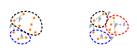
Figure 1: Notional depiction of $\mathbf{P}^{0}$ and corresponding $\mathbf{P}^{A}$. $\mathbf{P}^{0}$: all vertices connect with probability $p$ except that the self-connectivity probability of $[n_{2}]$ is $h$; $\mathbf{P}^{A}$: the self-connectivity probability of $[n_{3}]$ transitions from $p$ to $p+\delta$ while $[n_{2}]$ retains its previous behavior.

IV Locality statistics for change-point detection in time series of graphs

IV-A Two locality statistics

Suppose we are given a time series of graphs $\{G_{t}\}_{t\geq 1}$ where $V(G_{t})$ is independent of $t$, i.e., the graphs $G_{t}$ are constructed on the same vertex set $V$. We now define two different but related locality statistics on $\{G_{t}\}$. For a given $t$, let $\Psi_{t;k}(v)$ be defined for all $k\geq 1$ and $v\in V$ by

$$\Psi_{t;k}(v)=|E(\Omega(N_{k}(v;G_{t});G_{t}))|.$$ (3)

$\Psi_{t;k}(v)$ counts the number of edges in the subgraph of $G_{t}$ induced by $N_{k}(v;G_{t})$, the set of vertices $u$ at a distance at most $k$ from $v$ in $G_{t}$. In a slight abuse of notation, we let $\Psi_{t;0}(v)$ denote the degree of $v$ in $G_{t}$. The statistic $\Psi_{t}$ was first introduced in [9]. [19] investigated the use of $\Psi_{t}$ in analyzing the Enron data corpus.

Let $t$ and $t^{\prime}$ be given, with $t^{\prime}\leq t$. Now define $\Phi_{t,t^{\prime};k}(v)$ for all $k\geq 1$ and $v\in V$ by

$$\Phi_{t,t^{\prime};k}(v)=|E(\Omega(N_{k}(v;G_{t});G_{t^{\prime}}))|.$$ (4)

The statistic $\Phi_{t,t^{\prime};k}(v)$ counts the number of edges in the subgraph of $G_{t^{\prime}}$ induced by $N_{k}(v;G_{t})$.

Once again, with a slight abuse of notation, we let $\Phi_{t,t^{\prime};0}(v)$ denote the degree of $v$ in $G_{t}\cap G_{t^{\prime}}$, where $G\cap G^{\prime}$ for $G$ and $G^{\prime}$ with $V(G)=V(G^{\prime})$ denotes the graph $(V(G),E(G)\cap E(G^{\prime}))$. The statistic $\Phi_{t,t^{\prime};k}(v)$ is motivated by a statistic named the permanent window metric introduced in [20]. The permanent window metric was meant to capture events involving not just a single individual but the whole community. As the community at time $t$ is assumed to be approximated by $N_{k}(v;G_{t})$, the statistic $\Phi_{t,t^{\prime};k}(v)$ uses the community structure at time $t$ in its computation of the locality statistic at time $t^{\prime}\leq t$. Through this measure, a community structure shift of $v$ can be captured even when the connectivity level of $v$ remains unchanged across time, i.e., when the $\Psi_{t}$ stays mostly constant as $t$ changes in some interval. With the purpose of determining whether $t$ is a change-point, two kinds of normalizations based on past $\Psi$ and $\Phi$ locality statistics and their corresponding normalized scan statistics are introduced in the next subsection.

IV-B Temporally-normalized statistics

Let $J_{t,t^{\prime};k}$ be either the locality statistic $\Psi_{t^{\prime};k}$ in Eq. (3) or $\Phi_{t,t^{\prime};k}$ in Eq. (4), where for ease of exposition the index $t$ is a dummy index when $J_{t,t^{\prime};k}=\Psi_{t^{\prime};k}$. We now define two normalized statistics for $J_{t,t^{\prime};k}$, a vertex-dependent normalization and a temporal normalization. These normalizations and their use in the change-point detection problem are depicted in Figure 2.

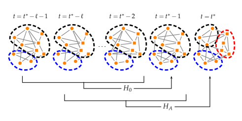
Figure 2: Temporal standardization: when testing for change at time $t$, the recent past graphs $G_{t},G_{t-1},\dots$ are used to standardize the invariants.

For a given integer $\tau\geq 0$ and $v\in V$, we define the vertex-dependent normalization $\widetilde{J}_{t,\tau;k}(v)$ of $J_{t,t^{\prime};k}(v)$ by

$$\widetilde{J}_{t;\tau,k}(v)=\begin{cases}J_{t,t;k}(v)&\tau=0\\ J_{t,t;k}(v)-\hat{\mu}_{t;\tau,k}(v)&\tau=1\\ (J_{t,t;k}(v)-\hat{\mu}_{t;\tau,k}(v))/\hat{\sigma}_{t;\tau,k}&\tau>1\end{cases},$$ (5)

where $\mu_{t;\tau,k}$ and $\sigma_{t;\tau,k}$ are defined as

$$\hat{\mu}_{t;\tau,k}(v)=\frac{1}{\tau}\sum_{s=1}^{\tau}J_{t,t-s;k}(v),$$ (6)

$$\hat{\sigma}_{t;\tau,k}(v)=\sqrt{\frac{1}{\tau-1}\sum_{s=1}^{\tau}{(J_{t,t-s;k}(v)-\hat{\mu}_{t;\tau,k}(v))^{2}}}.$$ (7)

We then consider the maximum of these vertex-dependent normalizations for all $v\in V$, i.e., we define a $M_{\tau,k}(t)$ by

$$M_{\tau,k}(t)=\max_{v}(\widetilde{J}_{t,\tau;k}(v)).$$ (8)

We shall refer to $M_{\tau,0}(t)$ as the standardized max-degree and to $M_{\tau,1}$ as the standardized scan statistics. From Eq. (5), we see that the motivation behind vertex-dependent normalization is to standardize the scales of the raw locality statistics $J_{t,t^{\prime};k}(v)$. Otherwise, in Eq. (8), a noiseless vertex in the past who has dramatically increasing communications at the current time $t$ would be inconspicuous because there might exist a talkative vertex who keeps an even higher but unchanged communication level throughout time.

Finally, for a given integer $l\geq 0$, we define the temporal normalization of $M_{\tau,k}(t)$ by

$$S_{\tau,\ell,k}(t)=\begin{cases}M_{\tau,k}(t)&\ell=0\\ M_{\tau,k}(t)-\tilde{\mu}_{\tau,\ell,k}(t)&\ell=1\\ (M_{\tau,k}(t)-\tilde{\mu}_{\tau,\ell,k}(t))/\tilde{\sigma}_{\tau,\ell,k}(t)&\ell>1\end{cases},$$ (9)

where $\tilde{\mu}_{\tau,\ell,k}$ and $\tilde{\sigma}_{\tau,\ell,k}$ are defined as

$$\tilde{\mu}_{\tau,\ell,k}(t)=\frac{1}{\ell}\sum_{s=1}^{\ell}M_{\tau,k}(t-s),$$ (10)

$$\tilde{\sigma}_{\tau,\ell,k}(t)=\sqrt{\frac{1}{\ell-1}\sum_{s=1}^{\ell}{(M_{\tau,k}(t-s)-\tilde{\mu}_{\tau,\ell,k}(t))^{2}}}.$$ (11)

The motivation behind temporal normalization, based on recent $\ell$ time steps, is to perform smoothing for the statistics $M_{\tau,k}$, similar to how smoothing is performed in time series analysis. Large values of the smoothed statistic indicates an anomaly where there is an excessive increase in communications among a subset of vertices. We will use these $S_{\tau,\ell,k}$ as the test statistics for the change-point detection problem described in § III.

We note that because $\Psi_{t;k}(v)=\Phi_{t,t;k}(v)$ for $M_{\tau,k}$ when $\tau=0$, the choice of locality statistic for $J_{t,t^{\prime};k}$ does not matter when $\tau=0$. For convenience of notation, since $S_{\tau,\ell,k}(t)$ is essentially a function of the $J_{t,t^{\prime};k}$, we denote by $S_{\tau,\ell,k}(t;\Psi)$ and $S_{\tau,\ell,k}(t;\Phi)$ the $S_{\tau,\ell,k}(t)$ when the underlying statistic $J_{t,t^{\prime};k}$ is $\Psi_{t^{\prime};k}$ and $\Phi_{t,t^{\prime};k}$, respectively.

After the above introduction of the temporally-normalized statistics $S_{\tau,\ell,k}(t;\cdot)$ with three parameters $\tau,\ell,k$ , we now present a simple toy example to illustrate a key step in the calculation of $S_{\tau,\ell,k}(t;\cdot)$, namely the calculation of the vertex-dependent normalization $\widetilde{J}_{t;\tau,k}(v)$ presented in Eq. (5). In Figure 3, the table calculates $\widetilde{J}_{t^{\ast};\tau,k}(v)$, when $\tau=1$ and $v=e$, for different underlying statistics $J_{t,t^{\prime};k}$ and different values of $k$. More concretely, because $\tau=1$, $\widetilde{J}_{t^{\ast};1,k}(e)=\Psi_{t^{\ast};k}(e)-\Psi_{t^{\ast}-1;k}(e)$ if the underlying statistic is $\Psi_{t;k}(e)$ and $\widetilde{J}_{t^{\ast};1,k}(e)=\Phi_{t^{\ast},t^{\ast};k}(e)-\Phi_{t^{\ast},t^{\ast}-1;k}(e)$ if the underlying statistic is $\Phi_{t,t^{\prime};k}(e)$.

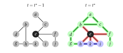
	$J^{k}_{t^{*},t^{*}}(e)$		$\widehat{\mu}^{k}_{t^{*},\tau}(e)$		$\widetilde{J}^{k}_{t^{*},\tau}(e)$
	$k=0$	$k=1$	$k=0$	$k=1$	$k=0$	$k=1$
$\Psi_{t^{\prime};k}$	5	7	3	3	2	4
$\Phi_{t,t^{\prime};k}$	5	7	2	4	3	3

Figure 3: An example to differentiate the calculation of $\widetilde{J}_{t^{\ast};\tau,k}(v)$ with varying underlying statistics ($\Psi_{t;k}$ or $\Phi_{t,t^{\prime};k}$) and order distances ($k=0$ or $k=1$). In the right graph $G_{t^{\ast}}$, note that the red edges are $E(\Omega(N_{k=0}[e;G_{t^{\ast}}],G_{t^{\ast}}))$; the red and blue edges are $E(\Omega(N_{k=1}[e;G_{t^{\ast}}],G_{t^{\ast}}))$; the red, blue and green edges are $E(\Omega(N_{k=2}[e;G_{t^{\ast}}],G_{t^{\ast}}))$. For instance, the magenta-marked number $3$ is $\Psi_{t^{\ast}-1;0}$ where $\Psi_{t^{\ast}-1;0}(e)=|E(\Omega(N_{0}(e;G_{t^{\ast}-1});G_{t^{\ast}-1}))|$ and $E(\Omega(N_{0}(e;G_{t^{\ast}-1});G_{t^{\ast}-1}))=\{e\sim c,e\sim f,e\sim i\}$ in $G_{t^{\ast}-1}$.;the orange-marked number $4$ is $\Phi_{t^{\ast},t^{\ast}-1;1}(e)$ where $\Phi_{t^{\ast},t^{\ast}-1;1}(e)=|E(\Omega(N_{1}(e;G_{t^{\ast}});G_{t^{\ast}-1}))|$ and $E(\Omega(N_{1}(e;G_{t^{\ast}});G_{t^{\ast}-1}))=\{h\sim k,b\sim h,e\sim i,e\sim f\}$ in $G_{t^{\ast}-1}$.

V Power Estimates of $S_{\tau=1,\ell=0,k=0}(t;\cdot)$

For algebraic simplicity, in Section V and VI, we consider a particularly simple form of $\mathbf{P}^{0}$ and $\mathbf{P}^{A}$ where

$$\mathbf{P}^{0}=\left(\begin{array}[]{ccccc}p&p&\dots&\dots&p\\ p&h_{2}&\ddots&&\vdots\\ \vdots&\ddots&\ddots&\ddots&\vdots\\ \vdots&&\ddots&h_{B-1}&p\\ p&\dots&\dots&p&p\\ \end{array}\right),$$ (12)

$$\mathbf{P}^{A}=\left(\begin{array}[]{ccccc}p&p&\dots&\dots&p\\ p&h_{2}&\ddots&&\vdots\\ \vdots&\ddots&\ddots&\ddots&\vdots\\ \vdots&&\ddots&h_{B-1}&p\\ p&\dots&\dots&p&p+\delta\\ \end{array}\right).$$ (13)

With above form of $\mathbf{P}^{0}$ and $\mathbf{P}^{A}$, in this section, we will derive the limiting properties of $S_{1,0,0}(t;\Psi)$ and $S_{1,0,0}(t;\Phi)$ where $S_{1,0,0}(t;\Psi)=\max_{v}(\Psi_{t;0}(v)-\Psi_{t-1;0}(v))$ and $S_{1,0,0}(t;\Phi)=\max_{v}(\Phi_{t,t;0}(v)-\Phi_{t,t-1;0}(v))$. Theorem 1 below shows that in the limit $S_{\tau,\ell,k}(t;\cdot)$ is the maximum of random variables that converge to the standard Gumbel distributions $\mathcal{G}(0,1)$ under proper normalizations.

Theorem 1.

Let $\{G_{t}\}$ be a time series of random graphs according to the alternative $H_{A}$ detailed in § III. In particular, $G_{t}\sim SBM(\mathbf{P}^{0},\{[n_{i}]\}_{i=1}^{B})$ for $t\leq t^{\ast}-1$ and $G_{t}\sim SBM(\mathbf{P}^{A},\{[n_{i}]\}_{i=1}^{B})$ for $t\geq t^{\ast}$ with $\mathbf{P}^{0}$ and $\mathbf{P}^{A}$ being of the form in Eq. (12) and Eq. (13), respectively. Let $S_{1,0,0}(t;\Psi)$ denote the statistic $S_{\tau,l,k}(t;\Psi)$ with $\tau=1$, $l=0$, and $k=0$. Let $\mathcal{G}(\alpha,\gamma)$ denote the Gumbel distribution with location parameter $\alpha$ and scale parameter $\gamma$. For a given $n\in\mathbb{N}$, let $a_{n}$ and $b_{n}$ be given by

$$a_{n}=\sqrt{2\log n}\Bigl{(}1-\frac{\log\log n+\log 4\pi}{4\log n}\Bigr{)},$$

$$b_{n}=\frac{1}{\sqrt{2\log n}}.$$

Then as $n=\sum{n_{i}}\rightarrow\infty$, $S_{1,0,0}(t;\Psi)$ has following properties:

$$S_{1,0,0}(t;\Psi)=\max_{1\leq i\leq B}W_{0}(n_{i};\Psi)\quad t<t^{\ast},$$ (14)

$$S_{1,0,0}(t;\Psi)=\max_{1\leq i\leq B}W_{A}(n_{i};\Psi)\quad t=t^{\ast},$$ (15)

where

$$\dfrac{W_{0}({n_{i};\Psi)}-\mu_{0}(n_{i};\Psi)}{\gamma_{0}(n_{i};\Psi)}\stackrel{{\scriptstyle d}}{{\rightarrow}}\mathcal{G}(0,1)$$

$$\dfrac{W_{A}({n_{i};\Psi)}-\mu_{A}(n_{i};\Psi)}{\gamma_{A}(n_{i};\Psi)}\stackrel{{\scriptstyle d}}{{\rightarrow}}\mathcal{G}(0,1)$$

and the $\mu_{0},\mu_{A},\gamma_{0},\gamma_{A}$ are given by

$$\mu_{0}(n_{i};\Psi)=a_{n_{i}}\sqrt{Cnp(1-p)}$$

$$\gamma_{0}(n_{i};\Psi)=b_{n_{i}}\sqrt{Cnp(1-p)}$$

$$\mu_{A}(n_{i};\Psi)=\mu_{0}(n_{i};\Psi)+\bm{1}_{\{i=B\}}n_{B}\delta$$

$$\gamma_{A}(n_{i};\Psi)=\gamma_{0}(n_{i};\Psi).$$

C is some explicit, computable constant. Similarly, let $S_{1,0,0}(t;\Phi)$ denote $S_{\tau,l,k}(t;\Phi)$ with $\tau=1$, $l=0$, and $k=0$. Then as $n=\sum{n_{i}}\rightarrow\infty$,

$$S_{1,0,0}(t;\Phi)=\max_{1\leq i\leq B}W_{0}(n_{i};\Phi)\quad t<t^{\ast},$$ (16)

$$S_{1,0,0}(t;\Phi)=\max_{1\leq i\leq B}W_{A}(n_{i};\Phi)\quad t=t^{\ast},$$ (17)

where

$$\dfrac{W_{0}({n_{i};\Phi)}-\mu_{0}(n_{i};\Phi)}{\gamma_{0}(n_{i};\Phi)}\stackrel{{\scriptstyle d}}{{\rightarrow}}\mathcal{G}(0,1)$$

$$\dfrac{W_{A}({n_{i};\Phi)}-\mu_{A}(n_{i};\Phi)}{\gamma_{A}(n_{i};\Phi)}\stackrel{{\scriptstyle d}}{{\rightarrow}}\mathcal{G}(0,1)$$

and the $\mu_{0},\mu_{A},\kappa_{0},\kappa_{A}$ in this case are

$$\kappa(p)=p(1-p)(1-p(1-p))$$

$$\xi_{0}(n_{i};\Phi)=\bm{1}_{\{i\notin\{1,B\}\}}n_{i}(h_{i}(1-h_{i})-p(1-p))$$

$$\mu_{0}(n_{i};\Phi)=a_{n_{i}}\sqrt{Cn\kappa(p)}+np(1-p)+\xi_{0}(n_{i};\Phi)$$

$$\gamma_{0}(n_{i};\Phi)=b_{n_{i}}\sqrt{Cn\kappa(p)}$$

$$\mu_{A}(n_{i};\Phi)=\mu_{0}(n_{i};\Phi)+\bm{1}_{\{i=B\}}n_{B}\delta(1-p)$$

$$\gamma_{A}(n_{i};\Phi)=\gamma_{0}(n_{i};\Phi).$$

We note the following corollary to Theorem 1 for the case of $B=3$ blocks.

Corollary 2.

Assume the setting in Theorem 1 with $B=3$. Let $\alpha>0$ be given. Let $\beta_{\Phi}$ be the power of the test statistic $S_{1,0,0}(t;\Phi)$ when $t=t^{\ast}$ for testing the hypothesis that $t$ is a change point at a significance level of $\alpha$. Similarly, let $\beta_{\Psi}$ be the power of the test statistic $S_{1,0,0}(t;\Psi)$ when $t=t^{\ast}$ for testing the same hypothesis at the same significance level of $\alpha$. Then, as $(n_{1},n_{2},n_{3})=(\Theta(n),O(n),O(n))$, $\beta_{\Phi},\beta_{\Psi}$ and $\alpha$ have the following relationship

1. $n_{3}=o{(\sqrt{n})}$ implies $\beta_{\Phi}=\alpha,\beta_{\Psi}=\alpha$.

2. $n_{3}=\Omega{(\sqrt{n})}$ implies $\beta_{\Psi}>\alpha$.

3. $n_{3}=\Theta{(\sqrt{n})}=\Theta(n_{2})$ implies $\beta_{\Phi}>\alpha$.

4. $n_{3}=\omega{(\sqrt{n})}=\Theta{(n_{2})}$ implies

   $$\beta_{\Phi} =\alpha \text{if $\lim_{n\to\infty}\tfrac{n_{2}(h(1-h)-p(1-p))}{n_{3}\delta(1-p)}>1$},$$

   $$\beta_{\Phi} >\alpha \text{if $\lim_{n\to\infty}\tfrac{n_{2}(h(1-h)-p(1-p))}{n_{3}\delta(1-p)}\leq 1$}.$$

5. $n_{3}=\Omega{(\sqrt{n})}=\omega(n_{2})$ implies $\beta_{\Phi}>\alpha$.

6. $n_{3}=\Omega{(\sqrt{n})}=o{(n_{2})}$ implies

   $$\beta_{\Phi} =\alpha\,\,\text{if $h+p<1$},$$

   $$\beta_{\Phi} >\alpha\,\,\text{if $h+p\geq 1$}.$$

From Corollary 2, an unanswered question is whether there exists a dominance between $S_{1,0,0}(t;\Psi)$ and $S_{1,0,0}(t;\Phi)$. By using Theorem 1, we now present an example to show that both statistics are admissible if we restrict the test statistic space to only two elements-$S_{1,0,0}(t;\Psi)$ and $S_{1,0,0}(t;\Phi)$. That is, neither statistic has a statistical power dominance. Our setup is as follows. Let $p=0.43$. For each pair $(h,p+\delta)$ satisfying $p<h<1$ and $p<p+\delta<1$, we generate a null and alternative hypothesis pair $H_{0}$ and $H_{A}$ according to the model in § III with $B=3$ blocks, i.e.,

$$\mathbf{P}^{0}=\left(\begin{array}[]{ccc}0.43&0.43&0.43\\ 0.43&h&0.43\\ 0.43&0.43&0.43\\ \end{array}\right),\mathbf{P}^{A}=\left(\begin{array}[]{ccc}0.43&0.43&0.43\\ 0.43&h&0.43\\ 0.43&0.43&p+\delta\\ \end{array}\right).$$

with $n=n_{1}+n_{2}+n_{3}=1000$ and $n_{1},n_{2},n_{3}$ being functions of $n,h$ and $\delta$ ($n_{2}=n_{3}=c_{p,h,\delta}\sqrt{n\log{n}}$ where the constant $c_{p,h,\delta}$ is dependent on $p,h$ and $\delta$). In order to compare sensitivities of $S_{1,0,0}(t;\Psi)$ and $S_{1,0,0}(t;\Phi)$ in detection, we then calculate $\beta_{\Psi}-\beta_{\Phi}$ by deriving the limiting property of $S_{1,0,0}(t;\Psi)$ using Eqs. (14) and (15) and the limiting property of $S_{1,0,0}(t;\Phi)$ using Eqs. (16) and (17). The result is illustrated in Figure 4 where we have plotted $\beta_{\Psi}-\beta_{\Phi}$ for different combinations of $h$ and $q(=p+\delta)$. Figure 4 indicates that the two statistics $S_{1,0,0}(\cdot;\Psi)$ and $S_{1,0,0}(\cdot;\Phi)$ are both admissible because $S_{1,0,0}(t;\Phi)$ achieves a larger statistical power in the blue-colored region but a smaller power in the red-colored region.

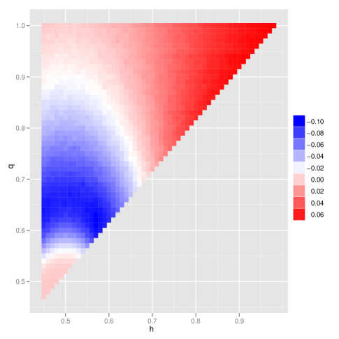
Figure 4: A comparison, using the limiting properties of $S_{1,0,0}(t;\Psi)$ and $S_{1,0,0}(t;\Phi)$, of $\beta_{\Psi}-\beta_{\Phi}$ for different null and alternative hypotheses pairs as parametrized by $h$ and $q(=p+\delta)$. The blue-colored region correspond to values of $h$ and $q(=p+\delta)$ for which $\beta_{\Psi}<\beta_{\Phi}$ while the red-colored region correspond to values of $h$ and $p+\delta$ with $\beta_{\Psi}>\beta_{\Phi}$.

We now analyze the use of Theorem 1 as a large-sample approximation to $S_{1,0,0}(t;\Phi)$ and $S_{1,0,0}(t;\Psi)$. From Figure 4 with $p=0.43$, we choose a $(h,p+\delta)$ pair, with $\beta_{\Psi}-\beta_{\Phi}>0.05$, namely $h=0.95$ and $p+\delta=0.98$. We then estimate the power of $\beta_{\Phi}$ and $\beta_{\Psi}$ by repeated sampling of graphs from stochastic blockmodel with parameters, $(\mathbf{P}^{0},n_{1},n_{2},n_{3})$ for the null distribution and $(\mathbf{P}^{A},n_{1},n_{2},n_{3})$ for the alternative distribution. The result is presented in Figure 5. We see that the large-sample approximation obtained via Theorem 1 matches well with sampling from the stochastic blockmodel (SBM). Figure 5 also includes power estimates for the random dot product model (RDPM) with varying concentration parameter $r$ and predetermined location parameters $\vec{\alpha}_{1},\vec{\alpha}_{2},\vec{\alpha}_{3}$. Specifically, $\vec{\alpha}_{1},\vec{\alpha}_{2},\vec{\alpha}_{3}$ are carefully chosen such that their Euclidean inner products match corresponding block connectivity probabilities i.e., $(p,h,q)$ specified above. We see that, as $r$ increases, the power estimates for the random dot product model matches well with those of the stochastic blockmodel and large-sample approximation. Finally Figure 5 also includes power estimates for the locality statistics based on $\Phi$ and $\Psi$ for $\tau=0$, i.e., no vertex-dependent normalization and is equivalent to the use of the max degree statistic to test $H_{0}$ against $H_{A}$. These are represented as dashed and dot blue lines, corresponding to large-sample approximation and Monte Carlo simulations, respectively. Clearly, vertex-dependent normalization leads to better performance for this $H_{0}$ and $H_{A}$ pair.

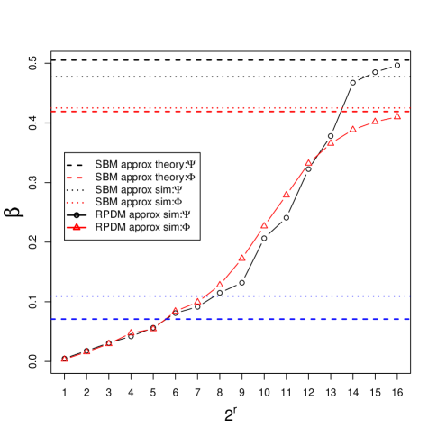
Figure 5: Power estimates $\beta_{\Psi}$ against $\beta_{\Phi}$ using Monte Carlo simulation on random graphs from the stochastic blockmodel, Monte Carlo simulation on random graphs from the random dot product model, and large-sample approximation for the stochastic blockmodel. $r$ is the concentration parameter. Dashed blue line: power estimate of large-sample approximation to $S_{0,0,0}(t;\Psi)$; dot blue line: power estimate of SBM Monte Carlo simulation to $S_{0,0,0}(t;\Psi)$.

VI Power Estimates of $S_{\tau=1,\ell=0,k=1}(t;\cdot)$

In this section, we provide investigations of $S_{\tau,\ell,k}(t;\Psi)$ and $S_{\tau,\ell,k}(t;\Phi)$ with a larger scale parameter $k=1$ instead of $k=0$. We keep $\tau=1$ and $\ell=0$ the same as before and derive the limiting properties of $\max_{v}(\Psi_{t;1}(v)-\Psi_{t-1;1}(v))$ and $\max_{v}(\Phi_{t,t;1}(v)-\Phi_{t,t-1;1}(v))$. To make conclusions concise and presentable, firstly, we delve into the limiting properties in the model presented in §  III with number of blocks $B=3$.

Proposition 3.

Assume the same setting in Theorem 1 with $B=3$. As $(n_{1},n_{2},n_{3})=(\Theta(n),o(n),o(n))$ and $n\to\infty$, $S_{1,0,1}(t;\Psi)$ has the following properties:

$$S_{1,0,1}(t;\Psi)=\max_{1\leq i\leq 3}W^{\prime}_{0}(n_{i};\Psi)\quad t<t^{\ast},$$

$$S_{1,0,1}(t;\Psi)=\max_{1\leq i\leq 3}W^{\prime}_{A}(n_{i};\Psi)\quad t=t^{\ast},$$

where

$$\dfrac{W^{\prime}_{0}({n_{i};\Psi)}-\mu^{\prime}_{0}(n_{i};\Psi)}{\gamma^{\prime}_{0}(n_{i};\Psi)}\stackrel{{\scriptstyle d}}{{\rightarrow}}\mathcal{G}(0,1)$$

$$\dfrac{W^{\prime}_{0}({n_{i};\Psi)}-\mu^{\prime}_{0}(n_{i};\Psi)}{\gamma^{\prime}_{0}(n_{i};\Psi)}\stackrel{{\scriptstyle d}}{{\rightarrow}}\mathcal{G}(0,1)$$

and the $\mu^{\prime}_{0},\mu^{\prime}_{A},\gamma^{\prime}_{0},\gamma^{\prime}_{A}$ are given by

$$\kappa^{\prime}(n,p,n_{2},h,i)=np^{2}+1+\bm{1}_{\{i=2\}}n_{2}p(h-p)$$

$$\mu^{\prime}_{0}(n_{i};\Psi)=\mu_{0}(n_{i};\Psi)\kappa^{\prime}(n,p,n_{2},h,i)$$

$$\gamma^{\prime}_{0}(n_{i};\Psi)=\gamma_{0}(n_{i};\Psi)\kappa^{\prime}(n,p,n_{2},h,i)$$

$$\begin{split}\zeta(n_{3},p,\delta,i)&=\dfrac{\delta}{2}[n_{3}^{2}(\bm{1}_{\{i\neq 3\}}p^{2}+\bm{1}_{\{i=3\}}(p+\delta)^{2})\\ +&n_{3}(\bm{1}_{\{i\neq 3\}}p(1-p)+\bm{1}_{\{i=3\}}(p+\delta)(1-p-\delta))]\end{split}$$

$$\begin{split}\mu^{\prime}_{A}(n_{i};\Psi)&=\mu_{A}(n_{i};\Psi)[\kappa^{\prime}(n,p,n_{2},h,i)+\frac{\bm{1}_{\{i=3\}}n_{3}p\delta}{2}]\\ &+\zeta(n_{3},p,\delta,i)\end{split}$$

$$\gamma^{\prime}_{A}(n_{i};\Psi) =\gamma_{A}(n_{i};\Psi)[\kappa^{\prime}(n,p,n_{2},h,i)+\frac{\bm{1}_{\{i=3\}}n_{3}p\delta}{2}].$$

Likewise,

$$S_{1,0,1}(t;\Phi)=\max_{1\leq i\leq 3}W^{\prime}_{0}(n_{i};\Phi)~{}t<t^{\ast},$$

$$S_{1,0,1}(t;\Phi)=\max_{1\leq i\leq 3}W^{\prime}_{A}(n_{i};\Phi)~{}t=t^{\ast},$$

where

$$\dfrac{W^{\prime}_{0}({n_{i};\Phi)}-\mu^{\prime}_{0}(n_{i};\Phi)}{\gamma^{\prime}_{0}(n_{i};\Phi)}\stackrel{{\scriptstyle d}}{{\rightarrow}}\mathcal{G}(0,1)$$

$$\dfrac{W^{\prime}_{0}({n_{i};\Phi)}-\mu^{\prime}_{0}(n_{i};\Phi)}{\gamma^{\prime}_{0}(n_{i};\Phi)}\stackrel{{\scriptstyle d}}{{\rightarrow}}\mathcal{G}(0,1)$$

and the $\mu^{\prime}_{0},\mu^{\prime}_{A},\gamma^{\prime}_{0},\gamma^{\prime}_{A}$ are given by

$$\eta(p)=p^{3}(1-p)$$

$$\xi_{0}(n_{i};\Phi)=\bm{1}_{\{i=2\}}n_{2}(h(1-h)-p(1-p))$$

$$\mu^{\prime}_{0}(n_{i};\Phi)=a_{n_{i}}\sqrt{Cn^{2}\eta(p)}+np(1-p)+\xi_{0}(n_{i};\Phi)$$

$$\gamma^{\prime}_{0}(n_{i};\Phi)=b_{n_{i}}\sqrt{Cn^{2}\eta(p)}$$

$$\begin{split}\zeta(n_{3},p,\delta,i)&=\dfrac{\delta}{2}[n_{3}^{2}(\bm{1}_{\{i\neq 3\}}p^{2}+\bm{1}_{\{i=3\}}(p+\delta)^{2})\\ &+n_{3}(\bm{1}_{\{i\neq 3\}}p(1-p)+\bm{1}_{\{i=3\}}(p+\delta)(1-p-\delta))]\end{split}$$

$$\mu^{\prime}_{A}(n_{i};\Phi) =\mu^{\prime}_{0}(n_{i};\Phi)+\bm{1}_{\{i=3\}}n_{3}\delta(1-p)+\zeta(n_{3},p,\delta,i)$$

$$\gamma^{\prime}_{A}(n_{i};\Phi) =\gamma^{\prime}_{0}(n_{i};\Phi)$$

Naturally, the limiting properties of $S_{1,0,1}(t;\Psi)$ and $S_{1,0,1}(t;\Phi)$ as given above offer the following power comparison result.

Proposition 4.

In the model shown in Figure1, Let $\alpha>0$ be given, $\beta^{\prime}_{\Phi}$ be the power of the test statistic $S_{1,0,1}(t;\Phi)$ when $t=t^{\ast}$ for testing the hypothesis that $t$ is change point at a significance level of $\alpha$ and $\beta^{\prime}_{\Psi}$ be the power of the test statistic $S_{1,0,1}(t;\Psi)$ when $t=t^{\ast}$ for testing the same hypothesis at the same significance level of $\alpha$. As $n\to\infty$, $\beta^{\prime}_{\Phi},\beta^{\prime}_{\Psi}$ and $\alpha$ have the following relationship:

1. $n_{3}=o(\sqrt{n})$ implies $\beta^{\prime}_{\Phi}=\beta^{\prime}_{\Psi}=\alpha$.

2. $n_{3}=\Omega(\sqrt{n})$ implies $\beta^{\prime}_{\Phi}\geq\beta^{\prime}_{\Psi}>\alpha$.

Consequently, Proposition 4 leads to the conclusion that the performance of $S_{1,0,1}(t;\Phi)$ dominates $S_{1,0,1}(t;\Psi)$ in the $3$-block model. Moreover, this superiority can be generalized to the case with any given number of blocks $B\geq 3$. This is because each block $[n_{i}]$ with $1<i<B$ in $B$-blocks model follows a similar probabilistic behavior as block $[n_{2}]$ in $3$-blocks model while the power of hypothesis testing is otherwise determined by the change of probabilistic behavior of block $[n_{B}]$. In the limiting condition with $n\to\infty$, both $\beta^{\prime}_{\Phi}$ and $\beta^{\prime}_{\Psi}$ in $B$-blocks model can be characterized as a function of $p,\delta,n_{B}$ only. In other words, though $h_{2}>p,\dots,h_{B-1}>p$, the ”chatty” groups $[n_{2}],\dots,[n_{B-1}]$ do not make any contribution on $\beta^{\prime}_{\Phi}$ or $\beta^{\prime}_{\Psi}$. Hence, the number of ”chatty groups”, namely $B-2$, is independent of the fact of dominance of $S_{1,0,1}(t;\Phi)$. Due to the superiority of $S_{1,0,1}(t;\Phi)$, only the limiting properties of $S_{1,0,1}(t;\Phi)$ in the general B-block model is given below.

Theorem 5.

Let $\{G_{t}\}$ be a time series of random graphs according to the alternative $H_{A}$ detailed in § III. In particular, $G_{t}\sim SBM(\mathbf{P}^{0},\{[n_{i}]_{i=1}^{B}\})$ for $t<t^{\ast}$ and $G_{t}\sim SBM(\mathbf{P}^{A},\{[n_{i}]_{i=1}^{B}\})$ for $t\geq t^{\ast}$ with $\mathbf{P}^{0}$ and $\mathbf{P}^{A}$ being of the form in Eq. (1) and Eq. (2), respectively. Let $S_{1,0,1}(t;\Phi)$ denote the statistic $S_{\tau,l,k}(t;\Phi)$ with $\tau=1$, $l=0$, and $k=1$.

Then as $n=\sum{n_{i}}\rightarrow\infty$, $S_{1,0,1}(t;\Phi)$ has the following properties:

$$S_{1,0,1}(t;\Phi)=\max_{1\leq i\leq B}W^{\prime}_{0}(n_{i};\Phi)\quad t<t^{\ast},$$

$$S_{1,0,1}(t;\Phi)=\max_{1\leq i\leq B}W^{\prime}_{A}(n_{i};\Phi)\quad t=t^{\ast},$$

where

$$\dfrac{W^{\prime}_{0}({n_{i};\Phi)}-\mu^{\prime}_{0}(n_{i};\Phi)}{\gamma^{\prime}_{0}(n_{i};\Phi)}\stackrel{{\scriptstyle d}}{{\rightarrow}}\mathcal{G}(0,1)$$

$$\dfrac{W^{\prime}_{A}({n_{i};\Phi)}-\mu^{\prime}_{A}(n_{i};\Phi)}{\gamma^{\prime}_{A}(n_{i};\Phi)}\stackrel{{\scriptstyle d}}{{\rightarrow}}\mathcal{G}(0,1)$$

and the $\mu^{\prime}_{0},\mu^{\prime}_{A},\gamma^{\prime}_{0},\gamma^{\prime}_{A}$ are given by

$$\eta(p)=p^{3}(1-p)$$

$$\xi_{0}(n_{i};\Phi)=\bm{1}_{\{i\notin\{1,B\}\}}n_{i}(h_{i}(1-h_{i})-p(1-p))$$

$$\mu^{\prime}_{0}(n_{i};\Phi)=a_{n_{i}}\sqrt{Cn^{2}\eta(p)}+np(1-p)+\xi_{0}(n_{i};\Phi)$$

$$\gamma^{\prime}_{0}(n_{i};\Phi)=b_{n_{i}}\sqrt{Cn^{2}\eta(p)}$$

$$\begin{split}\zeta(n_{B},p,\delta,i)&=\dfrac{\delta}{2}[n_{B}^{2}(\bm{1}_{\{i\neq B\}}p^{2}+\bm{1}_{\{i=B\}}(p+\delta)^{2})\\ +&n_{B}(\bm{1}_{\{i\neq B\}}p(1-p)+\bm{1}_{\{i=B\}}(p+\delta)(1-p-\delta))]\end{split}$$

$$\mu^{\prime}_{A}(n_{i};\Phi) =\mu^{\prime}_{0}(n_{i};\Phi)+\bm{1}_{\{i=B\}}n_{B}\delta(1-p)+\zeta(n_{B},p,\delta,i)$$

$$\gamma^{\prime}_{A}(n_{i};\Phi) =\gamma^{\prime}_{0}(n_{i};\Phi)$$

Corollary 6.

Assume the setting in Theorem 5. Let $\beta^{\prime}_{\Phi}$ be the power of the test statistic $S_{1,0,1}(t;\Phi)$ for $t=t^{\ast}$ and $\beta^{\prime}_{\Psi}$ be the power of the test statistic $S_{1,0,1}(t;\Psi)$ for $t=t^{\ast}$. Then, as $(n_{1},n_{2},\dots,n_{B})=(\Theta(n),o(n),\dots,o(n))$ and $n\to\infty$, $\beta^{\prime}_{\Phi}\geq\beta^{\prime}_{\Psi}$ and thus $S_{1,0,1}(t;\Psi)$ is inadmissible.

In §V and §VI, for simplicity of analytic investigations, we theoretically obtain power estimates of $S_{\tau,\ell,k}(t;\Psi)$ and $S_{\tau,\ell,k}(t;\Phi)$ under the restrictions of $\tau=1$ and $\ell=0$. Besides analytic investigations, we also empirically study power performances of $S_{\tau,\ell,k}(t;\Psi)$ and $S_{\tau,\ell,k}(t;\Phi)$ with other $(\tau,\ell)$ combinations via Monte Carlo simulations. In this experiment, we let $\tau$ range from $0$ to $10$ and $\ell$ range from $0$ to $10$. In each Monte Carlo replicate, a time series of random graphs based on the SBM considered in §V, where $(n_{1},n_{2},n_{3})=(870,65,65),(p,h,q)=(0.43,0.95,0.98)$, is sampled. Next, $S_{\tau,\ell,k}(t^{\ast}-1;\Psi)$,$S_{\tau,\ell,k}(t^{\ast}-1;\Phi)$,$S_{\tau,\ell,k}(t^{\ast};\Psi)$ and $S_{\tau,\ell,k}(t^{\ast};\Phi)$ are calculated individually according to specific $(\tau,\ell,k)$. After $2000$ replicates, for each test statistic, the largest empirical power (denoted by $\max_{(\tau,\ell)}\beta$) and the corresponding optimal choice of $(\tau,\ell)$ (denoted by $(\tau^{*},\ell^{*})$) is obtained and summarized in Table I.

TABLE I: The optimal $\tau$ and $l$ in an experiment comparing the statistical power of $S_{\tau,\ell,k}$ for $k=0,1$ and locality statistics $\Phi$ and $\Psi$. We varies $\tau,\ell\in\{0,1,\dots,10\}$ and compare the statistic power for each choice of $\tau$ and $\ell$ through a Monte-Carlo experiment with $2000$ replicates.

	$\max_{(\tau,\ell)}\beta$	$(\tau^{*},\ell^{*})$
$S_{\tau,\ell,0}(t;\Psi)$	$0.483$	$(1,0)$
$S_{\tau,\ell,0}(t;\Phi)$	$0.384$	$(1,10)$
$S_{\tau,\ell,1}(t;\Psi)$	0.571	(1,10)
$S_{\tau,\ell,1}(t;\Phi)$	0.758	(1,9)

The empirical results in Table I demonstrate the potential value of extending the theoretical investigations in §V and §VI to cases of $\tau\geq 1$ and $\ell\geq 1$, though this extension appears significantly more challenging than the case $(\tau,\ell)=(1,0)$.

VII Experiment

We use the Enron email data used in [19] for this experiment. It consists of time series of graphs $\{G_{t}\}$ with $|V|=184$ vertices for each week $t=1,\ldots,189$, where we draw a unweighted edge when vertex $v$ sends at least one email to vertex $w$ during a one week period.

After truncating first 40 weeks for vertex-standardized and temporal normalizations, Figure 6 depicts $S_{\tau,\ell,k}(t;\Psi)$ (SeaGreen) and $S_{\tau,\ell,k}(t;\Phi)$ (Orange) in the remaining 149 weeks from August 1999 to June 2002. In this experiment, we choose both $\tau=\ell=20$, used in [19], to keep the comparisons between the two papers meaningful. As indicated in [19], detections are defined as weeks $t$ such that $S_{\tau,\ell,k}>5$. Hence, from Figure 6 we have following observations and reasonings.

1. $S_{20,20,0}(t;\Psi),S_{20,20,0}(t;\Phi),S_{20,20,1}(t;\Psi),S_{20,20,1}(t;\Phi)$ and $S_{20,20,2}(t;\Phi)$ indicate a clear anomaly at $t^{*}=58$ in December 1999. This coincides with the happening of Enron’s tentative sham energy deal with Merrill Lynch to meet profit expectations and boost stock price [21]. The center of suspicious community-employee $v_{154}$ is identified by all five statistics.

2. $S_{20,20,0}(t;\Psi)$, $S_{20,20,0}(t;\Phi)$, $S_{20,20,1}(t;\Psi)$ and $S_{20,20,2}(t;\Psi)$ capture an anomaly at $t^{\ast}=146$ in the mid-August 2001. This is the period that Enron CEO Skilling made a resignation announcement when the company was surrounded by public criticisms shown in [21]. The center of suspicious community-employee $v_{95}$ is identified by these four statistics.

3. $S_{20,20,2}(t;\Psi)$ signifies an anomaly at $t^{\ast}=132$ in late April 2001 where $S_{20,20,k}(t;\Phi)$ fails to alert for any $k\in\{0,1,2\}$. This phenomenon occurs because $S_{20,20,2}(t;\Psi)$ captures the employee $v_{90}$ whose second-order neighborhood $N_{2}(v_{90};G_{132})$ contains $116$ emails at $t^{\ast}=132$ but $0$ email in his second-order neighborhoods of previous 20 weeks. That is, the time-dependent second-order neighborhood $N_{2}(v_{90};G_{t})$ had no communication in the period from $t=112$ to $t=131$. On the other hand, this behavior cannot be monitored by $S_{20,20,2}(132;\Phi)$ because the change of communication frequency in a fixed second-order neighborhood $N_{2}(v_{90};G_{132})$, measured by locality statistics $\Phi$, is not so significant. More concretely, the number of emails in the unchanged $N_{2}(v_{90};G_{132})$ has a mean of $45.5$ and a standard deviation of $14.9$ from $t=112$ to $t=131$. In [21], this anomaly appears after the Enron Quaterly Conference Call in which a Wall Street analyst Richard Grubman questioned Skilling on the company’s refusal of releasing balance sheet but then got insulted by Skilling.

4. $S_{20,20,2}(t;\Phi)$ shows a detection on $v_{135}$ at $t^{\ast}=136$ before June 2001 over $S_{20,20,2}(t;\Psi)$. This comes from the fact that the fixed second-order neighborhood of employee $v_{135}$ at $t^{\ast}=136$, i.e. $N_{2}(v_{135};G_{136})$, has a small standard deviation $1.08$ in previous 20 weeks while the communications in time-dependent neighborhoods $\{N_{2}(v_{90};G_{t})\}_{t=116}^{135}$ has a large standard deviation $10.04$. Practically speaking, in this case, a dramatic increment of email contacts in the certain community $N_{2}(v_{135};G_{136})$ could be captured by $S_{20,20,2}(t;\Phi)$ but ignored by $S_{20,20,2}(t;\Psi)$ because unstable communication patterns in $\{N_{2}(v_{90};G_{t})\}_{t=116}^{135}$ offsets the sensitivity of signal. According to [21], this anomaly corresponds to the formal notice of closure and termination of Enron’s single largest foreign investment, the Dabhol Power Company in India.

In summary, observations 1 and 2 demonstrate that in some cases both $S_{\tau,\ell,k}(t;\Psi)$ and $S_{\tau,\ell,k}(t;\Phi)$ are capable of capturing the same community which has a significant increment of connectivity. Besides, in some situations shown in observations 3 and 4, $S_{\tau,\ell,k}(t;\Psi)$ and $S_{\tau,\ell,k}(t;\Phi)$ achieve different detections due to its adaptability.

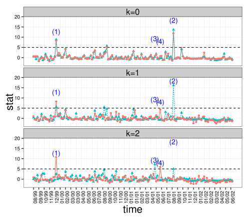
Figure 6: $S_{\tau,\ell,k}(t;\Psi)$(sea green) and $S_{\tau,\ell,k}(t;\Phi)$(orange), the temporally-normalized standardized scan statistics using $\tau=\ell=20$, in time series of Enron email-graphs from August 1999 to June 2002. Top: $k=0$; Middle: $k=1$; Bottom : $k=2$. In the case $k=0$, both $S_{20,20,0}(t;\Psi)$ and $S_{20,20,0}(t;\Phi)$ show detections ($S_{\tau,\ell,k}(t;\cdot)>5$) at observation mark (1) and (2); in the case $k=1$, both $S_{20,20,1}(t;\Psi)$ and $S_{20,20,1}(t;\Phi)$ show detections at observation mark (1), $S_{20,20,1}(t;\Psi)$ also indicates an anomaly at observation mark (2); in the case $k=2$, $S_{20,20,2}(t;\Psi)$ detects anomalies at observation mark (2) and (3) but $S_{20,20,2}(t;\Phi)$ captures anomalies at observation mark (1) and (4). Detailed analyses on each observation (1)(2)(3)(4) are provided in §VII respectively.

VIII Conclusion & Discussion

This paper has summarized a generative latent position model for time series of graphs and set up the change-point detection problem in time series of graphs in terms of stochastic block models. Then we have proposed the way of dealing with change-point detection through the use of scan statistics $S_{\tau,\ell,k}(t;\Psi)$ and $S_{\tau,\ell,k}(t;\Phi)$ constructed from two different locality statistics $\Psi$ and $\Phi$ respectively. We derived the limiting properties for four representative instances of locality-based scan statistics $S_{1,0,0}(t;\Psi),S_{1,0,0}(t;\Phi),S_{1,0,1}(t;\Psi)$ and $S_{1,0,1}(t;\Phi)$. The limiting properties were then used to derive estimates for the power of the tests.

The simulation experiments indicate that the analytic power estimates, even when they are limited in scope, are useful in answering some important questions about the locality statistics. In particular, it was shown that $\Psi$ and $\Phi$ are both admissible with respect to one another when $\tau=1,\ell=0,k=0$. In addition, if $\tau=1,\ell=0,k=1$, it is worthwhile to note that $\Psi$, compared with $\Phi$, is inadmissible but computationally inexpensive. For instance, in order to complete $\tau$-step vertex-dependent normalization calculation presented in Eq.(5), we have to record previous $\tau$-step graphs to calculate $J_{t,t^{\prime};k}(v)$ if the underlying locality statistic is $\Phi$. However, if the underlying locality statistic is $\Psi$, graph storage is not necessary and recording only the previous $\tau$-step statistics $\Psi_{t^{\prime};k}(v)$ is sufficient. Furthermore, the power estimates are also useful for reasoning about the behavior on more complicated models without $\{G_{t}\}$ independencies assumption, such as the latent process model proposed in [17]. [17] builds up a latent process model for time series of attributed graphs based on a random dot process model. Having $n$ vertices governed by $n$ individual continuous-time finite-state stochastic processes, this model generates a time series of dependent attributed random graphs, or equivalently, conditioning on the sample paths of the stochastic processes, the graphs are independent. [17] also provides two approximations to the exact latent process model. The first order approximation is the stochastic blockmodel which gives rise to a time series of independent random graphs with independent edges. The second order approximation corresponds to the random dot product model which gives rise to a time series of independent random dot product graphs. Both of these approximations are presented in § II.

The investigations presented in this paper do not take into account attributes on the edges. The incorporation of edge attributes into the current paper is, however, straightforward. For example, [22] handles attributes by linear fusion, and many of the results there can be adapted to the current paper. In particular, one can define fused locality statistics for attributed graphs. Power estimates for these locality statistics can be derived in a similar manner to those presented in this paper. Other considerations, e.g., optimal fusion parameters, can also be investigated. However, the statistics considered in [22] are only temporally normalized and does not contain a vertex dependent normalization. Thus, the derivation of their limiting properties are much less involved. In addition, as the experimental results in Fig 5 shown, the vertex dependent normalization does lead to improved statistical power in many situations of interest.

Anomaly detection in dynamic graphs has applications in diverse areas, e.g., predicting the emergence of subgroups within an organization, monitoring disease spread in public network, detecting modules of cancer and metastasis communities in Protein-protein interaction (PPI) network. We envision that these and many other applications will benefit from the kind of investigations outlined in this paper. However, much remains to be done, both mathematically and computationally. We list here some aspects that have not been (sufficiently) addressed in the paper.

1. Besides this paper, [22] also investigated $S_{\tau,\ell,k}(t;\Psi)$ for cases $\tau=0$, $\ell\to\infty$, and $k\leq 1$ under the SBM setting. However, power-estimates for other more complex locality-based scan statistics, such as $S_{\tau,\ell,k}(t;\cdot)$ for $1<\tau<\infty$, $0<\ell<\infty$ and $k\geq 2$, remain to be investigated.

2. Locality statistics based on $\Psi$ can be readily computed in a real-time streaming data environment, in contrast to those based on $\Phi$. Thus, the adaption or approximation of locality statistics based on $\Phi$ for streaming environments is of interest.

3. Power-estimates for locality statistics under the random dot product model setting. The limiting distributions, even for the simplest locality statistics, are currently unavailable.

Appendix A Appendix

In this appendix, we provide proofs of theorems, propositions and corollaries presented in § V and VI.

Theorem 1.

Firstly, we investigate the case that the underlying locality statistic is $\Psi$. We will derive the limiting property of $S_{1,0,0}(t;\Psi)$ for $t=t^{\ast}$ in some detail. The property of $S_{1,0,0}(t;\Psi)$ when $t<t^{\ast}$ can be derived in a similar manner.
As $\tau=1$ and $\ell=0$, for any $t$, we have $\widetilde{\Psi}_{t;1,0}(v)=\Psi_{t;0}(v)-\Psi_{t-1;0}(v)$ from Eq. (5) and Eq. (6). Without loss of generality, let us assume $v\in[n_{i}]$ and divide $\Psi_{t;0}(v)$ into two parts with $t=t^{\ast}$ and $t=t^{\ast}-1$:

$$\Psi_{t^{\ast};0}(v)=X_{1}+X_{2}$$

where $X_{1}\sim Bin(n-n_{i},p),X_{2}\sim Bin(n_{i}-1,\mathbf{P}^{A}_{i,i})$;

$$\Psi_{t^{\ast}-1;0}(v)=X_{3}+X_{4}$$

where $X_{3}\sim Bin(n-n_{i},p),X_{4}\sim Bin(n_{i}-1,\mathbf{P}^{0}_{i,i})$.
Since $G_{t^{\ast}-1}$ and $G_{t^{\ast}}$ are independent, we have

$$\begin{split}&\dfrac{\widetilde{\Psi}_{t^{\ast};1,0}(v)-(n_{i}-1)(\mathbf{P}^{A}_{i,i}-\mathbf{P}^{0}_{i,i})}{\sqrt{np(1-p)}}\\ =&\dfrac{\Psi_{t^{\ast};0}(v)-[(n-n_{i})p+(n_{i}-1)\mathbf{P}^{A}_{i,i}]}{\sqrt{np(1-p)}}\\ &-\dfrac{\Psi_{t^{\ast}-1;0}(v)-[(n-n_{i})p+(n_{i}-1)\mathbf{P}^{0}_{i,i}]}{\sqrt{np(1-p)}}\\ =&\dfrac{X_{1}-(n-n_{i})p}{\sqrt{(n-n_{i})p(1-p)}}\cdot\dfrac{\sqrt{(n-n_{i})p(1-p)}}{\sqrt{np(1-p)}}\\ &-\dfrac{X_{3}-(n-n_{i})p}{\sqrt{(n-n_{i})p(1-p)}}\cdot\dfrac{\sqrt{(n-n_{i})p(1-p)}}{\sqrt{np(1-p)}}\\ &+\dfrac{X_{2}-(n_{i}-1)\mathbf{P}^{A}_{i,i}}{\sqrt{(n_{i}-1)\mathbf{P}^{A}_{i,i}(1-\mathbf{P}^{A}_{i,i})}}\cdot\dfrac{\sqrt{(n_{i}-1)\mathbf{P}^{A}_{i,i}(1-\mathbf{P}^{A}_{i,i})}}{\sqrt{np(1-p)}}\\ &-\dfrac{X_{4}-(n_{i}-1)\mathbf{P}^{0}_{i,i}}{\sqrt{(n_{i}-1)\mathbf{P}^{0}_{i,i}(1-\mathbf{P}^{0}_{i,i})}}\cdot\dfrac{\sqrt{(n_{i}-1)\mathbf{P}^{0}_{i,i}(1-\mathbf{P}^{0}_{i,i})}}{\sqrt{np(1-p)}}\\ \xrightarrow{d}&~{}\mathcal{N}(0,1)\cdot C_{1}-\mathcal{N}(0,1)\cdot C_{2}+\mathcal{N}(0,1)\cdot C_{3}-\mathcal{N}(0,1)\cdot C_{4}\\ \xrightarrow{d}&~{}\mathcal{N}(0,C)\\ \end{split}$$ (18)

where

$$C_{1} =C_{2}=\lim_{n\to\infty}\sqrt{\dfrac{n-n_{i}}{n}},$$

$$C_{3} =\dfrac{\sqrt{(n_{i}-1)\mathbf{P}^{A}_{i,i}(1-\mathbf{P}^{A}_{i,i})}}{\sqrt{np(1-p)}},$$

$$C_{4} =\dfrac{\sqrt{(n_{i}-1)\mathbf{P}^{0}_{i,i}(1-\mathbf{P}^{0}_{i,i})}}{\sqrt{np(1-p)}},$$

$$C =\sum_{i=1}^{i=4}C_{i}^{2}$$

Next, plug in $\mathbf{P}^{A}_{i,i}$ and $\mathbf{P}^{0}_{i,i}$ into Eq. (18), we obtain

$$\dfrac{\widetilde{\Psi}_{t^{\ast};1,0}(v)-\mathbf{1}_{\{i=B\}}n_{B}\delta}{\sqrt{Cnp(1-p)}}\xrightarrow{d}\mathcal{N}(0,1),~{}v\in[n_{i}]$$

We can show that the dependency among the $\{\widetilde{\Psi}_{t^{\ast};1,0}(v)\}_{v\in V(G_{t})}$ is negligible by showing that the correlation between any two of the $\widetilde{\Psi}_{t^{\ast};1,0}(v)$ goes to $0$ sufficiently fast as $n\rightarrow\infty$. For $u$ and $v$ in block $[n_{i}]$,

$$corr(\widetilde{\Psi}_{t^{\ast};1,0}(u),\widetilde{\Psi}_{t^{\ast};1,0}(v))\leq\dfrac{1}{Cnp(1-p)}=O(\dfrac{1}{n})$$

Hence, the sample maximum of $\{Y_{v}\}_{v\in[n_{i}]}$ converges to the sample maximum of $n_{i}$ i.i.d $\mathcal{N}(0,1)$ random variables where $Y_{v}=\dfrac{\widetilde{\Psi}_{t^{\ast};1,0}(v)-\mathbf{1}_{\{i=B\}}n_{B}\delta}{\sqrt{Cnp(1-p)}}$ ([23], Theorem $3.1$). Also, it is known that the sample maximum of i.i.d $\mathcal{N}(0,1)$ random variables weakly converges to the Gumbel distribution ([24], § $2.3$). One then verifies that the composition of above weak convergences still holds (see e.g. proof of Proposition 5 in [22]) and we thus have

$$\dfrac{W_{A}(n_{i};\Psi)-\mu_{A}(n_{i};\Psi)}{\gamma_{A}(n_{i};\Psi)}\stackrel{{\scriptstyle d}}{{\rightarrow}}\mathcal{G}(0,1).$$

Eq.(8) and Eq. (9) then implies that

$$S_{1,0,0}(t^{\ast};\Psi)=\max_{v\in[n]}\widetilde{\Psi}_{t^{\ast};1,0}(v)=\max_{1\leq i\leq B}\{W_{A}(n_{i};\Psi)\}.$$

That is, the maximum of $\widetilde{\Psi}_{t^{\ast};1,0}(v)$ over all $n$ vertices is equivalent to the maximum of $W_{A}(n_{i};\Psi)$ over all $B$ blocks where $W_{A}(n_{i};\Psi)$ converges to $\mathcal{G}(0,1)$ under proper normalization

Similarly, the case when $t<t^{\ast}$ can be derived through the same approaches above. The limiting property of $S_{1,0,0}(t;\Psi)$ with $t<t^{\ast}$ then has the form in Eq. (14) with variations of $\mu_{0}(n_{i};\Psi)$ and $\gamma_{0}(n_{i};\Psi)$ for the normalization of $W_{0}(n_{i};\Psi)$.

We now consider the case where the underlying locality statistic being $\Phi$. The derivation of limiting property of $S_{1,0,0}(t;\Phi)$ for $t=t^{\ast}$ is given below. The derivation of the limiting property of $S_{1,0,0}(t;\Phi)$ for $t<t^{\ast}$ is similar and can be obtained with minor changes.
Let’s assume $v\in[n_{i}]$, from Eq.(4) to (6),

$$\Phi_{t^{\ast},t^{\ast};0}(v)=X_{1}+X_{2}$$

where $X_{1}\sim Bin(n-n_{i},p),X_{2}\sim Bin(n_{i}-1,\mathbf{P}^{A}_{i,i})$ and

$$\Phi_{t^{\ast},t^{\ast}-1;0}(v)|G_{t^{\ast}}=X_{3}+X_{4}$$

where $X_{3}\sim Bin(X_{1},p),X_{4}\sim Bin(X_{2},\mathbf{P}^{0}_{i,i})$.

Because $\widetilde{\Phi}_{t^{\ast};1,0}(v)=\Phi_{t^{\ast},t^{\ast};0}(v)-\Phi_{t^{\ast},t^{\ast}-1;0}(v)$, $\widetilde{\Phi}_{t^{\ast};1,0}(v)$ counts the number of edges, for vertex $v$, appearing in $G_{t^{\ast}}$ but disappearing in $G_{t^{\ast}-1}$. Accordingly, the edge is independently counted with probability $\mathbf{P}^{A}_{i,i}(1-\mathbf{P}^{0}_{i,i})$ to neighbors in $[n_{i}]$ and $p(1-p)$ to neighbors in $[n]\backslash[n_{i}]$ respectively. That is,

$$\widetilde{\Phi}_{t^{\ast};1,0}(v)=B_{3}+B_{4}$$

where $B_{3}\sim Bin(n-n_{i},p(1-p)),B_{4}\sim Bin(n_{i}-1,\mathbf{P}^{A}_{i,i}(1-\mathbf{P}^{0}_{i,i}))$.

By the central limit theorem, we have

$$\begin{split}&\dfrac{\widetilde{\Phi}_{t^{\ast};1,0}(v)-[(n-n_{i})p(1-p)+(n_{i}-1)\mathbf{P}^{A}_{i,i}(1-\mathbf{P}^{0}_{i,i})]}{\sqrt{np(1-p)[1-p(1-p)]}}\\ =&\dfrac{B_{3}-(n-n_{i})p(1-p)}{\sqrt{(n-n_{i})p(1-p)[1-p(1-p)]}}\\ &\cdot\dfrac{\sqrt{(n-n_{i})p(1-p)[1-p(1-p)]}}{\sqrt{np(1-p)[1-p(1-p)]}}\\ &+\\ &\dfrac{B_{4}-(n_{i}-1)\mathbf{P}^{A}_{i,i}(1-\mathbf{P}^{0}_{i,i})}{\sqrt{(n_{i}-1)\mathbf{P}^{A}_{i,i}(1-\mathbf{P}^{0}_{i,i})[1-\mathbf{P}^{A}_{i,i}(1-\mathbf{P}^{0}_{i,i})]}}\\ \cdot&\dfrac{\sqrt{(n_{i}-1)\mathbf{P}^{A}_{i,i}(1-\mathbf{P}^{0}_{i,i})[1-\mathbf{P}^{A}_{i,i}(1-\mathbf{P}^{0}_{i,i})]}}{\sqrt{np(1-p)[1-p(1-p)]}}\\ \xrightarrow{d}&\mathcal{N}(0,1)\cdot C_{1}+\mathcal{N}(0,1)\cdot C_{2}\\ \xrightarrow{d}&~{}\mathcal{N}(0,C)\\ \end{split}$$ (19)

where

$$C_{1} =\lim_{n\to\infty}\sqrt{\dfrac{n-n_{i}}{n}},$$

$$C_{2} =\lim_{n\to\infty}\dfrac{\sqrt{(n_{i}-1)\mathbf{P}^{A}_{i,i}(1-\mathbf{P}^{0}_{i,i})[1-\mathbf{P}^{A}_{i,i}(1-\mathbf{P}^{0}_{i,i})]}}{\sqrt{np(1-p)[1-p(1-p)]}},$$

$$C =\sum_{i=1}^{i=2}C_{i}^{2}.$$

Similarly, after plugging $\mathbf{P}^{0}_{i,i}$ and $\mathbf{P}^{A}_{i,i}$ into Eq. (19), we obtain

$$\begin{split}&\dfrac{\widetilde{\Phi}_{t^{\ast};1,0}(v)-np(1-p)-\xi_{0}(n_{i};\Phi)-\mathbf{1}_{\{i=B\}}n_{B}\delta(1-p)}{\sqrt{Cnp(1-p)[1-p(1-p)]}}\\ \xrightarrow{d}&\mathcal{N}(0,1).\end{split}$$

For locality statistic $\Phi$, the dependency among $\{\widetilde{\Phi}_{t^{\ast};1,0}(v)\}_{v\in[n]}$ is also negligible because

$$\begin{split}&corr(\widetilde{\Phi}_{t^{\ast};1,0}(u),\widetilde{\Phi}_{t^{\ast};1,0}(v))\\ =&\dfrac{cov(\widetilde{\Phi}_{t^{\ast};1,0}(u),\widetilde{\Phi}_{t^{\ast};1,0}(v))}{{Cnp(1-p)[1-p(1-p)]}}\\ \leq&\dfrac{1}{Cn{p(1-p)[1-p(1-p)]}}=O(\dfrac{1}{n})\end{split}$$

Therefore by following the same procedures of reasoning the limiting distribution of $W_{A}(n_{i};\Psi)$, we can also obtain

$$\dfrac{W_{A}(n_{i};\Phi)-\mu_{A}(n_{i};\Phi)}{\gamma_{A}(n_{i};\Phi)}\stackrel{{\scriptstyle d}}{{\rightarrow}}\mathcal{G}(0,1)$$

where $W_{A}(n_{i};\Phi)=\max_{v\in[n_{i}]}\widetilde{\Phi}_{t^{\ast};1,0}(v)$.
Thus, $S_{1,0,0}(t^{\ast};\Phi)$ is the maximum of $W_{A}(n_{i};\Phi)$ over $B$ blocks as desired. ∎

Corollary 2.

The limiting distributions of $\widetilde{\Psi}_{t^{\ast}-1;1,0}(v)$ and $\widetilde{\Psi}_{t^{\ast};1,0}(v)$ derived in the proof Theorem 1 provides that, under $H_{0}$,

$$\dfrac{\widetilde{\Psi}_{t^{\ast}-1;1,0}(v)-0}{\sqrt{Cnp(1-p)}}\xrightarrow{d}\mathcal{N}(0,1),~{}v\in[n_{i}]$$

and, under $H_{A}$,

$$\dfrac{\widetilde{\Psi}_{t^{\ast};1,0}(v)-\mathbf{1}_{\{i=3\}}n_{3}\delta}{\sqrt{Cnp(1-p)}}\xrightarrow{d}\mathcal{N}(0,1),~{}v\in[n_{i}]$$

Accordingly, the ratio of the shift in the mean, from null to alternative, over the standard deviation of $\widetilde{\Psi}_{t;1,0}(v)$ for each vertex would be $\dfrac{\mathbf{1}_{\{i=3\}}n_{3}\delta}{\sqrt{Cnp(1-p)}}$. We obtain two relationships between $\beta_{\Psi}$ and $\alpha$ on the basis of the order of $n_{3}$:

1. if $n_{3}=o(\sqrt{n})$, the ratio approaches to $0$ and thus implies $\beta_{\Psi}=\alpha$.

2. if $n_{3}=\Omega(\sqrt{n})$, then $\exists k>0$ such that $\dfrac{\mathbf{1}_{\{i=3\}}n_{3}\delta}{\sqrt{Cnp(1-p)}}\geq k>0$ as $n\to\infty$ which implies $\beta_{\Psi}>\alpha$.

Likewise, from Theorem 1, the limiting distributions of $\widetilde{\Phi}_{t;1,0}(v)$ under null and alternative respectively are

$$\begin{split}&\dfrac{\widetilde{\Phi}_{t^{\ast}-1;1,0}(v)-np(1-p)-\xi_{0}(n_{i};\Phi)}{\sqrt{Cnp(1-p)[1-p(1-p)]}}\xrightarrow{d}\mathcal{N}(0,1).\end{split}$$

$$\begin{split}&\dfrac{\widetilde{\Phi}_{t^{\ast};1,0}(v)-np(1-p)-\xi_{0}(n_{i};\Phi)-\mathbf{1}_{\{i=3\}}n_{3}\delta(1-p)}{\sqrt{Cnp(1-p)[1-p(1-p)]}}\\ \xrightarrow{d}&\mathcal{N}(0,1).\end{split}$$

The relationship between $\beta_{\Phi}$ and $\alpha$ is more involved when $\xi_{0}(n_{2};\Phi)$ are included. In order to clarify the order dominance relationship between $\xi_{0}(n_{2};\Phi)$ and $n_{3}\delta(1-p)$, there are five separate cases to be considered:

1. if $n_{3}=o(\sqrt{n})$, as $n\to\infty$, $\widetilde{\Phi}_{t;1,0}(v)$ share the same mean and variance under both $H_{0}$ and $H_{A}$, thus $\beta_{\Phi}=\alpha$.

2. if $n_{3}=\Theta{(\sqrt{n})}=\Theta(n_{2})$, $\dfrac{n_{3}\delta(1-p)}{\sqrt{Cnp(1-p)[1-p(1-p)]}}$ and $\dfrac{\xi_{0}(n_{2};\Phi)}{\sqrt{Cnp(1-p)[1-p(1-p)]}}$ have the same order $\Theta(1)$ so that the increment ,$\dfrac{n_{3}\delta(1-p)}{\sqrt{Cnp(1-p)[1-p(1-p)]}}=\Theta(1)$, is not negligible and implies $\beta_{\Phi}>\alpha$.

3. if $n_{3}=\omega{(\sqrt{n})}=\Theta{(n_{2})}$, whether $\beta_{\Phi}>\alpha$ is determined by if $P(\operatornamewithlimits{argmax}\widetilde{\Phi}_{t;1,0}(v)\in[n_{3}])$ under $H_{A}$ is larger than under $H_{0}$. In fact, if $\dfrac{\xi_{0}(n_{2};\Phi)}{n_{3}\delta(1-p)}>1$, $P(\operatornamewithlimits{argmax}\widetilde{\Phi}_{t;1,0}(v)\in[n_{2}])=1$ as $n\to\infty$ under both $H_{0}$ and $H_{A}$, hence $\beta_{\Phi}=\alpha$. Otherwise, $n_{3}\delta(1-p)$ in $[n_{3}]$ contributes to the power increment.

4. if $n_{3}=\Omega{(\sqrt{n})}=\omega(n_{2})$, $n_{3}\delta(1-p)$ dominates $\xi_{0}(n_{2};\Phi)$ in the limit thereby the location shift in block $[n_{3}]$ results in $P(\operatornamewithlimits{argmax}\widetilde{\Phi}_{t^{\ast};1,0}(v)\in[n_{3}])=1$ and thus $\beta_{\Phi}>\alpha$.

5. if $n_{3}=\Omega{(\sqrt{n})}=o{(n_{2})}$, whether $n_{3}\delta(1-p)$ leads to a power increment depends on the sign of $\xi_{0}(n_{2};\Phi)$. If $h+p<1$ such that $\xi_{0}(n_{2};\Phi)$ being positive, $P(\operatornamewithlimits{argmax}\widetilde{\Phi}_{t;1,0}(v)\in[n_{2}])=1$ under both $H_{0}$ and $H_{A}$ as $n\to\infty$ because $n_{3}=o(n_{2})$. On the contrary, if $h+p\geq 1$, $\xi_{0}(n_{2};\Phi)<0$ enables $P(\operatornamewithlimits{argmax}\widetilde{\Phi}_{t;1,0}(v)\in[n_{3}])$ to increase from $H_{0}$ to $H_{A}$. Thus, we have $\beta_{\Phi}=\alpha\,\,\text{if $h+p<1$};\beta_{\Phi}>\alpha\,\,\text{if $h+p\geq 1$}.$

∎

Proposition 3.

We present a sketch of the proof based on arguments from [25] for the case where the underlying locality statistic is $\Psi$. The case where the underlying locality statistic is $\Phi$ follows from the proof of Theorem 5.

Let $v\in[n_{i}](i\in\{1,2,3\})$, locality statistics $\Psi_{t^{\ast},t^{\ast};1}(v)$ and $\Psi_{t^{\ast},t^{\ast}-1;1}(v)$ are respectively decomposed as follows

$$\Psi_{t^{\ast},t^{\ast};1}(v)=X_{i}+\sum_{j\neq i}X_{j}+\sum_{j=1}^{3}Y_{j}+\sum_{1\leq j<k\leq 3}^{3}Z_{jk},~{}v\in[n_{i}]$$

where

$$X_{i} \sim Bin(n_{i}-1,\mathbf{P}^{A}_{i,i}),$$

$$X_{j} \sim Bin(n_{j},\mathbf{P}^{A}_{i,j}),$$

$$Y_{j}|X_{j} \sim Bin({X_{j}\choose 2},\mathbf{P}^{A}_{j,j}),$$

$$Z_{jk}|X_{j},X_{k} \sim Bin(X_{j}X_{k},\mathbf{P}^{A}_{j,k}).$$

and

$$\Psi_{t^{\ast},t^{\ast}-1;1}(v)=X^{\prime}_{i}+\sum_{j\neq i}X^{\prime}_{j}+\sum_{j=1}^{3}Y^{\prime}_{j}+\sum_{1\leq j<k\leq 3}^{3}Z^{\prime}_{jk},~{}v\in[n_{i}]$$

where

$$X^{\prime}_{i} \sim Bin(n_{i}-1,\mathbf{P}^{0}_{i,i}),$$

$$X^{\prime}_{j} \sim Bin(n_{j},\mathbf{P}^{0}_{i,j}),$$

$$Y^{\prime}_{j}|X^{\prime}_{j} \sim Bin({X^{\prime}_{j}\choose 2},\mathbf{P}^{0}_{j,j}),$$

$$Z^{\prime}_{jk}|X^{\prime}_{j},X^{\prime}_{k} \sim Bin(X^{\prime}_{j}X^{\prime}_{k},\mathbf{P}^{0}_{j,k}).$$

Hence, when $\mathbf{P}^{0}$ and $\mathbf{P}^{A}$ are substituted, we have

$$\widetilde{\Psi}_{t^{\ast};1,1}(v)=\Psi_{t^{\ast},t^{\ast};1}(v)-\Psi_{t^{\ast},t^{\ast}-1;1}(v)$$

$$\begin{split}=&[(X_{i}+\sum_{j\neq i}X_{j})-(X^{\prime}_{i}+\sum_{j\neq i}X^{\prime}_{j})]\\ &+[(\sum_{j=1}^{3}Y_{j}+\sum_{1\leq j<k\leq 3}^{3}Z_{jk})-(\sum_{j=1}^{3}Y^{\prime}_{j}+\sum_{1\leq j<k\leq 3}^{3}Z^{\prime}_{jk})]\\ =&[(X_{i}+\sum_{j\neq i}X_{j})-(X^{\prime}_{i}+\sum_{j\neq i}X^{\prime}_{j})]\cdot\\ &\Big{[}1+\dfrac{p}{2}[(X^{\prime}_{i}+\sum_{j\neq i}X^{\prime}_{j})+(X_{i}+\sum_{j\neq i}X_{j})]\Big{]}\\ &+\dfrac{h-p}{2}(X_{2}^{2}-{X^{\prime}_{2}}^{2})+\dfrac{\delta}{2}X^{2}_{3}\\ =&\widetilde{\Psi}_{t^{\ast};1,0}(v)\cdot\Big{[}1+\dfrac{p}{2}[(X^{\prime}_{i}+\sum_{j\neq i}X^{\prime}_{j})+(X_{i}+\sum_{j\neq i}X_{j})]\Big{]}\\ &+\dfrac{h-p}{2}(X_{2}^{2}-{X^{\prime}_{2}}^{2})+\dfrac{\delta}{2}X^{2}_{3}\end{split}$$

Thus, by using similar approaches given in the proof of lemma $3.2$ and lemma $3.3$ from [25], we obtain, as $n\to\infty$,

$$\arg max_{v\in[n_{i}]}\widetilde{\Psi}_{t^{\ast};1,0}(v)=\arg max_{v\in[n_{i}]}\widetilde{\Psi}_{t^{\ast};1,1}(v)$$

and

$$\begin{split}&\lim P(W^{\prime}_{A}(n_{i};\Psi)>\mu^{\prime}_{A}(n_{i};\Psi))\\ =&\lim P(W_{A}(n_{i};\Psi)>\mu_{A}(n_{i};\Psi))\end{split}$$

where $W^{\prime}_{A}(n_{i};\Psi)=\max_{v\in[n_{i}]}\widetilde{\Psi}_{t^{\ast};1,1}(v)$ and $W_{A}(n_{i};\Psi)=\max_{v\in[n_{i}]}\widetilde{\Psi}_{t^{\ast};1,0}(v)$. This leads to the fact that $(W^{\prime}_{A}(n_{i};\Psi)-\mu^{\prime}_{A}(n_{i};\Psi))/\beta^{\prime}_{A}(n_{i};\Psi)$ follows standard Gumbel distribution $\mathcal{G}(0,1)$ and $S_{1,0,1}(t^{\ast};\Phi)=\max_{1\leq i\leq 3}W^{\prime}_{A}(n_{i};\Phi)$. Similar arguments apply to $S_{1,0,1}(t^{\ast}-1;\Psi)$. ∎

Before proving Theorem 5, we state and prove a technical lemma on the correlations among the $\{\widetilde{\Phi}_{t;1,1}(v)\}$.

Lemma 7.

Let $G_{t-1}$ and $G_{t}$ be two independent Erdös-Rényi graphs with connectivity probability $p$, i.e., $G_{t-1}\sim G(n,p)$ and $G_{t}\sim G(n,p)$. For each $v$, $\widetilde{\Phi}_{t;1,1}(v)$ is defined according to Eq. (5). Then for any pair of vertices $u$ and $v$, the correlation between $\widetilde{\Phi}_{t;1,1}(u)$ and $\widetilde{\Phi}_{t;1,1}(v)$ is of order $O(\tfrac{1}{n})$ for $n\rightarrow\infty$.

Proof.

From Eq. (5) and (6), for any pair of vertices $(u,v)$,

$$\begin{split}&cov(\widetilde{\Phi}_{t;1,1}(u),\widetilde{\Phi}_{t;1,1}(v))\\ =&cov({\Phi}_{t,t;1}(u),{\Phi}_{t,t;1}(v))-cov({\Phi}_{t,t;1}(u),{\Phi}_{t,t-1;1}(v))-\\ &cov({\Phi}_{t,t-1;1}(u),{\Phi}_{t,t;1}(v))+cov({\Phi}_{t,t-1;1}(u),{\Phi}_{t,t-1;1}(v))\end{split}$$ (20)

We then consider to decompose ${\Phi}_{t,t;1}(u)$ into two parts representing the cardinalities of two disjoint sets of edges.

$$\begin{split}{\Phi}_{t,t;1}(u)=X_{t}(u)+Y_{t}(u)\end{split}$$

where the intuitive interpretations behind two terms are listed below:

$$X_{t}(u)= |\{(u,w):(u,w)\in E(G_{t})\text{ and }w\in N_{1}(u;G_{t})\backslash\{u\}\}|$$

$$Y_{t}(u)= |\{(w_{1},w_{2}):(w_{1},w_{2})\in E(G_{t}),w_{1}<w_{2}\text{ and }$$

$$w_{1},w_{2}\in N_{1}(u;G_{t})\backslash\{u\}\}|$$

Also, ${\Phi}_{t,t-1;1}(u)$ is decomposed into two terms as well.

$$\begin{split}{\Phi}_{t,t-1;1}(u)=X_{t-1}(u)+Y_{t-1}(u)\end{split}$$

where the intuitive interpretations behind two terms are listed below:

$$X_{t-1}(u)= |\{(u,w):(u,w)\in E(G_{t})\cap E(G_{t-1})$$

$$\text{ and }w\in N_{1}(u;G_{t})\backslash\{u\}|$$

$$Y_{t-1}(u)= |\{(w_{1},w_{2}):(w_{1},w_{2})\in E(G_{t-1}),w_{1}<w_{2}\text{ and }$$

$$w_{1},w_{2}\in N_{1}(u;G_{t})\backslash\{u\}\}|$$

Similarly, ${\Phi}_{t,t;1}(v)$ and ${\Phi}_{t,t-1;1}(v)$ are decomposed with the same structure. By expanding above decompositions into Eq. (20), we have the following table recording $16$ terms and their signs in (20).

TABLE II: Decomposition of the covariance terms in $S_{\tau,l,k}(\cdot,\Psi)$ for $\tau=1,l=0,k=1$.

$cov(\cdot,\cdot)$	$X_{t}(v)$	$X_{t-1}(v)$	$Y_{t}(v)$	$Y_{t-1}(v)$
$X_{t}(u)$	$+$	$-$	$\color[rgb]{0,0,1}+$	$\color[rgb]{0,0,1}-$
$X_{t-1}(u)$	$-$	$+$	$\color[rgb]{0,1,0}-$	$\color[rgb]{0,1,0}+$
$Y_{t}(u)$	$\color[rgb]{0,0,1}+^{\dagger}$	$\color[rgb]{0,1,0}-^{\ddagger}$	$\color[rgb]{1,0,1}+^{\amalg}$	$\color[rgb]{1,0,1}-$
$Y_{t-1}(u)$	$\color[rgb]{0,0,1}-^{\dagger}$	$\color[rgb]{0,1,0}+^{\ddagger}$	$\color[rgb]{1,0,1}-^{\amalg}$	$\color[rgb]{1,0,1}+$

In Table II, all terms earning the same color (blue, green or magenta) and same positive/negative sign are symmetric. Additionally, the terms having the same mark ($\dagger,\ddagger$ or $\amalg$) are canceled out due to the fact $Y_{t}(\cdot)|X_{t}(\cdot)\stackrel{{\scriptstyle iid}}{{\sim}}Y_{t-1}(\cdot)|X_{t}(\cdot)$. More concretely, for example, for four terms marked by blue, we have $cov(X_{t}(u),Y_{t}(v))=cov(Y_{t}(u),X_{t}(v))=cov(Y_{t-1}(u),X_{t}(v))=cov(X_{t}(u),Y_{t-1}(v))$. The first and third equality are guaranteed by symmetry property. The second equality holds because $Y_{t}(u)$ and $Y_{t-1}(u)$ share the same conditional distribution, $Bin({X_{t}(u)\choose 2},p)$, given $X_{t}(u)$. That is, $cov(Y_{t}(u),X_{t}(v)|X_{t}(u))=cov(Y_{t-1}(u),X_{t}(v)|X_{t}(u))$ and hence $cov(Y_{t}(u),X_{t}(v))=cov(Y_{t-1}(u),X_{t}(v))$ with application of law of total covariance.
We now return to Eq. (20). The above reasoning gives

$$\begin{split}&cov(\widetilde{\Phi}_{t;1,1}(u),\widetilde{\Phi}_{t;1,1}(v))\\ =&cov(X_{t}(u),X_{t}(v))-cov(X_{t}(u),X_{t-1}(v))-\\ &cov(X_{t-1}(u),X_{t}(v))+cov(X_{t-1}(u),X_{t-1}(v))\\ =&O(n).\end{split}$$

The last equality holds because the Cauchy-Schwarz inequality guarantees each of fours term are $O(n)$ where $X_{t}(\cdot)\sim Bin(n-1,p)$ and $X_{t-1}(\cdot)\sim Bin(n-1,p^{2})$.

In the following, to compute $var(\widetilde{\Phi}_{t;1,1}(u))$, $\widetilde{\Phi}_{t;1,1}(u)$ is decomposed as

$$\widetilde{\Phi}_{t;1,1}(u)=X_{t}+Y_{t}-X_{t-1}-Y_{t-1}$$

where

$$X_{t} \sim Bin(n-1,p),$$

$$Y_{t}|X_{t} \sim Bin({X_{t}\choose 2},p),$$

$$X_{t-1}|X_{t} \sim Bin(X_{t},p),$$

$$Y_{t-1}|X_{t} \sim Bin({X_{t}\choose 2},p),$$

$$Y_{t}|X_{t} \perp Y_{t-1}|X_{t}.$$

By applying law of total variance, we reach the following variance order estimation

$$\begin{split}&var(\widetilde{\Phi}_{t;1,1}(u))\\ =&\Theta(var(Y_{t}-Y_{t-1}))\\ =&\Theta(E[var(Y_{t}-Y_{t-1}|X_{t})]+var[E(Y_{t}-Y_{t-1}|X_{t})])\\ =&\Theta(E[2{X_{t}\choose 2}p(1-p)]+var[0])\\ =&\Theta(n^{2}p^{3}(1-p))\end{split}$$

Therefore, it follows that

$$corr(\widetilde{\Phi}_{t;1,1}(u),\widetilde{\Phi}_{t;1,1}(v))=O(\dfrac{1}{n})$$

as desired. ∎

Theorem 5.

Again, to avoid redundant arguments, we only provide derivations of limiting distribution of $\widetilde{\Phi}_{t^{\ast};1,1}(v)$ and the case $t<t^{\ast}$ can be achieved in the same approach. Let $v\in[n_{i}]$, locality statistics $\Phi_{t^{\ast},t^{\ast};1}(v)$ and $\Phi_{t^{\ast},t^{\ast}-1;1}(v)$ are respectively decomposed as follows:

$$\Phi_{t^{\ast},t^{\ast};1}(v)=X_{i}+\sum_{j\neq i}X_{j}+\sum_{j=1}^{B}Y_{j}+\sum_{1\leq j<k\leq B}^{B}Z_{jk},~{}v\in[n_{i}]$$ (21)

where

$$X_{i} \sim Bin(n_{i}-1,\mathbf{P}^{A}_{i,i}),$$

$$X_{j} \sim Bin(n_{j},\mathbf{P}^{A}_{i,j}),$$

$$Y_{j}|X_{j} \sim Bin({X_{j}\choose 2},\mathbf{P}^{A}_{j,j}),$$

$$Z_{jk}|X_{j},X_{k} \sim Bin(X_{j}X_{k},\mathbf{P}^{A}_{j,k}).$$

and

$$\Phi_{t^{\ast},t^{\ast}-1;1}(v)=X^{\prime}_{i}+\sum_{j\neq i}X^{\prime}_{j}+\sum_{j=1}^{B}Y^{\prime}_{j}+\sum_{1\leq j<k\leq B}^{B}Z^{\prime}_{jk},~{}v\in[n_{i}]$$ (22)

where

$$X^{\prime}_{i}|X_{i} \sim Bin(X_{i},\mathbf{P}^{0}_{i,i}),$$

$$X^{\prime}_{j}|X_{j} \sim Bin(X_{j},\mathbf{P}^{0}_{i,j}),$$

$$Y^{\prime}_{j}|X_{j} \sim Bin({X_{j}\choose 2},\mathbf{P}^{0}_{j,j}),$$

$$Z_{jk}|X_{j},X_{k} \sim Bin(X_{j}X_{k},\mathbf{P}^{0}_{j,k}).$$

Accordingly, the mean of $\widetilde{\Phi}_{t^{\ast};1,1}(v)$ is estimated as follows

$$\begin{split}&E(\widetilde{\Phi}_{t^{\ast};1,1}(v))\\ =&E(\Phi_{t^{\ast},t^{\ast};1}(v)-\Phi_{t^{\ast},t^{\ast}-1;1}(v))\\ =&E(X_{i}+\sum_{j\neq i}X_{j}-X^{\prime}_{i}-\sum_{j\neq i}X^{\prime}_{j})+\\ &E(\sum_{j=1}^{B}Y_{j}+\sum_{1\leq j<k\leq B}^{B}Z_{jk}-\sum_{j=1}^{B}Y^{\prime}_{j}-\sum_{1\leq j<k\leq B}^{B}Z^{\prime}_{jk})\\ =&E(\widetilde{\Phi}_{t^{\ast};1,0}(v))+\\ &E(\sum_{j=1}^{B}Y_{j}+\sum_{1\leq j<k\leq B}^{B}Z_{jk}-\sum_{j=1}^{B}Y^{\prime}_{j}-\sum_{1\leq j<k\leq B}^{B}Z^{\prime}_{jk})\\ =&E(\widetilde{\Phi}_{t^{\ast};1,0}(v))+E(Y_{B}-Y^{\prime}_{B})+o(n)\\ =&np(1-p)+\xi_{0}(n_{i};\Phi)+\bm{1}_{\{i=B\}}n_{B}\delta(1-p)+\zeta(n_{i},p,\delta,i)\\ &+o(n).\end{split}$$

Under our setting of $\mathbf{P}^{0}$ and $\mathbf{P}^{A}$, the penultimate equality is obtained easily because $Z_{jk}$ and $Z^{\prime}_{jk}$ share the same distribution and $Y_{j}$ share the same distribution with $Y^{\prime}_{j}$ except $j=B$.
Now let’s consider the estimation of $var(\widetilde{\Phi}_{t^{\ast};1,1}(v))$ since the exact derivation of $var(\widetilde{\Phi}_{t^{\ast};1,1}(v))$, through the use of law of total variance, is tedious. Due to the assumption $[n_{1},n_{2},\dots,n_{B}]=[\Theta(n),o(n),\dots,o(n)]$ and decompositions in Eq.(21) and Eq.(22), instead we express variance of $\widetilde{\Phi}_{t^{\ast};1,1}(v)$ as

$$\begin{split}&var(\widetilde{\Phi}_{t^{\ast};1,1}(v))\\ =&var(\Phi_{t^{\ast},t^{\ast};1}(v)-\Phi_{t^{\ast},t^{\ast}-1;1}(v))\\ =&var(Y_{1}-Y^{\prime}_{1})+O(n^{2-\epsilon})\\ =&Cn^{2}p^{3}(1-p)+O(n^{2-\epsilon})\end{split}$$

Thus, the central limit theorem leads to

$$\begin{split}&\dfrac{\widetilde{\Phi}_{t^{\ast};1,1}(v)-E(\widetilde{\Phi}_{t^{\ast};1,1}(v))}{\sqrt{Cn^{2}p^{3}(1-p)}}\xrightarrow{d}~{}\mathcal{N}(0,1)\end{split}$$

According to Lemma 7, dependencies among $\{\widetilde{\Phi}_{t^{\ast};1,1}(v)\}_{v\in[n_{i}]}$ are negligible and thus

$$\begin{split}\dfrac{max_{v\in[n_{i}]}\widetilde{\Phi}_{t^{\ast};1,1}(v)-\mu^{\prime}_{A}(n_{i};\Phi)}{\gamma^{\prime}_{A}(n_{i};\Phi)}&=\dfrac{W^{\prime}_{A}(n_{i};\Phi)-\mu^{\prime}_{A}(n_{i};\Phi)}{\gamma^{\prime}_{A}(n_{i};\Phi)}\\ &\overset{\mathrm{d}}{\longrightarrow}\mathcal{G}(0,1).\end{split}$$

Through similar arguments as in Theorem 1, we can show that $S_{1,0,1}(t^{\ast};\Phi)=\max_{1\leq i\leq B}W^{\prime}_{A}(n_{i};\Phi)$. ∎

Corollary 6.

This corollary is a generalization of Proposition 3 and Proposition 4. The underlying idea is as follows. In the model presented at the beginnning of § V, the variation of number of chatty blocks before $t^{\ast}-1$ makes no difference on the sensitivity of statistics $S_{1,0,1}(t;\Psi)$ and $S_{1,0,1}(t;\Phi)$ as long as the orders of chatty blocks are $o(n)$. Namely, in the limiting case, $\beta^{\prime}_{\Phi}$ and $\beta^{\prime}_{\Psi}$ are functions of $n_{B}$ and independent of $\{n_{2},n_{3},\dots n_{B-1}\}$. We can then extend the power comparison conclusion from Proposition 4 for $B=3$ to the general case. The details are somewhat tedious and are omitted. ∎

References

• [1] N. A. Heard, D. J. Weston, K. Platanioti, and D. J. Hand, “Bayesian anomaly detection methods for social networks,” The Annals of Applied Statistics, vol. 4, no. 2, pp. 645–662, 2010.
• [2] M. Mongiovi, P. Bogdanov, R. Ranca, A. K. Singh, E. E. Papalexakis, and C. Faloutsos, “Netspot: Spotting significant anomalous regions on dynamic networks,” in SIAM International Conference on Data Mining, May 2013.
• [3] B. Wang, J. M. Phillips, R. Schreiber, D. Wilkinson, N. Mishra, and R. Tarjan, “Spatial scan statistics for graph clustering,” in SIAM International Conference on Data Mining, 2008.
• [4] B. A. Miller, N. T. Bliss, and P. J. Wolfe, “Subgraph detection using eigenvector L1 norms,” in Neural Information Processing Systems Foundation, 2010.
• [5] J. Glaz, J. Naus, and S. Wallenstein, Scan Statistics.   Springer, 2001.
• [6] M. Kulldorff, “A spatial scan statistic,” Communications in Statistics- Theory and Methods, vol. 26, no. 6, pp. 1481–1496, 1997.
• [7] E. Arias-Castro and N. Verzelen, “Community detection in random networks,” 2013, arXiv preprint. http://arxiv.org/abs/1302.7099.
• [8] J. C. Neil, “Scan statistics for the online discovery of locally anomalous subgraphs,” Ph.D. dissertation, The University of New Mexico, May 2011.
• [9] C. E. Priebe, “Scan statistics on graphs,” Johns Hopkins University, Tech. Rep. 650, 2004.
• [10] X. Wan, N. Kalyaniwalla, J. Janssen, and E. Milios, “Capturing causality in communications graphs,” in DIMACS/DyDAn workshop on computational methods for dynamics interaction, 2007.
• [11] Y. Park, C. E. Priebe, and A. Youssef, “Anomaly detection in time series of graphs using fusion of graph invariants,” IEEE Journal of Selected Topics in Signal Processing, vol. 7, no. 1, pp. 67–75, Feb 2013.
• [12] C. E. Priebe, Y. Park, D. J. Marchette, J. M. Conroy, J. Grothendieck, and A. L. Gorin, “Statistical inference on attributed random graphs: Fusion of graph features and content: An experiment on time series of enron graphs,” Computational Statistics and Data Analysis, vol. 54, pp. 1766–1776, 2010.
• [13] P. Hoff, A. E. Raftery, and J. M. Tantrum, “Latent space approaches to social network analysis,” Journal of the American Statistical Association, vol. 97, pp. 1090–1098, 2002.
• [14] S. Young and E. Scheinerman, “Random dot product models for social networks,” in Proceedings of the 5th international conference on algorithms and models for the web-graph, 2007, pp. 138–149.
• [15] P. W. Holland, K. Laskey, and S. Leinhardt, “Stochastic blockmodels: First steps,” Social Networks, vol. 5, pp. 109–137, 1983.
• [16] Y. J. Wang and G. Y. Wong, “Stochastic Blockmodels for Directed Graphs,” Journal of the American Statistical Association, vol. 82, pp. 8–19, 1987.
• [17] N. H. Lee and C. E. Priebe, “A latent process model for time series of attributed random graphs,” Statistical Inference for Stochastic Processes, vol. 14, pp. 231–253, 2011.
• [18] N. H. Lee, J. Yoder, M. Tang, and C. E. Priebe, “On latent position inference from doubly stochastic messaging activities,” Multiscale modeling and simulation, 2013, in press.
• [19] C. E. Priebe, J. M. Conroy, D. J. Marchette, and Y. Park, “Scan statistics on Enron graphs,” Computational and Mathematical Organization Theory, vol. 11, pp. 229–247, 2005.
• [20] X. Wan, J. Janssen, N. Kalyaniwalla, and E. Milios, “Statistical analysis of dynamic graphs,” in Proceedings of AISB06: Adapation in Artificial and Biological Systems, 2006, pp. 176–179.
• [21] J. Galasyn, “Enron chronology,” online source, http://www.desdemonadespair.net/2010/09/bushenron-chronology.html.
• [22] M. Tang, Y. Park, N. H. Lee, and C. E. Priebe, “Attribute fusion in a latent process model for time series of graphs,” IEEE Transactions on Signal Processing, vol. 61, no. 7, pp. 1721–1732, April 2013.
• [23] S. M. Berman, “Limit theorems for the maximum term in stationary sequences,” Annals of Mathematical Statistics, vol. 35, no. 2, pp. 502–516, 1964.
• [24] J. Galambos, The Asymptotic Theory of Extreme Order Statistics.   John Wiley & Sons, 1987.
• [25] A. Rukhin and C. E. Priebe, “On the limiting distribution of a graph scan statistic,” Communications in statistics-Theory and Methods, vol. 41, no. 7, pp. 1151–1170, 2012.