Gaseous CO Abundance—An Evolutionary Tracer for Molecular Clouds
Abstract
Planck cold clumps are among the most promising objects to investigate the initial conditions of the evolution of molecular clouds. In this work, by combing the dust emission data from the survey of Planck satellite with the molecular data of 12CO/13CO (1-0) lines from observations with the Purple Mountain Observatory (PMO) 13.7 m telescope, we investigate the CO abundance, CO depletion and CO-to-H2 conversion factor of 674 clumps in the early cold cores (ECC) sample. The median and mean values of the CO abundance are 0.89 and 1.28, respectively. The mean and median of CO depletion factor are 1.7 and 0.9, respectively. The median value of for the whole sample is cm-2K-1km-1 s. The CO abundance, CO depletion factor and CO-to-H2 conversion factor are strongly (anti-)correlated to other physical parameters (e.g. dust temperature, dust emissivity spectral index, column density, volume density and luminosity-to-mass ratio). To conclude, the gaseous CO abundance can be used as an evolutionary tracer for molecular clouds.
1 Introduction
Carbon monoxide (CO) is the second most abundant molecular species (after H2) in molecular clouds and is often used to determine the column density of molecular hydrogen by assuming a [CO/H2] abundance ratio. Previously different authors used different [CO/H2] abundance ratio (Wu et al., 2004), which is from 2.5 (Rodríguez et al., 1982) to 10-4 (Garden et al., 1991). In addition, the observations of 12CO (1-0) are often used to estimate the molecular content of entire galaxies by applying an empirical CO-to-H2 conversion factor (), which is (1.8 cm-2K-1km-1 s for the disk of the Milky Way (Dame, Hartmann & Thaddeus , 2001). However, the CO-to-H2 conversion factor varies with different methods used in measuring the column density of H2 (Pineda, Caselli & Goodman, 2008). The reliability of using CO as a tracer for molecular mass should be taken seriously because the abundance of gaseous CO is very sensitive to chemical effects such as CO depletion in cold regions.
Towards five low-mass starless cores, Tafalla et al. (2002) found that the abundance of CO near the core center decreases by at least 1 or 2 orders of magnitude with respect to the value in the outer core, indicating that huge amount of gaseous CO freezes out onto dust grains in the dense region. In the observations towards 21 IRDCs, the CO depletion factor (), which is defined as the ratio of expected standard gas phase CO abundance to the observed CO abundance, is in between 5 and 78, with a median value of 29 (Fontani et al., 2012). Additionally, the depletion of gas-phase CO seems to increase with density. Caselli et al. (1999) found that the depletion factor is up to where the mass surface density is g cm-2, while Kramer et al. (1999) found the depletion factor is for regions with g cm-2. In the observations towards the filamentary IRDC G035.30-00.33, Hernandez et al. (2011) found the depletion factor increases by about a factor of five as increases from 0.02 to 0.2 g cm-2. By combining data from the Five College Radio Astronomy Observatory CO Mapping Survey of the Taurus molecular cloud with extinction data for a sample of 292 background field stars, Whittet, Goldsmith & Pineda (2010) found that the mean ratio of icy CO to gaseous CO increases monotonically from negligible levels for visual extinctions to at and at . However, in the survey towards the Gould Belt clouds, only in the cases of starless cores in Taurus and protostellar cores in Serpens, there is a correlation between the column densities of the cores and the depletion factor (Christie et al., 2012). And similarly, CO depletion factor does not seem to be correlated to any other physical parameter in the observations towards 21 IRDCs (Fontani et al., 2012).
However, previous works are severely subject to relatively small sample and thus they can not statistically investigate the relationships between gaseous CO abundance and the other physical parameters. In this paper, we use the early cold cores (ECC) sample to systemically investigate the gaseous CO abundance, CO depletion and CO-to-H2 conversion factor in molecular clumps. Our results suggest that the gaseous CO abundance strongly (anti-)correlates with dust temperature, dust emissivity spectral index, column density, volume density and luminosity-to-mass ratio.
2 Data
The early cold cores (ECC) sample is a subset of the Planck Early Release Compact Source Catalogue and contains only the most reliable detections (SNR15) of sources with color temperature below 14 K (Planck Collaboration. et al., 2011). In the ECC, the photometry is carried out on the original Planck maps by placing an aperture of 5 radius on top of the detection (Planck Collaboration. et al., 2011). The background is estimated using an annulus around the aperture with an inner radius of 5 and an outer radius of 10. Temperatures and dust emissivity spectral indexes are derived from a fit to all four bands (IRIS 3 THz and Planck 857, 545 and 353 GHz) (Planck Collaboration. et al., 2011). The major and minor axis of each source are also obtained from ellipse fit (Planck Collaboration. et al., 2011). We extracted the aperture flux density at 857 GHz, the core temperature, core emissivity index as well as the ellipse major and minor axis of each clump from the ECC catalogue.
We have carried out a follow-up observations towards 674 ECC clumps with the Purple Mountain Observatory (PMO) 13.7 m telescope. The details of the observations can be found in Wu et al. (2012). The half-power beam width of the telescope at the 115 GHz frequency band is 56. The main beam efficiency is 50%. For each identified 13CO (1-0) component, their kinematic distance and galactocentric distance were calculated (Wu et al., 2012).
3 Results
3.1 Abundance of gaseous 12CO
The excitation temperature of 12CO (1-0) can be derived as following (Garden et al., 1991):
| (1) |
here is the antenna temperature, and is the brightness temperature corrected with beam efficiency , h is the Planck constant, k is the Boltzmann constant and is the frequency of observed transition. Assuming 12CO (1-0) emission is optically thick () and the filling factor f=1, the excitation temperature can be straightforwardly obtained. Since the Planck cold clumps are clearly extended and are mostly resolved by Planck observations (Planck Collaboration. et al., 2011), the assumption of filling factors for gas f=1 is reasonable.
Assuming the 13CO (1-0) and C18O (1-0) lines are optically thin and they have the same excitation temperature as 12CO (1-0), the column density of 13CO and C18O under LTE condition can be obtained as following (Garden et al., 1991; Pillai et al., 2007):
| (2) |
where is the dielectric permittivity, is the line strength multiplied by the dipole moment along the molecular g-axis. is defined as (Pillai et al., 2007)
| (3) |
where is the upper energy level. is defined as (Pillai et al., 2007)
| (4) |
where is the temperature of the cosmic background radiation.
Then we calculated the peak optical depth of 13CO (1-0) and C18O (1-0) from equation (1) and applied a correction factor to the column density. The correction factor obtained using peak optical depth is usually larger than the correction factor obtained using integrals of functions of the optical depth over velocity (Pineda et al., 2010). The difference is especially substantial at high optical depth (Pineda et al., 2010). However, the median peak optical depth of the C18O (1-0) lines is 0.2 and the 13CO (1-0) lines without corresponding C18O (1-0) emission is 0.5, indicating this problem with the opacity correction is not serious here.
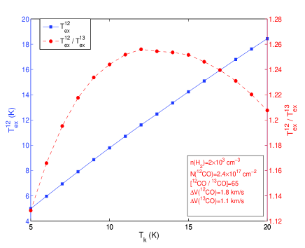
The LTE assumption is another crucial factor of the uncertainties in determining the column density. In non-LTE case, the excitation temperature of the 13CO (1-0) and C18O (1-0) lines may be very different from that of 12CO (1-0) (Liu et al., 2012a). We applied RADEX (van der Tak et al., 2007), a one-dimensional non-LTE radiative transfer code, to investigate the effect of non-LTE on the determination of column density of 13CO. The median value of 13CO column density under LTE assumption is 3.7 cm-2. The median values of the linewidth of 13CO (1-0) and 12CO (1-0) are 1.1 and 1.8 km s-1, respectively. We fix the volume density of H2 as 2.0 cm-3, which is the mean value of the whole C3PO sample (Planck Collaboration. et al., 2011). Taking the typical values mentioned above and assuming that the relative abundance of 12CO to 13CO is 65, we simulated the emission of 12CO (1-0) and 13CO (1-0) in a parameter space for the kinetic temperature of [5,20] K using LVG model in RADEX.
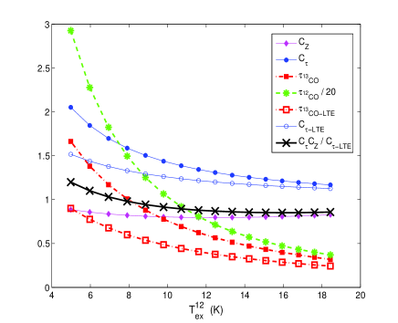
In the left panel of Figure 1, we plot the excitation temperature of 12CO (1-0) and the ratio of the excitation temperature of 12CO (1-0) to that of 13CO (1-0) as a function of the kinetic temperature . There is a linear relation between the the excitation temperature of 12CO (1-0) and the kinetic temperature: . The ratio of to ranges from 1.13 to 1.26 with a mean value of 1.22, indicating that the LTE assumption overestimates the excitation temperature of 13CO (1-0) by a factor of 20%. This leads to an underestimation of the 13CO (1-0) opacity which in turn affects the opacity correction of the column density. From the right panel of Figure 1, one can see that the optical depth of 12CO (1-0) decreases with the kinetic temperature but is much larger than 1. The optical depth of 13CO (1-0) calculated with RADEX also decreases with the kinetic temperature. At low kinetic temperature (8 K), the 13CO (1-0) emission may become optically thick. We also noticed that the optical depth of 13CO (1-0) calculated with RADEX is larger than that calculated under LTE assumption, especially at low kinetic temperatures. Therefore the opacity correction factor under non-LTE condition should be larger than . However, the overestimation of the excitation temperature not only affect the optical depth but also affect the partition function. The partial function Z is given by
| (5) |
Thus the correction factor on Z due to non-LTE can be defined as . Where and are the excitation temperatures of 13CO (1-0) and 12CO (1-0), respectively. In the right panel of Figure 1, we plot and as function of . We find that is smaller than 1. is larger than 1 at lower temperature end, while smaller than 1 at high temperature end. However, varies slightly around 1 by a factor less than 20%, indicating that the uncertainty in the estimation of column density due to non-LTE effect is less than 20%. For this reason, we use the column density estimated under LTE assumption in the following analysis.
The total column density of H2 () can be calculated with (Planck Collaboration. et al., 2011)
| (6) |
where Sν is the flux density at 857 GHz integrated over the solid angle with and the major and minor axis of the source, is the Planck function at temperature T, is the mean molecular weight, and is the mass of atomic hydrogen. The dust opacity =0.1(/1 THz)β cm2g-1, with the dust emissivity spectral index (Planck Collaboration. et al., 2011).
The mass of the clumps are calculated as (Planck Collaboration. et al., 2011)
| (7) |
where Sν is the integrated flux density at 857 GHz, D is the distance.
The Bolometric luminosity is defined by (Planck Collaboration. et al., 2011)
| (8) |
where Sν is the flux density at frequency . The bolometric luminosity, L, is integrated over the frequency range 300 GHz 10 THz, using the modelled SEDs (Planck Collaboration. et al., 2011). The luminosity-to-mass ratio of the clumps ranges from to 3.5 L☉/M☉, with a median value of 0.2 L☉/M☉, indicating the Planck cold clumps are not significantly affected by star forming activities.
The averaged volume density is defined by
| (9) |
The resulting volume density ranges from to cm-3, with a mean value of 5.4 cm-3, which is slightly larger than the mean value (2 cm-3) of the whole C3PO sample (Planck Collaboration. et al., 2011).
If 12CO (1-0) emission has corresponding C18O (1-0) emission, the column density of 12CO () is converted from with the 16O/18O isotope ratio as (Wilson & Rood, 1994)
| (10) |
where R is the Galactocentric distance.
Otherwise, we converted to using the isotope ratio given by (Pineda et al., 2013)
| (11) |
The above relationship gives a 12C/13C isotope ratio of 65 at R=8.5 kpc.
In the sample, about 30% clumps have double or multiple velocity components in 12CO emission and 16% have double or multiple velocity components in 13CO emission (Wu et al., 2012). We only considered the velocity components having 13CO emission in the calculation of the abundance. The observed 12CO abundance is [12CO/H2]=, where i denotes the number of the 13CO velocity components of each source. One should keep in mind that in the calculation we assume the dust emission is uniform in the clumps, which may be not the case because in our CO mapping survey (Liu, Wu & Zhang, 2012) and Herschel follow-up surveys (Juvela et al., 2010, 2012) most of the Planck clumps have sub-structures. This insufficiency can be improved in future by comparing the CO maps with the dust emission maps obtained from higher resolution observations (e.g. Herschel or ground-based telescopes like APEX).
The median and mean values of the observed gaseous 12CO abundance are 0.89 and 1.28, respectively.
3.2 CO depletion and CO-to-H2 conversion factor
The CO depletion factor, , is defined as:
| (12) |
where is the ’expected’ abundance of CO.
Taking into account the variation of atomic carbon and oxygen abundances with the Galactocentric distance, the expected 12CO abundance at the Galactocentric distance R of each source is (Fontani et al., 2012):
| (13) |
This relationship gives a canonical CO abundance of in the neighborhood of the solar system (Frerking, Langer & Wilson, 1982; Langer et al., 1989; Pineda, Caselli & Goodman, 2008).
The mean and median of CO depletion factor are 1.7 and 0.9, respectively. About 53% Planck cold clumps have CO depletion factor smaller than 1. Only 13% Planck cold clumps have CO depletion factor larger than 3 and Only about 5.6% larger than 5. It seems that the CO gas in Planck cold clumps is not severely depleted. And due to the large beam size of PMO 13.7 m telescope and Planck satellite, we can not separate the depleted gas from the non-depleted gas, which should influence the interpretation of the CO depletion measurements. Thus our measurements indicate that on clump scale the CO depletion is not significant, in agreement with the fact that on such scales the observed emission arise mostly from low-density, non-depleted gas.
The CO-to-H2 conversion factor , with the integrated intensity of the 12CO (1-0) line. The median value of for the whole sample is cm-2K-1km-1 s. However, CO emission may be saturated at high column density, which will add uncertainties in measuring . Within the Perseus molecular cloud, the 12CO emission saturates at 4 mag (Pineda, Caselli & Goodman, 2008). If we only consider the Planck cold clumps with 4 mag (N cm-2), the median and mean values of are 1.7 and 1.9 cm-2K-1km-1 s, respectively, which are in agreement with the mean value of (1.8 cm-2K-1km-1 s for the Milky Way (Dame, Hartmann & Thaddeus , 2001).
4 Discussion
4.1 The relationships between various physical parameters
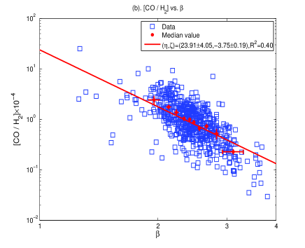
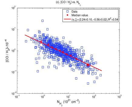
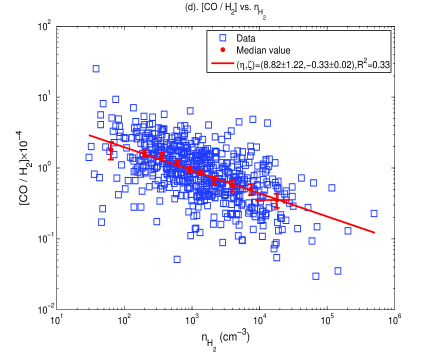
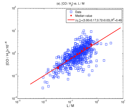
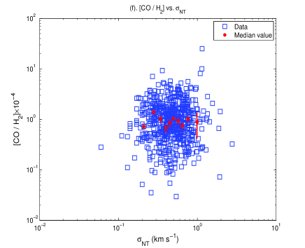
In Figure 2, we investigate the relationships between CO abundance and dust temperature (Td), dust emissivity spectral index (), column density of H2 (N), volume density of H2 (n), luminosity-to-mass ratio (L/M) as well as the non-therm one dimensional velocity dispersion (). CO abundance strongly correlates with Td and L/M and anti-correlates with , N and n. These relationships were well fitted with a power-law function (). The coefficients of each model as well as the correlation coefficients are displayed in the upper-right corner of each panel. There is no correlation between CO abundance and , indicating that turbulence has no effect on the fluctuation of CO abundance. The lower CO abundance for the clumps with lower Td and with higher N or n indicates that CO gas may freeze out significantly towards cold and dense regions. The growth of icy mantles on dust grains could steepen the slope of the dust SED and thus increase the emissivity spectral index (Schnee et al., 2010). The anti-correlation between CO abundance and indicates that huge amount of gaseous CO transforms to icy CO with the growth of icy mantles on dust grains. However, the presence of observational errors makes the anti-correlation between the Td and become unreliable in the C3PO sample (Planck Collaboration. et al., 2011). Thus the relationships between and the other physical parameters should be taken seriously and tested by further more detailed observations.
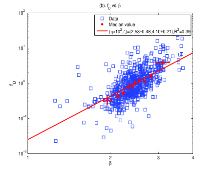
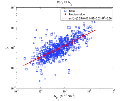
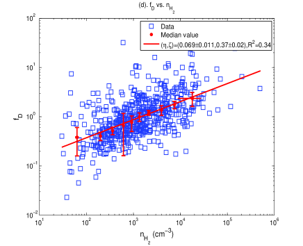
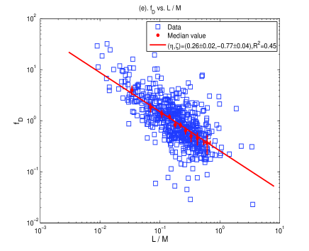
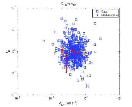
In Figure 3, we plot the CO depletion factor fD as a function of Td, , N, n, L/M and . The fD significantly anti-correlates with Td and L/M and positively correlates with , N and n. These relationships were well fitted with a power-law function (). In each panel, we divide the data into ten bins and plot median fD in each bin as red filled circles. We find that the median fD is larger than 1 in bins with T10.8 K or or N6.6 cm-2 or n1.7 cm-3 or L/M0.16, indicating that CO gas freeze out in cold and dense regions without significant internal heating. There is also no correlation between CO depletion factor fD and .
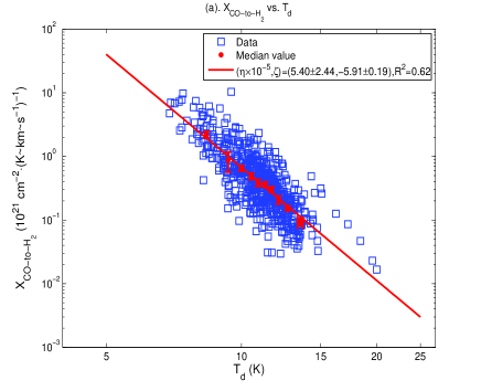
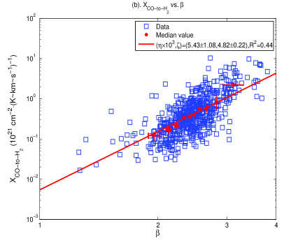
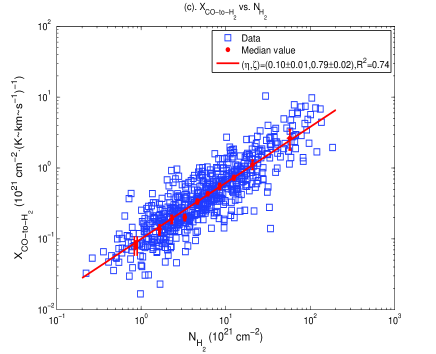
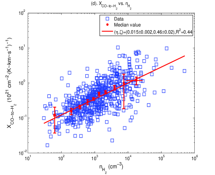
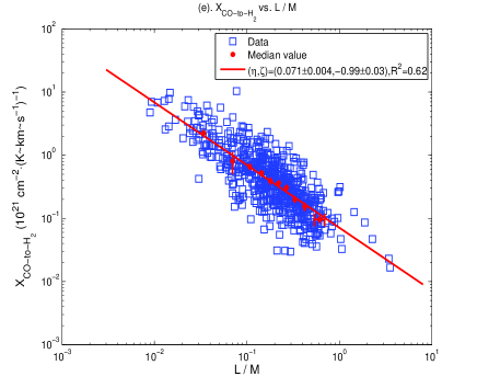
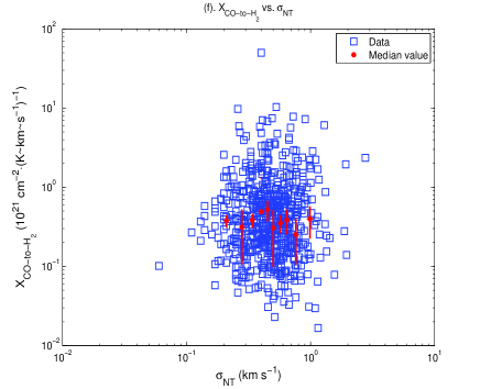
The variation of gaseous CO abundance in molecular clouds should seriously hamper its utility as an estimator of the total hydrogen column density. In Figure 4, we plot the CO-to-H2 conversion factor against Td, , N, n, L/M and . In each panel, the median values of in each bin are plotted as red filled circles. There is an inverse correlation between and Td and L/M. While positively correlates to , N and n. These relationships can be well fitted with power-law functions. There is no correlation between and . We found that the median value of is larger than 2 cm-2K-1km-1 s in bins with T12 K or or N2.6 cm-2 or n2.8 cm-3 or L/M0.34.
4.2 Gaseous CO abundance — An evolutionary tracer for molecular clouds
The freezing out of gaseous CO onto grain surfaces strongly influences the physical and chemical properties of molecular clouds. As a major destroyer of molecular ions, the CO depletion leads to a change in the relative abundances of major charge carriers (e.g.H, N2H+ and HCO+) and thus causes variation in the ionizing degree (Caselli et al., 1999; Bergin & Tafalla, 2007). Another second-effect induced by CO depletion is deuterium enrichments in cold cores (Caselli et al., 1999; Bergin & Tafalla, 2007). These effects make gaseous CO abundance a promising tool to time the evolution of molecular clouds. As discussed in section 1, significant fraction of CO molecules is transformed from gas to solid as the gas density increases (Hernandez et al., 2011; Whittet, Goldsmith & Pineda, 2010). As molecular clump evolves, the density and temperature increase. The bolometric luminosity also increases as the protostars form and evolve in molecular clumps (Emprechtinger et al., 2009). The ratio of bolometric luminosity to submillimeter emission is also used as an effective indicator for protostar evolution. In this work, we found that the relative abundance of gaseous CO significantly anti-correlates with dust temperature and luminosity-to-mass ratio and positively correlates with column density, volume density and dust emissivity spectral index, indicating that gaseous CO abundance can also well serve as an evolutionary indicator.
One should keep in mind that the Planck cold clumps are cold ( K) (Planck Collaboration. et al., 2011), turbulence dominated and have relatively low column densities comparing with the other star forming regions (Wu et al., 2012). They are mostly quiescent and lacking star forming activities, indicating that the Planck cold clumps are most likely at the very initial evolutionary stages of molecular clouds (Wu et al., 2012). Thus the relationships between various physical parameters reported here may be only valid for molecular clouds without significant star forming activities. However, our results indicate that gaseous CO abundance (or depletion) can be used as a tracer for the evolution of molecular clouds. Actually, people have already used CO depletion to distinguish relatively evolved starless cores from more-recently condensed cores (Tafalla & Santiago, 2004; Tafalla , 2010).
Acknowledgment


References
- Bergin & Tafalla (2007) Bergin, E. A. & Tafalla, M., 2007, ARA&A, 45, 339
- Caselli et al. (1999) Caselli, P., Walmsley, C. M., Tafalla, M., Dore, L., Myers, P. C., 1999, ApJ, 523, L165
- Christie et al. (2012) Christie, H., Viti, S., Yates, J., Hatchell, J., Fuller, G. A. et al., 2012, MNRAS, 422, 968
- Dame, Hartmann & Thaddeus (2001) Dame, T. M., Hartmann, D., & Thaddeus, P. 2001, ApJ, 547, 792
- Emprechtinger et al. (2009) Emprechtinger, M., Caselli, P., Volgenau1, N. H., Stutzki, J., & Wiedner, M. C., 2009, A&A, 493, 89
- Fontani et al. (2012) Fontani, F., Giannetti, A., Beltrán, M. T., Dodson, R., Rioja, M., Brand, J., Caselli, P., Cesaroni, R., 2012, MNRAS, 423, 2342
- Frerking, Langer & Wilson (1982) Frerking, M., Langer, L., Wilson, R. 1982, ApJ, 262, 590
- Garden et al. (1991) Garden, R. P., Hayashi, M., Hasegawa, T., Gatley, I., Kaifu, N., 1991, ApJ, 374, 540
- Hernandez et al. (2011) Hernandez, A. K., Tan, J. C., Caselli, P., Butler, M. J., Jiménez-Serra, I., Fontani, F., Barnes, P., 2011, ApJ, 738, 11
- Juvela et al. (2010) Juvela, M., Ristorcelli, I., Montier, L. A., et al. 2010, A&A, 518, L93
- Juvela et al. (2012) Juvela, M., Ristorcelli, I., Pagani, L., et al. 2012, A&A, 541, A12
- Kramer et al. (1999) Kramer, C., Alves, J., Lada, C. J., Lada, E. A., Sievers, A., Ungerechts, H., & Walmsley, C. M. 1999, A&A, 342, 257
- Langer et al. (1989) Langer, W. D., Wilson, R. W., Goldsmith, P. F., & Beichman, C. A. 1989, ApJ, 337, 355
- Liu et al. (2012a) Liu, T., Wu, Y., Zhang, H., Qin, S.-L., 2012a, ApJ, 751, 68
- Liu, Wu & Zhang (2012) Liu, T., Wu, Y., Zhang, H., 2012b, ApJS, 202, 4
- Pillai et al. (2007) Pillai, T., Wyrowski, F., Hatchell, J., Gibb, A. G. & Thompson, M. A., 2007, A&A, 467, 207
- Pineda, Caselli & Goodman (2008) Pineda, J. E., Caselli, P. & Goodman, A. A., 2008, ApJ, 679, 481
- Pineda et al. (2010) Pineda, J. L., Goldsmith, P. F., Chapman, N., Snell, R. L., Li, D., Cambrésy, L., Brunt, C. 2010, ApJ, 721, 686
- Pineda et al. (2013) Pineda, J. L., Langer, W. D., Velusamy, T., Goldsmith, P. F., 2013, accepted to A&A, arXiv:1304.7770
- Planck Collaboration. et al. (2011) Planck Collaboration., Ade, P. A. R., Aghanim, N., Arnaud, M., Ashdown, M., et al., 2011, A&A, 536, 23
- Rodríguez et al. (1982) Rodríguez, L. F., Carral, P., Moran, J. M., & Ho, P. T. P. 1982, ApJ, 260, 635
- Schnee et al. (2010) Schnee, S., Enoch, M., Noriega-Crespo, A., Sayers, J., Terebey, S., et al. 2010, ApJ, 708, 127
- Tafalla et al. (2002) Tafalla, M., Myers, P. C., Caselli, P., Walmsley, C. M., Comito, C., 2002, ApJ, 569, 815
- Tafalla & Santiago (2004) Tafalla, M., & Santiago, J. 2004, A&A, 414, L53
- Tafalla (2010) Tafalla, M., Highlights of Spanish Astrophysics VI, Proceedings of the IX Scientific Meeting of the Spanish Astronomical Society (SEA), held in Madrid, September 13-17, 2010, Eds.: M. R. Zapatero Osorio, J. Gorgas, J. Ma z Apell niz, J. R. Pardo, and A. Gil de Paz., p. 442-453
- van der Tak et al. (2007) van der Tak, F.F.S., Black, J.H., Schöier, F.L., Jansen, D.J., van Dishoeck, E.F. 2007, A&A, 468, 627
- Wilson & Rood (1994) Wilson, T. L., & Rood, R. T. 1994, ARA&A, 32, 191
- Whittet, Goldsmith & Pineda (2010) Whittet, D. C. B., Goldsmith, P. F., & Pineda, J. L., 2010, ApJ, 720, 259
- Wu et al. (2004) Wu, Y., Wei, Y., Zhao, M., Shi, Y., Yu, W., Qin, S., Huang, M., 2004, A&A, 426, 503
- Wu et al. (2012) Wu, Y., Liu, T., Meng, F., Li, D., Qin, S.-L., Ju, B.-G., 2012, ApJ, 756, 76