Young Stellar Clusters with a Schuster Mass Distribution - I: Stationary Winds

Abstract

Hydrodynamic models for spherically-symmetric winds driven by young stellar clusters with a generalized Schuster stellar density profile are explored. For this we use both semi-analytic models and 1D numerical simulations. We determine the properties of quasi-adiabatic and radiative stationary winds and define the radius at which the flow turns from subsonic into supersonic for all stellar density distributions. Strongly radiative winds diminish significantly their terminal speed and thus their mechanical luminosity is strongly reduced. This also reduces their potential negative feedback into their host galaxy ISM. The critical luminosity above which radiative cooling becomes dominant within the clusters, leading to thermal instabilities which make the winds non-stationary, is determined, and its dependence on the star cluster density profile, core radius and half mass radius is discussed.

1 Introduction

The feedback from massive young stellar clusters to the interstellar gas determines the natural link between the stellar and gaseous components in galaxies. High velocity gaseous outflows driven by young stellar clusters (star cluster winds) shape the interstellar medium (ISM) into a network of expanding shells that engulf a hot X-ray emitting plasma (Wang et al., 2010). Such shells accumulate and compress the interstellar matter often creating secondary star forming clumps within the expanding shells (Oey et al., 2005) and massive young stellar systems in sites of shell collisions, as it seems to be the case of 30 Dor and other regions in the Large Magellanic Cloud (Dawson et al., 2013; Book et al., 2009). A number of massive young stellar clusters are found in interacting and starburst galaxies (Portegies Zwart et al., 2010), where the thermalization of the kinetic energy supplied by massive stars may result in powerful, galactic scale outflows, which link the central starburst zone of galaxies with the low density galactic gaseous halo and the intergalactic medium (Tenorio-Tagle & Muñoz-Tuñón, 1998; Tenorio-Tagle et al., 2003).

Theoretical models dealing with such outflows, assumed either that the energy is released in the system center, or that stars are homogeneously distributed within the star cluster volume, as suggested in the pioneer work by Chevalier & Clegg (1985). The discussion of winds driven by clusters with different stellar density distributions is rather incomplete: Rodríguez-González et al. (2007) found an analytic non-radiative solution in the case of a power law stellar density distributions and compared it with 3D simulations. Ji et al. (2006) presented results from 1D numerical simulations of non-radiative winds driven by stellar clusters with an exponential stellar density distributions. The impact of radiative cooling on winds driven by stellar clusters with an exponential stellar density distribution is discussed in Silich et al. (2011), who developed a semi-analytic method, which allows to localize the position of the singular point where the flow turns from subsonic to supersonic and calculate the run of all hydrodynamical variables in this case.

The observed star cluster brightness profiles, however, are different from those discussed in all above studies. In most cases a generalized Schuster density profile with $\rho_{*}\propto[1+(r/R_{c})^{2}]^{-\beta}$ with $\beta=1.5$, where $R_{c}$ is the core radius of the cluster stellar distribution, provides the best fit to the empirical mass distribution in young stellar clusters (Veltmann, 1979). Whitworth & Ward-Thompson (2001) used this profile to describe the distribution of pre-stellar cores (PSC) in their model of forming clusters. Dib et al. (2007) adopted this distribution to PSC and young stars in the Arches cluster near the center of the Milky Way. Elson et al. (1987) revealed that the generalized Schuster model with $\beta=1.75$, provides a very good fit to the stellar densities of young stellar clusters in the Large Magellanic Cloud. Furthermore, Mengel et al. (2002) used HST observations of young stellar clusters in the Antennae galaxies (Whitmore et al., 1999), and found that a King model (King, 1962, 1966) provides the best agreement with the observed stellar surface densities, corresponding to a generalized Schuster model.

The adiabatic model of winds driven by clusters with a homogeneous stellar density distribution by Chevalier & Clegg (1985, hereafter CC85) complemented with the effects of radiative cooling were explored by Silich et al. (2004), Tenorio-Tagle et al. (2007), Wünsch et al. (2007), Wünsch et al. (2008), Tenorio-Tagle et al. (2010), and Wünsch et al. (2011). They concluded that the importance of cooling increases for larger mass clusters. For a given cluster radius, when the cluster mass surpasses a critical value, the stationary wind solution vanishes.

Here we extend our previous results to clusters with a generalized Schuster profile and discuss how it affects the hydrodynamics of star cluster winds. One can use the results presented here, as a reference model, and compare them with the observed systems. This might improve the link between observations and model predictions, help in the interpretation of observational data and improve our understanding of the stellar feedback and the fraction of stellar mass returned to the galactic ISM.

The paper is organized as follows: the input star cluster model is formulated in section 2. In section 3 we introduce the set of main equations and present them in the form suitable for numerical integration in the semi-analytic approach. The numerical model is presented in section 4. Reference models are described in section 5, where the results obtained with different methods are compared. We discuss separately the non-radiative solutions and the stationary radiative solutions through a detailed comparative description of models obtained with different energies. We summarize our major results in section 6. The non-stationary solutions including thermal instabilities will be discussed in a forthcoming communication (Wünsch et al., 2013).

2 Input model

We consider young and compact spherical clusters with constant total mass and energy deposition rates, $\dot{M}_{SC}$ and $L_{SC}$, and a generalized Schuster stellar mass density distribution (Ninkovic, 1998):

$$\rho_{\star}(r)=\displaystyle\frac{\rho_{\star 0}}{\left[1+\left(r/R_{c}\right)^{2}\right]^{\beta}},$$ (1)

where $\rho_{\star 0}$ is the central stellar density, $R_{c}$ is the radius of the star cluster “core” and $\beta\geq 0$ defines the steepness of the stellar distribution. The cumulative mass within a given radius $r$ is then:

$$M_{SC}(r)=\displaystyle\int_{0}^{r}\frac{4\pi\rho_{*0}x^{2}{\rm d}x}{\left[1+\left(x/R_{c}\right)^{2}\right]^{\beta}}=\frac{4\pi}{3}\rho_{*0}r^{3}{}_{2}F_{1}(3/2,\beta,5/2,-r^{2}/R_{c}^{2}),$$ (2)

where ${}_{2}F_{1}$ is the Gauss hypergeometric function, ${}_{2}F_{1}(3/2,\beta,5/2,-r^{2}/R_{c}^{2})$, hereafter abbreviated as $F_{\beta}(r)$.

If $\beta\leq 3/2$ and $r\rightarrow\infty$, the mass of the cluster is infinite. However, if $\beta>3/2$, the cumulative mass is finite even if $r\to\infty$. In order to keep the cluster total mass finite even for $\beta\leq 3/2$, the stellar density distribution (equation 1) must be truncated at some radius $R_{SC}$. The consideration of the cluster radius $R_{SC}$ is justified as a consequence of environmental effects, tides etc., which remove mass from the cluster periphery. When $\beta=3/2$ and $R_{SC}/R_{c}\to\infty$, equation (1) leads to the King (1962) surface density distribution (Ninkovic, 1998). Note, that in the case of a homogeneous stellar mass distribution ($\beta=0$) the core radius $R_{c}$ vanishes from all formulae.

Here it is assumed, as in CC85, that the mechanical energy deposited by massive stars and supernova explosions is thermalized in random collisions of nearby stellar winds and supernova ejecta and that sources of mass ($q_{m}$) and energy ($q_{e}$) are distributed in direct proportion to the local star density:

$$q_{e}(r)=\displaystyle q_{e0}\left[1+\left(r/R_{c}\right)^{2}\right]^{-\beta},$$ (3)

, $$q_{m}(r)=\displaystyle q_{m0}\left[1+\left(r/R_{c}\right)^{2}\right]^{-\beta},$$ (4)

where the normalization constants $q_{e0}$ and $q_{m0}$ are:

$$q_{e0}=\displaystyle 3L_{SC}/4\pi R_{c}^{3}F_{\beta}(R_{SC}),$$ (5)

$$q_{m0}=\displaystyle 3\dot{M}_{SC}/4\pi R_{c}^{3}F_{\beta}(R_{SC}).$$ (6)

3 Semi-analytic approach

3.1 Basic equations

The hydrodynamic equations for the steady state, spherically symmetric flows driven by clusters with energy and mass deposition rates $q_{e}(r)$ and $q_{m}(r)$ are (see, for example, Johnson & Axford, 1971; Chevalier & Clegg, 1985; Cantó et al., 2000; Silich et al., 2004):

$$\frac{1}{r^{2}}\frac{{\rm d}}{{\rm d}r}\left(\rho ur^{2}\right)=q_{m},$$ (7)

$$\rho u\frac{{\rm d}u}{{\rm d}r}=-\frac{{\rm d}p}{{\rm d}r}-q_{m}u,$$ (8)

$$\frac{1}{r^{2}}\frac{{\rm d}}{{\rm d}r}{\left[\rho ur^{2}\left(\frac{u^{2}}{2}+\frac{\gamma}{\gamma-1}\frac{p}{\rho}\right)\right]}=q_{e}-Q,$$ (9)

where $u$, $p$, and $\rho$ are the gas outflow velocity, thermal pressure and density, respectively, $\gamma$ (=5/3) is the ratio of the specific heats, $Q=n_{e}n_{i}\Lambda(T,Z)$ is the cooling rate, $n_{e}$, $n_{i}$ are the number densities of electrons and ions, and $\Lambda(T,Z)$ is the cooling function, which depends on the gas temperature $T$ and metallicity $Z$. We use the equilibrium cooling function for optically thin plasma obtained by Plewa (1995). In all calculations the metallicity of the plasma was set to the solar value. Hereafter we relate the energy and the mass deposition rates, $L_{SC}$ and ${\dot{M}}_{SC}$, via the equation:

$$L_{SC}={\dot{M}}_{SC}V^{2}_{A\infty}/2,$$ (10)

and assume that the adiabatic wind terminal speed, $V_{A\infty}$, is constant. For a known star cluster mechanical luminosity $L_{SC}$, the parameter $V_{A\infty}$ defines the mass deposition rate.

The integration of the mass conservation equation (7) yields:

$$\rho ur^{2}=q_{m0}r^{3}F_{\beta}(r)/3+C.$$ (11)

If the density and the velocity of the flow in the star cluster center are finite, the constant of integration must be zero: $C=0$. Using this expression and taking the derivative of equation (9), one can present the main equations in a form suitable for numerical integration:

$$\frac{{\rm d}u}{{\rm d}r}=\frac{\displaystyle(\gamma-1)(q_{e}-Q)+(\gamma+1)q_{m}u^{2}/2-2c^{2}\rho u/r}{\displaystyle\rho(c^{2}-u^{2})},$$ (12)

$$\frac{{\rm d}p}{{\rm d}r}=-\rho u\frac{{\rm d}u}{{\rm d}r}-q_{m}u\,,$$ (13)

$$\rho=\frac{q_{m0}r}{3u}F_{\beta}(r)\,,$$ (14)

where $c$ is the local speed of sound, $c^{2}=\gamma p/\rho$.

Given a cluster radius $R_{SC}$, outside of which there are no sources of mass and energy, the set of the main equations for $r>R_{SC}$ is:

$$\frac{{\rm d}u}{{\rm d}r}=\frac{(\gamma-1)rQ+2\gamma pu}{r\rho(u^{2}-c^{2})},$$ (15)

$$\frac{{\rm d}p}{{\rm d}r}=-\frac{{\dot{M}}}{4\pi r^{2}}\frac{{\rm d}u}{{\rm d}r}\,,$$ (16)

$$\rho=\frac{{\dot{M}}}{4\pi ur^{2}}\,,$$ (17)

where $\dot{M}$ is the flux of mass through the star cluster surface.

3.2 Integration procedure

As a consequence of equation (14) the central gas density $\rho_{0}$ is non zero and remains finite only if the flow velocity at $r=0$ is zero, and grows linearly with radius near the center. The derivatives of the wind velocity and pressure in the star cluster center then are:

$$\frac{{\rm d}u}{{\rm d}r}=\left[(\gamma-1)(q_{e0}-Q)-2q_{m0}c_{0}^{2}/3\right]/\rho_{0}c^{2}_{0}\,,$$ (19)

$$\frac{{\rm d}p}{{\rm d}r}=0\,,$$

where $c_{0}$ is the sound speed in the star cluster center. It is interesting to note, that these relations are identical to those, obtained for the top-hat or homogeneous and for the exponential stellar density distribution by Silich et al. (2004, 2011), and that they do not depend on the selected value of $\beta$. We make use of these equations in order to move from the center and start the numerical integration.

In the radiative wind model, the central gas density $\rho_{0}$ and the central temperature $T_{0}$ are related through the equation (Sarazin & White, 1987; Silich et al., 2004):

$$n_{0}=q_{m0}^{1/2}\left[\frac{V_{A,\infty}^{2}/2-c_{0}^{2}/(\gamma-1)}{\Lambda(Z,T_{0})}\right]^{1/2}\,$$ (20)

where $n_{0}=\rho_{0}/\mu m_{p}$ is the central number density of ions and $\mu m_{p}$ is the average mass per ion. Thus the central temperature $T_{0}$ is the only parameter which selects the solution from a branch of possible integral curves.

Searching for the physical wind solution, two cases may occur. In the first one, it is possible to find the unique solution which passes through the singular point $R_{sg}$, where both, the numerator and the denominator in equation (12) vanish inside of the cluster: $R_{sg}<R_{SC}$. At this point, the subsonic flow in the region $r<R_{sg}$ changes to a supersonic flow in the region $r>R_{sg}$, thus the singular point is also the sonic point. The presence of $R_{sg}$ inside the cluster allows one to select the value of the central temperature and the unique wind solution. The position of the singular point $R_{sg}$ can be calculated using the method described by Silich et al. (2011), where the formulae which define the hydrodynamic variables and the derivative of the flow velocity at $R_{sg}$, and which allow to pass it in the semi-analytic calculations, are given.

In the other case, if the singular point does not exist inside the cluster, the transition from a subsonic to a supersonic flow occurs abruptly at $R_{SC}$, where the stellar density changes discontinuously and where the velocity gradient is infinite, CC85 and Cantó et al. (2000). In this case the numerator and denominator of equation (12) are both positive when one approaches $R_{SC}$ from the inside, and both negative when one approaches it from the outside.

4 Numerical simulations

We perform 1D numerical simulations to complement the semi-analytical calculations and confirm the results. Full numerical simulations are also required in order to find the hydrodynamic solution in the case of very energetic clusters, where strong radiative cooling promotes thermal instabilities and inhibits a stationary solution. The models are calculated with the finite-difference Eulerian hydrodynamic code FLASH (Fryxell et al., 2000). Here we perform the 1D numerical simulations assuming spherically symmetric clusters. The calculation of radiative cooling within the computational domain and its impact on the time-step is computed following Tenorio-Tagle et al. (2007, hereafter GTT07) and Wünsch et al. (2008, hereafter W08), where the cooling routine uses the Raymond et al. (1976) cooling function updated by Plewa (1995).

In GTT07 and W08 the flow was modeled considering a continuous replenishment of internal energy and mass in all cells within the cluster volume at rates $q_{e}(r)$ and $q_{m}(r)$, respectively. The dependence of these quantities on radius is given by equations (3) and (4) with the normalization constants given by equations (5) and (6). $\dot{M}_{SC}$ is related to $L_{SC}$ as given by equation (10) through the constant $V_{A\infty}$, thus defining the mass flux in the cluster wind. Small values of $V_{A\infty}$ mean that the mass in winds of individual stars is loaded by additional mass from the parental cloud. At every time-step energy and mass are inserted within the cluster volume following the procedure described in GTT07 and W08.

5 Results and discussion

5.1 Non-radiative winds

For a stationary wind the total energy flux $L(r)$ through a sphere of radius $r$ is:

$$L(r)\equiv 4\pi r^{2}\rho u(\frac{u^{2}}{2}+\frac{\gamma}{\gamma-1}\frac{p}{\rho})\ .$$ (21)

In the non-radiative case, this has to be equal to the energy

$$L(r)=\int_{0}^{r}4\pi x^{2}q_{e}dx=4\pi r^{3}F_{\beta}(r)/3$$ (22)

inserted by stars into a sphere with the same radius. At the sonic point $R_{son}$, the wind velocity fulfills $u(R_{son})=c(R_{son})$ which together with equations (21) and (22) and the sound speed definition $c^{2}=\gamma p/\rho$ yields

$$3\rho c^{3}(\gamma+1)=2(\gamma-1)q_{e0}R_{son}F_{\beta}(R_{son}).$$ (23)

Inserting the continuity equation (14) into (23) and utilizing $V_{A\infty}^{2}=2q_{e0}/q_{m0}$ one gets

$$c^{2}(R_{son})=\frac{\gamma-1}{\gamma+1}V_{A\infty}^{2}.$$ (24)

This implies that in the adiabatic case ($Q=0$), the sound speed at the sonic point $R_{son}$, is exactly one half of the terminal wind velocity $V_{A\infty}$, if $\gamma=5/3$ (see Cantó et al., 2000).

Figure 1: The position of the singular point $R_{sg}$ normalized by the core radius $R_{c}$ as a function of $\beta$. Solid line shows the solution of the equation (26), x symbols give the position of the sonic points measured in 1D hydrodynamical simulations. The vertical dotted line marks the limiting $\beta$ value $\beta_{crit}$ for which the singular point goes to infinity.

When the transition to the supersonic regime occurs inside the cluster, the denominator and the numerator of equation (12) are both equal to zero and $R_{son}=R_{sg}$. In the non-radiative case ($Q=0$) it leads to:

$$(\gamma-1)q_{e}+(\gamma+1)q_{m}\frac{c}{2}-\frac{2}{3}q_{m0}c^{2}F_{\beta}(R_{sg})=0.$$ (25)

Equations (3), (4) and (24) then lead to the algebraic equation for $R_{sg}$

$$\left[1+\left(\frac{R_{sg}}{R_{c}}\right)^{2}\right]^{-\beta}=\frac{4}{3(5\gamma-3)}F_{\beta}(R_{sg})\ .$$ (26)

The solution of equation (26) can be found numerically. It is a function of only one parameter ($\beta$). The position of the adiabatic singular point for all clusters with a Schuster stellar density profile is shown in Figure 1, where the solution of equation (26) is also compared to the sonic point positions measured in 1D hydrodynamic simulations. There is an excellent agreement between the two methods. The dependence on the sources (stellar) density distribution alone was already claimed by Ji et al. (2006).

It is important to note, that in the adiabatic case (when Q = 0) there is a critical value of $\beta$ ($\beta_{crit}=1.125$) such that for $\beta\leq\beta_{crit}$ the singular point $R_{sg}\to\infty$. This implies, that in clusters with a shallow stellar density distributions ($\beta\leq\beta_{crit}$), the transition to the supersonic regime occurs at infinity (see Figure 1), or if truncated, at the star cluster surface $R_{SC}$. On the other hand, in clusters with steeper density gradients the transition to the supersonic regime occurs inside the cluster, if the star cluster is sufficiently large: $R_{SC}>R_{sg}$.

5.2 Reference models

Figure 2: Stationary wind solution for quasi-adiabatic winds. The wind velocity $u$ - thick lines and the sound speed $c$ - thin lines (upper left), the density $n$ (upper right), the temperature $T$ (lower left) and the thermal pressure $p/k_{B}$ (lower right) are shown. $k_{B}$ is the Boltzmann constant. The lines present the results from the semi-analytic calculations and the circle symbols give the results of 1D hydrodynamical simulations: Model I (dotted lines), Model II (dashed lines), Model III (dash-dotted lines), Model IV (solid lines). The transition to a supersonic regime occurs at radii, where on the left upper panel the thin and thick lines of the corresponding model cross.

Table 1: Reference models

Model	$\beta$	Core radius	Cluster radius	Sonic radius
		$R_{c}$(pc)	$R_{SC}$(pc)	$R_{son}$(pc)
(1)	(2)	(3)	(5)
I	0	…	3.36	3.36
II	1.0	1.176	4.14	4.14
III	1.5	1.176	5.59	5.34
IV	2.0	1.176	$\infty$	2.78

The input parameters for our reference models are presented in Table 1. All reference clusters (Models I, II, III and IV) include radiative cooling (see equations 9, 12 and 15) and have the same half-mass radius as the exponential model of Silich et al. (2011): $R_{hm}=2.67$ pc and the same adiabatic wind terminal speed: $V_{A\infty}=1000$ km s^-1. For Model I, which has the flat top-hat stellar density profile ($\beta=0$), the value of the cut-off radius is $R_{SC}=3.36$ pc. The core radius ($R_{c}=1.176$ pc) was chosen so that for $\beta=2$ the half mass radius is $R_{hm}=2.67$ pc with $R_{SC}\rightarrow\infty$. We use the same value of $R_{c}=1.176$ pc in models II and III, what leads to the star cluster radii $R_{SC}=4.14$ pc and $R_{SC}=5.59$ pc, respectively.

First, we computed the hydrodynamic variables in our reference Models I - IV as functions of $r$ for a mechanical luminosity $L_{SC}=3\times 10^{40}$ erg/s, which is typical for young stellar clusters with masses $\sim$ $10^{6}$  $\hbox{M}_{\odot}$. For this mechanical luminosity radiative cooling is not important and all the models behave quasi-adiabatically. Figure 2 shows the distributions of the flow velocity and sound speed (upper left panel), density (upper right panel), temperature (lower left panel) and thermal pressure (lower right panel). The lines show the results from the semi-analytic calculations, whereas circle symbols give the hydrodynamic variables obtained in 1D simulations. The results from the semi-analytic and 1D simulations are in an excellent agreement.

If the transition to the supersonic regime occurs at the star cluster surface, as in the case of Models I and II, the velocity jumps abruptly from subsonic to supersonic, and the density, temperature and pressure decrease sharply at the cluster edge. If the sonic point resides inside the cluster, as in Models III and IV, the transitions are much more gradual and smooth.

The slowest radial decrease in pressure inside the cluster is observed in Model I with the top-hat stellar density profile. This results in a very slowly rising radial velocity inside the cluster followed by a very sharp transition to the supersonic flow at the cluster edge. There, at $R_{SC}$, due to a large gradient in the wind velocity, the wind density $n$, the wind temperature $T$, and the wind pressure $p$ drop sharply.

A slightly larger pressure gradient and the related velocity growth in the central zones is observed for Model II, even larger for Model III and the largest one for Model IV, due to the growing steepness of the stellar density distribution. In the case of Models I and II the density $n$ of these winds also goes down abruptly at $R_{son}=R_{sg}$, whereas in Models III and IV the density decreases in a more continuous way.

The abrupt jump in velocity at $R_{SC}$ in the case of Model I, leads to the fast decrease in temperature and in pressure at this point whereas the wind temperature in Model IV decreases slowly, making this wind the hottest and largest pressure at large distances from the center. Model IV, which has the steepest slope in the stellar distribution, also has the largest velocity gradient and the largest density and pressure in the center. The density, temperature and pressure of Model IV at the star cluster edge are below other models, while further out, at $r\sim 10\times R_{c}$, are above. Thus, the distribution of all hydrodynamical variables depends significantly on the stellar density distribution.

5.3 The impact of strong radiative cooling

Figure 3: Stationary wind solution for strongly radiative winds with stellar distribution parameters of Model II. Wind velocity $u$ and local sound speed $c$ (upper left), the wind density $n$ (upper right), the wind temperature $T$ (lower left) and the wind pressure $p/k_{B}$ (lower right) as a function of radius for clusters with $L_{SC}=3.0\times 10^{40}$ erg s^-1 (solid lines), $3.0\times 10^{41}$ erg s^-1 (dashed lines), $5.25\times 10^{41}$ erg s^-1 (dashed-dotted lines) and $5.82\times 10^{41}$ erg s^-1 (dotted lines). Lines give results of the semi-analytical calculations and circles show 1D hydro simulations.

Figure 4: Stationary wind solution for strongly radiative winds with stellar distribution parameters of Model IV. Wind velocity $u$ and local sound speed $c$ (upper left), the wind density $n$ (upper right), the wind temperature $T$ (lower left) and the pressure $p/k_{B}$ (lower right) as a function of radius for clusters with $L_{SC}=3.0\times 10^{40}$ erg s^-1 (solid lines), $3.0\times 10^{41}$ erg s^-1 (dashed lines), $4.6\times 10^{41}$ erg s^-1 (dash-dotted lines) and $4.8\times 10^{41}$ erg s^-1 (dotted lines). Lines give results of the semi-analytical calculations and circles show 1D hydro simulations. The vertical dashed line in the upper left panel shows the position of the sonic point for the adiabatic case (see Figure 1).

The impact of radiative cooling on the flow increases with an increasing wind density. Cooling is proportional to the square of density, which is linearly proportional to the total mass of the cluster. Thus cooling becomes more and more important as one considers a larger cluster mass. In order to explore the impact of cooling on the cluster wind behavior, the cluster mechanical luminosity was set to $L_{SC}=3\times 10^{40},3\times 10^{41},5.25\times 10^{41}$ and $5.82\times 10^{41}$ erg s^-1 in Model II and to $L_{SC}=3\times 10^{40},3\times 10^{41},4.6\times 10^{41}$ and $4.8\times 10^{41}$ erg s^-1 in Model IV. These values were chosen so that the impact of cooling is clearly visible, however, the winds still remain stationary.

Radiative wind solutions of Model II are plotted in Figure 3, and of Model IV in Figure 4. In both figures, the results of semi-analytical calculations together with 1D hydrodynamical simulations are given. Notice again the excellent agreement between the solutions obtained with the two very different approaches.

For a total mechanical luminosity $L_{SC}=3\times 10^{40}$ erg s^-1 radiative cooling is not important leading to a quasi-adiabatic solution as already presented in Figure 2. However, for larger cluster masses radiative cooling starts to play a major role.

Cooling removes a fraction of the inserted mechanical energy leading to an overall decrease of the wind temperature and thus of the local sound speed. The wind velocity also decreases in this denser plasma, despite the fact that the wind thermal pressure grows with increasing cluster luminosity. At some distance from the center the wind cools down to $3\times 10^{5}$ K. There, cooling speeds up and the temperature quickly reaches its lowest allowed value, which is $10^{4}$ K. This is similar to the behavior of cluster winds with a top-hat and an exponential density profile described by Silich et al. (2004, 2011), GTT07 and W08. For larger $L_{SC}$ this happens closer to the cluster center. This dramatic temperature decrease leads to a sharp decrease in pressure.

Thus, there is a situation in which more massive clusters present near to their centers a larger pressure due to a density enhancement, while at larger distances their thermal pressure drops more rapidly due to strong radiative cooling. The mechanical luminosity of radiative winds is strongly diminished leading to a decrease in the wind terminal speed. The fraction of the total energy flux retained by the wind decreases with increasing cluster mechanical luminosity as progressively a larger fraction of the deposited energy is radiated away. Figure 5 shows the flux of total energy (see equation 21) through a sphere of radius 100 pc as a function of the star cluster deposited mechanical luminosity $L_{SC}$. The right most points on the curves mark the largest mechanical luminosity for which a stationary wind solution exists. The largest loss of energy in stationary winds occurs for Models II and III with $\beta=1$ and $\beta=1.5$, respectively. For steeper or flatter stellar density profiles the stationary winds vanish at lower mechanical luminosities.

Note also that stationary winds from clusters with a steeper stellar density profiles retain a larger fraction of their deposited energy. This is mainly due to the resultant slope of the wind density distributions, which closely follows that of the stars, and related wind speeds. As we can see in Figures 3 and 4, inside of the star cluster at $R=2$ pc, the density is higher in the case of model II with $\beta=1$ compared to model IV with $\beta=2$, however the wind speed is lower in model II compared to model IV. Steeper stellar distributions lead to smaller sizes of the strongly radiative high density central regions with winds of high velocity. This leaves less time for cooling in the case of steep than is the case of shallow stellar density profiles.

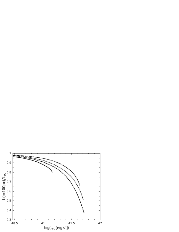
Figure 5: The fraction of inserted energy retained by stationary winds as a function of the star cluster luminosity, for $\beta$ = 0, 1, 1.5 and 2. (solid, long dashed, short dashed and dash dotted lines, respectively)

5.3.1 The Critical Line - semi-analytical solutions and 1D hydrodynamic simulations

For larger mass clusters or larger mechanical luminosities, one would soon reach the point above which a stationary wind solution does not exist. Physically this means that the hot gas inside the cluster is so dense that the energy deposition by massive stars cannot balance the loses due to expansion and radiative cooling and a large fraction of the gas inevitably cools down. As soon as the temperature drops to several times $10^{5}$ K radiative cooling becomes extremely fast due to free-bound and bound-bound transitions and some regions cool down very quickly to $\sim 10^{4}$ K (we do not allow the gas to cool below this temperature assuming that there are enough UV photons to maintain the gas warm and ionized). Consequently, these warm regions are compressed into dense clumps by the surrounding hot gas where the pressure is initially approximately three orders of magnitude larger.

For a given combination of cluster parameters $\beta$, $R_{c}$ and $R_{SC}$, there is a critical luminosity, $L_{crit}$, separating the region of stationary winds from the region where thermal instabilities occur within the cluster volume what leads to clump formation and to non-stationary outflows. The critical luminosity can be determined either by the semi-analytical code by searching for the $L_{SC}$ above which the solution of equations (12)-(14) does not exist, or by 1D hydrodynamic simulations.

In the case of semi-analytical calculations, we distinguish the two following situations: a) Clusters with $\beta=0$, clusters with $\beta>\beta_{crit}$, and compact clusters with $\beta\leq\beta_{crit}$ (e.g. for $\beta=1$ and $R_{SC}/R_{c}\lessapprox 8$ and $R_{SC}/R_{c}\lessapprox 4.3$ for $\beta=0.5$ ). For these clusters the criterion discussed in Tenorio-Tagle et al. (2007) for the homogeneous case, was used. i.e. the transition to the thermally unstable solutions occurs soon after the central temperature $T_{pm}$ drops to the value which corresponds to the maximum of the central pressure. This temperature is irrespective of the values of $\beta$, $R_{c}$ and $R_{SC}$ and depends only on $V_{A\infty}$ and $Z$. $T_{pm}$ can be calculated by solving the equation:

$$1-\frac{q_{m0}\mu_{a}T_{pm}}{2\mu_{i}n_{0}^{2}\Lambda(T_{pm},Z)}\left[\frac{c_{0}^{2}}{(\gamma-1)T_{pm}}+\frac{n_{0}^{2}}{q_{m0}}\frac{{\rm d}\Lambda(T_{pm},Z)}{{\rm d}T_{pm}}\right]=0,$$ (27)

which is equivalent to equation (7) of Silich et al. (2009) with the heating efficiency, $\eta=1$.
All these cases have in common the fact that $R_{sg}$ remains at its adiabatic position. b) More extended clusters with $\beta\leq\beta_{crit}$ (e.g. for $\beta$ = 1 with $R_{SC}/R_{c}\gtrapprox 8$ and for $\beta=0.5$ and $R_{SC}/R_{c}\gtrapprox 4.3$). In these cases, strong radiative cooling forces $R_{son}$ to detach from its adiabatic position, moving towards the center as one considers more massive clusters. Thus, the run of the hydrodynamical variables changes qualitatively, promoting the onset of thermal instabilities. Therefore, $L_{crit}$ is defined as the value for which $R_{son}$ begins to detach from its adiabatic position. The two semi-analytical criteria have been combined to define a unique semi-analytical curve for $L_{crit}$ (see Figure 6).

In the case of 1D hydrodynamical simulations, we vary $L_{SC}$ and use the bisection method to search for the largest $L_{SC}$ for which no zones with temperature smaller than $10^{5}$ K appear inside of the cluster or in the case of Models III and IV in the region $r<1.1R_{sg,adia}$, where $R_{sg,adia}$ is the singular point for clusters in the adiabatic regime with a given $\beta$ (calculated using equation (26)).

Figure 6 compares the results of the semi-analytical calculations with numerical results for different $\beta$ values. Since $L_{crit}$ is directly proportional to the size of the cluster, as shown by W08 for clusters with the top-hat profiles, the critical luminosity $L_{crit}$ is normalized to the star cluster core radius $L_{crit}/R_{c}$ and is presented as a function of the normalized star cluster radius $R_{SC}/R_{c}$ (left panel), or normalized star cluster half-mass radius $R_{hm}/R_{c}$ (right panel). In the case of top-hat profiles, with $\beta=0$, we normalized to $R_{c}=1$ pc. This makes the top-hat cluster radius or top-hat cluster half-mass radius dimensionless and comparable to other profiles with different values of $\beta$. There is a good correspondence between the results of semi-analytical and 1D hydrodynamical simulations.

Figure 6: $L_{crit}/R_{c}$ as a function of $R_{SC}/R_{c}$ (left panel) and $R_{hm}/R_{c}$ (right panel) for $\beta=0$ (solid line), $\beta=1$ (dashed line), $\beta=1.5$ (dotted line) and $\beta=2$ (dash - dotted line). Lines correspond to the semi-analytic results and open circles give the results of the 1D hydro-simulations.

At low values of $R_{SC}/R_{c}$, where $R_{SC}<R_{c}$, all the curves follow the critical luminosity of the top-hat profile ($\beta=0$). At somewhat larger values of $R_{SC}/R_{c}$, critical luminosities for models with $\beta>0$ deviate from the top-hat line towards higher luminosities. This is because their steeper stellar densities lead to the fastly growing wind velocities and there is less time for cooling and clump formation. Therefore, the cluster wind density and hence the luminosity must be larger to reach the thermally unstable regime. At even higher values, $R_{SC}/R_{c}>10$, the critical lines of models with $\beta\geq 1.5$ deviate from the top-hat line towards smaller luminosities reaching a constant value as $R_{SC}\rightarrow\infty$. This is because the denser central regions of these clusters undergoing rapid radiative cooling are not influenced by a further increase of $R_{SC}$. Critical luminosity curves for models with $0<\beta<1.5$ deviate at large $R_{SC}/R_{c}$ from the top-hat critical line, however since the mass contribution of their peripheral parts is never negligible, they have even for $R_{SC}/R_{c}\rightarrow\infty$ some non-zero slope of the $L_{crit}/R_{c}$ vs $R_{SC}/R_{c}$ line depending on the value of $\beta$.

The $L_{crit}/R_{c}$ vs $R_{hm}/R_{c}$ profiles are shown in the right panel of Figure 6. They are similar to $L_{crit}/R_{c}$ vs $R_{SC}/R_{c}$ profiles. The difference appears at the high $R_{hm}/R_{c}$ values: for $\beta\geq 1.5$ the $R_{hm}/R_{c}$ can not grow to infinity. It has a finite value depending on $\beta$. For $\beta$ = 2 it is about 2.26 and for $\beta$ = 1.5 it is about 36.84.

6 Summary

We have developed a model for the winds driven by stellar clusters with a generalized Schuster stellar density distribution. Two methods: a semi-analytic solution and 1D hydrodynamical simulations have been thoroughly discussed and shown in excellent agreement for clusters whose mechanical luminosities do not exceed the critical value, $L_{crit}$.

The semi-analytic solution cannot be applied for clusters with $L_{SC}>L_{crit}$ as in this case radiative cooling is extremely fast and the solution becomes thermally unstable. Nevertheless, assuming spherically symmetric star clusters, we have inferred the properties of stationary star cluster winds. For example, we have shown that in the adiabatic case, when radiative cooling is excluded, the position of the sonic point $R_{son}$, where the wind speed reaches the local sound speed, is given by the steepness of the stellar density distribution, if the singular point $R_{sg}$ of the equation (12) for the radial gradient of the wind speed is inside of the cluster: $R_{sg}=R_{son}<R_{SC}$. $R_{sg}$ is larger in clusters with flatter stellar density distributions (smaller $\beta$) and goes to infinity for $\beta\leq\beta_{crit}$, where $\beta_{crit}=9/8$. This implies that inside clusters with flat stellar density distributions the flow is always subsonic and the transition to the supersonic flow occurs at the star cluster surface, whereas in clusters with steeper density distributions the transition to the supersonic regime may occur either inside of the cluster, or at its surface, depending on whether the value of the cut-off radius $R_{SC}$ is larger or smaller than that of the singular point $R_{sg}$.

The position of the sonic point either inside the cluster or on its surface leads to two kinds of very different winds: in the first case the wind velocity increases gradually from the cluster center, while in the shallow cases there is a very slow subsonic wind inside the cluster and a strong wind acceleration to supersonic speed just at the cluster surface.

As one considers more massive clusters, the wind density increases implying a growing influence of radiative cooling: a fraction of the wind mechanical energy is lost and the wind temperature, velocity and sound speed decrease. The most energetic stationary winds exist for clusters with moderate steepnesses ($\beta=1-1.5$) although a large fraction of this energy is lost by radiation. For less or more steep stellar density profiles the wind becomes non-stationary at lower mechanical luminosities. The steepness of the stellar density profile also regulates the fraction of energy that is radiated away. Steeper stellar distributions lead to smaller sizes of the high density strongly radiative central regions with high wind speeds: there is less time for cooling of winds in clusters with steep stellar density profiles.

The dependence on the star cluster parameters, was explored. The normalized critical energy, $L_{crit}/R_{c}$, was calculated as a function of the normalized star cluster radius, $R_{SC}/R_{c}$ , and also as a function of the normalized star cluster half-mass radius, $R_{hm}/R_{c}$, and is plotted in Figure 6. One can compare target cluster parameters with these critical lines in order to find if radiative cooling may affect the star cluster driven flow significantly. The position of the normalized critical line $L_{crit}/R_{c}$ separates stationary winds from non-stationary winds in which frequent thermal instabilities in the deposited matter lead to the rapid condensation of unstable parcels of gas forming cold cloudlets immersed in the pervasive hot matter.

Clusters with a decreasing stellar density ($\beta>0$) and $R_{SC}<10\times R_{c}$ have $L_{crit}/R_{c}$ at higher values compared to the top-hat ($\beta=0$) stellar density profiles. If $R_{SC}>10\times R_{c}$, in clusters with a steep stellar density distribution ($\beta\geq 1.5$), the critical luminosity $L_{crit}/R_{c}$ approaches a constant value because the central cooling regions are only marginally influenced by increasing $R_{SC}/R_{c}$.

The non-stationary winds formed in high mass clusters with the total luminosity above the critical value $L_{crit}$ will be explored using 3D hydrodynamical simulations in a forthcoming communication. We shall also investigate if there are clusters formed with a mass near the critical luminosity $L_{crit}$. The very compact MW cluster Arches is a candidate. Also some compact clusters in the LMC or in M82 and the Antennae galaxies may be close or above the critical line suffering from strong internal cooling.

References

- Book et al. (2009) Book, L. G., Chu, Y.-H., Gruendl, R. A., & Fukui, Y. 2009, AJ, 137, 3599
- Cantó et al. (2000) Cantó, J., Raga, A. C., & Rodríguez, L. F. 2000, ApJ, 536, 896
- Chevalier & Clegg (1985) Chevalier, R. A. & Clegg, A. W. 1985, ApJ, 317, 44
- Dawson et al. (2013) Dawson, J. R., McClure-Griffiths, N. M., Wong, T., et al. 2013, ApJ, 763, 56
- Dib et al. (2007) Dib, S., Kim, J., & Shadmehri, M. 2007, MNRAS, 381, L40
- Elson et al. (1987) Elson, R. A. W., Fall, S. M., & Freeman, K. C. 1987, ApJ, 323, 54
- Fryxell et al. (2000) Fryxell, B., Olson, K., Ricker, P., et al. 2000, ApJS, 131, 273
- Ji et al. (2006) Ji, L., Wang, Q. D., & Kwan, J. 2006, MNRAS, 372, 497
- Johnson & Axford (1971) Johnson, H. E. & Axford, W. I. 1971, ApJ, 165, 381
- King (1962) King, I. 1962, AJ, 67, 471
- King (1966) King, I. R. 1966, AJ, 71, 64
- Mengel et al. (2002) Mengel, S., Lehnert, M. D., Thatte, N., & Genzel, R. 2002, A&A, 383, 137
- Ninkovic (1998) Ninkovic, S. 1998, Serbian Astronomical Journal, 158, 15
- Oey et al. (2005) Oey, M. S., Watson, A. M., Kern, K., & Walth, G. L. 2005, AJ, 129, 393
- Plewa (1995) Plewa, T. 1995, MNRAS, 275, 143
- Portegies Zwart et al. (2010) Portegies Zwart, S. F., McMillan, S. L. W., & Gieles, M. 2010, ARA&A, 48, 431
- Raymond et al. (1976) Raymond, J. C., Cox, D. P., & Smith, B. W. 1976, ApJ, 204, 290
- Rodríguez-González et al. (2007) Rodríguez-González, A., Cantó, J., Esquivel, A. & Velázquez, P. F. 2007, MNRAS, 380, 1198
- Sarazin & White (1987) Sarazin, C. L. & White, III, R. E. 1987, ApJ, 320, 32
- Silich et al. (2011) Silich, S., Bisnovatyi-Kogan, G., Tenorio-Tagle, G., & Martínez-González, S. 2011, ApJ, 743, 120
- Silich et al. (2004) Silich, S., Tenorio-Tagle, G., & Rodríguez-González, A. 2004, ApJ, 610, 226
- Silich et al. (2009) Silich, S., Tenorio-Tagle, G., Torres-Campos, A., et al. 2009, ApJ, 700, 931
- Tenorio-Tagle & Muñoz-Tuñón (1998) Tenorio-Tagle, G. & Muñoz-Tuñón, C. 1998, MNRAS, 293, 299
- Tenorio-Tagle et al. (2003) Tenorio-Tagle, G., Silich, S., & Muñoz-Tuñón, C. 2003, ApJ, 597, 279
- Tenorio-Tagle et al. (2010) Tenorio-Tagle, G., Wünsch, R., Silich, S., Muñoz-Tuñón, C., & Palouš, J. 2010, ApJ, 708, 1621
- Tenorio-Tagle et al. (2007) Tenorio-Tagle, G., Wünsch, R., Silich, S., & Palouš, J. 2007, ApJ, 658, 1196
- Veltmann (1979) Veltmann, U. I. K. 1979, AZh, 56, 976
- Wang et al. (2010) Wang, J., Feigelson, E. D., Townsley, L. K., et al. 2010, ApJ, 716, 474
- Whitmore et al. (1999) Whitmore, B. C., Zhang, Q., Leitherer, C., et al. 1999, AJ, 118, 1551
- Whitworth & Ward-Thompson (2001) Whitworth, A. P. & Ward-Thompson, D. 2001, ApJ, 547, 317
- Wünsch et al. (2007) Wünsch, R., Silich, S., Palouš, J., & Tenorio-Tagle, G. 2007, A&A, 471, 579
- Wünsch et al. (2011) Wünsch, R., Silich, S., Palouš, J., Tenorio-Tagle, G., & Muñoz-Tuñón, C. 2011, ApJ, 740, 75
- Wünsch et al. (2013) Wünsch, R., Tenorio-Tagle, G., Ehlerova, S., et al. 2013, in preparation, 999, 000
- Wünsch et al. (2008) Wünsch, R., Tenorio-Tagle, G., Palouš, J., & Silich, S. 2008, ApJ, 683, 683