Likelihood Geometry

Abstract

We study the critical points of monomial functions over an algebraic subset of the probability simplex. The number of critical points on the Zariski closure is a topological invariant of that embedded projective variety, known as its maximum likelihood degree. We present an introduction to this theory and its statistical motivations. Many favorite objects from combinatorial algebraic geometry are featured: toric varieties, $A$-discriminants, hyperplane arrangements, Grassmannians, and determinantal varieties. Several new results are included, especially on the likelihood correspondence and its bidegree. This article represents the lectures given by the second author at the CIME-CIRM course on Combinatorial Algebraic Geometry at Levico Terme in June 2013.

Introduction

Maximum likelihood estimation (MLE) is a fundamental computational problem in statistics, and it has recently been studied with some success from the perspective of algebraic geometry. In these notes we give an introduction to the geometry behind MLE for algebraic statistical models for discrete data. As is customary in algebraic statistics [15], we shall identify such models with certain algebraic subvarieties of high-dimensional complex projective spaces.

The article is organized into four sections. The first three sections correspond to the three lectures given at Levico Terme. The last section will contain proofs of new results.

In Section 1, we start out with plane curves, and we explain how to identify the relevant punctured Riemann surfaces. We next present the definitions and basic results for likelihood geometry in $\mathbb{P}^{n}$. Theorems 1.6 and 1.7 are concerned with the likelihood correspondence, the sheaf of differential $1$-forms with logarithmic poles, and the topological Euler characteristic. The ML degree of generic complete intersections is given in Theorem 1.10. Theorem 1.15 shows that the likelihood fibration behaves well over strictly positive data. Examples of Grassmannians and Segre varieties are discussed in detail. Our treatment of linear spaces in Theorem 1.20 will appeal to readers interested in matroids and hyperplane arrangements.

Section 2 begins leisurely, with the question Does watching soccer on TV cause hair loss? [34]. This leads us to conditional independence and low rank matrices. We study likelihood geometry of determinantal varieties, culminating in the duality theorem of Draisma and Rodriguez [14]. The ML degrees in Theorems 2.2 and 2.6 were computed using the software Bertini [6], underscoring the benefits of using numerical algebraic geometry for MLE. After a discussion of mixture models, highlighting the distinction between rank and nonnegative rank, we end Section 2 with a review of recent results in [1] on tensors of nonnegative rank $2$.

Section 3 starts out with toric models [37, §1.22] and geometric programming [9, §4.5]. Theorem 3.2 identifies the ML degree of a toric variety with the Euler characteristic of the complement of a hypersurface in a torus. Theorem 3.7 furnishes the ML degree of a variety parametrized by generic polynomials. Theorem 3.10 characterizes varieties of ML degree $1$ and it reveals a beautiful connection to the $A$-discriminant of [19]. We introduce the ML bidegree and the sectional ML degree of an arbitrary projective variety in $\mathbb{P}^{n}$, and we explain how these two are related. Section 3 ends with a study of the operations of intersection, projection, and restriction in likelihood geometry. This concerns the algebro-geometric meaning of the distinction between sampling zeros and structural zeros in statistical modeling.

In Section 4 we offer precise definitions and technical explanations of more advanced concepts from algebraic geometry, including logarithmic differential forms, Chern-Schwartz-MacPherson classes, and schön very affine varieties. This enables us to present complete proofs of various results, both old and new, that are stated in the earlier sections.

We close the introduction with a disclaimer regarding our overly ambitious title. There are many important topics in the statistical study of likelihood inference that should belong to “Likelihood Geometry” but are not covered in this article. Such topics include Watanabe’s theory of singular Bayesian integrals [45], differential geometry of likelihood in information geometry [5], and real algebraic geometry of Gaussian models [43]. We regret not being able to talk about these topics and many others. Our presentation here is restricted to the setting of [15, §2.2], namely statistical models for discrete data viewed as projective varieties in $\mathbb{P}^{n}$.

1 First Lecture

Let us begin our discussion with likelihood on algebraic curves in the complex projective plane $\mathbb{P}^{2}$. We fix a system of homogeneous coordinates $p_{0},p_{1},p_{2}$ on $\mathbb{P}^{2}$. The set of real points in $\mathbb{P}^{2}$ with ${\rm sign}(p_{0})={\rm sign}(p_{1})={\rm sign}(p_{2})$ is identified with the open triangle

$$\Delta_{2}\,\,=\,\,\bigl{\{}\,(p_{0},p_{1},p_{2})\in\mathbb{R}^{3}\,:\,p_{0},p_{1},p_{2}>0\,\,\,\hbox{and}\,\,\,p_{0}+p_{1}+p_{2}=1\,\bigr{\}}.$$

Given three positive integers $u_{0},u_{1},u_{2}$, the corresponding likelihood function is

$$\ell_{u_{0},u_{1},u_{2}}(p_{0},p_{1},p_{2})\,\,=\,\,\frac{p_{0}^{u_{0}}p_{1}^{u_{1}}p_{2}^{u_{2}}}{(p_{0}+p_{1}+p_{2})^{u_{0}+u_{1}+u_{2}}}.$$

This defines a rational function on $\mathbb{P}^{2}$, and it restricts to a regular function on $\mathbb{P}^{2}\backslash\mathcal{H}$, where

$$\mathcal{H}\,\,=\,\bigl{\{}\,(p_{0}:p_{1}:p_{2})\in\mathbb{P}^{2}\,:\,p_{0}p_{1}p_{2}(p_{0}+p_{1}+p_{2})=0\,\bigr{\}}$$

is our arrangement of four distinguished lines. The likelihood function $\ell_{u_{0},u_{1},u_{2}}$ is positive on the triangle $\Delta_{2}$, it is zero on the boundary of $\Delta_{2}$, and it attains its maximum at the point

$$(\hat{p}_{0},\hat{p}_{1},\hat{p}_{2})\,\,=\,\,\frac{1}{u_{0}+u_{1}+u_{2}}(u_{0},u_{1},u_{2}).$$ (1.1)

The corresponding point $(\hat{p}_{0}:\hat{p}_{1}:\hat{p}_{2})$ is the only critical point of the function $\ell_{u_{0},u_{1},u_{2}}$ on the four-dimensional real manifold $\mathbb{P}^{2}\backslash\mathcal{H}$. To see this, we consider the logarithmic derivative

$${\rm dlog}(\ell_{u_{0},u_{1},u_{2}})\,\,=\,\,\biggl{(}\frac{u_{0}}{p_{0}}-\frac{u_{0}+u_{1}+u_{2}}{p_{0}+p_{1}+p_{2}}\,,\,\,\frac{u_{1}}{p_{1}}-\frac{u_{0}+u_{1}+u_{2}}{p_{0}+p_{1}+p_{2}}\,,\,\,\frac{u_{2}}{p_{2}}-\frac{u_{0}+u_{1}+u_{2}}{p_{0}+p_{1}+p_{2}}\biggr{)}.$$

We note that this equals $(0,0,0)$ if and only if $(p_{0}:p_{1}:p_{2})$ is the point $(\hat{p}_{0}:\hat{p}_{1}:\hat{p}_{2})$ in (1.1).

Let $X$ be a smooth curve in $\mathbb{P}^{2}$ defined by a homogeneous polynomial $f(p_{0},p_{1},p_{2})$. This curve plays the role of a statistical model, and our task is to maximize the likelihood function $\ell_{u_{0},u_{1},u_{2}}$ over its set $X\cap\Delta_{2}$ of positive real points. To compute that maximum algebraically, we examine the set of all critical points of $\ell_{u_{0},u_{1},u_{2}}$ on the complex curve $X\backslash\mathcal{H}$. That set of critical points is the likelihood locus. Using Lagrange Multipliers from Calculus, we see that it consists of all points of $X\backslash\mathcal{H}$ such that ${\rm dlog}(\ell_{u_{0},u_{1},u_{2}})$ lies in the plane spanned by ${\rm d}f$ and $(1,1,1)$ in $\mathbb{C}^{3}$. Thus, our task is to study the solutions in $\mathbb{P}^{2}\backslash\mathcal{H}$ of the equations

$$f(p_{0},p_{1},p_{2})\,=\,0\qquad\hbox{and}\qquad{\rm det}\begin{pmatrix}1&1&1\vskip 3.0pt plus 1.0pt minus 1.0pt\\ \frac{u_{0}}{p_{0}}&\frac{u_{1}}{p_{1}}&\frac{u_{2}}{p_{2}}\vskip 6.0pt plus 2.0pt minus 2.0pt\\ \frac{\partial f}{\partial p_{0}}&\frac{\partial f}{\partial p_{1}}&\frac{\partial f}{\partial p_{2}}\end{pmatrix}\,=\,\,0.$$ (1.2)

Suppose that $X$ has degree $d$. Then, after clearing denominators, the second equation has degree $d+1$. By Bézout’s Theorem, we expect the likelihood locus to consist of $d(d+1)$ points in $\mathbb{P}^{2}\backslash\mathcal{H}$. This is indeed what happens when $f$ is a generic polynomial of degree $d$.

We define the maximum likelihood degree (or ML degree) of our curve $X$ to be the cardinality of the likelihood locus for generic choices of $u_{0},u_{1},u_{2}$. Thus a general plane curve of degree $d$ has ML degree $d(d+1)$. However, for special curves, the ML degree can be smaller.

Theorem 1.1.

Let $X$ be a smooth curve of degree $d$ in $\mathbb{P}^{2}$, and $a=\#(X\cap\mathcal{H})$ the number of its points on the distinguished arrangement. Then the ML degree of $X$ equals $d^{2}-3d+a$.

This is a very special case of Theorem 1.7 which identifies the ML degree with the signed Euler characteristic of $X\backslash\mathcal{H}$. For a general curve of degree $d$ in $\mathbb{P}^{2}$, we have $a=4d$, and so $d^{2}-3d+a=d(d+1)$ as predicted. However, the number $a$ of points in $X\cap\mathcal{H}$ can drop:

Example 1.2.

Consider the case $d=1$ of lines. A generic line has ML degree $2$. The line $X=V(p_{0}+cp_{1})$ has ML degree $1$ provided $c\not\in\{0,1\}$. The special line $X=V(p_{0}+p_{1})$ has ML degree $0$: (1.2) has no solutions on $X\backslash\mathcal{H}$ unless $u_{0}+u_{1}=0$. In the three cases, $X\backslash\mathcal{H}$ is the Riemann sphere $\mathbb{P}^{1}$ with four, three, or two points removed. $\diamondsuit$

Example 1.3.

Consider the case $d=2$ of quadrics. A general quadric has ML degree $6$. The Hardy-Weinberg curve, which plays a fundamental role in population genetics, is given by

$$f(p_{0},p_{1},p_{2})\,\,=\,\,{\rm det}\begin{pmatrix}2p_{0}&p_{1}\\ p_{1}&2p_{2}\end{pmatrix}\,\,=\,\,4p_{0}p_{2}-p_{1}^{2}.$$

The curve has only three points on the distinguished arrangement:

$$X\cap\mathcal{H}\,\,=\,\,\bigl{\{}\,(1:0:0),\,(0:0:1),\,(1:-2:1)\,\bigr{\}}.$$

Hence the ML degree of the Hardy-Weinberg curve equals $1$. This means that the maximum likelihood estimate (MLE) is a rational function of the data. Explicitly, the MLE equals

$$(\hat{p}_{0},\hat{p}_{1},\hat{p}_{2})\,\,=\,\,\frac{1}{4(u_{0}+u_{1}+u_{2})^{2}}\bigl{(}\,(2u_{0}+u_{1})^{2}\,,\,2(2u_{0}+u_{1})(u_{1}+2u_{2})\,,\,(u_{1}+2u_{2})^{2}\,\bigr{)}.$$ (1.3)

In applications, the Hardy-Weinberg curve arises via its parametric representation

$$\begin{matrix}p_{0}(s)&=&s^{2}\\ p_{1}(s)&=&2s(1-s)\\ p_{2}(s)&=&(1-s)^{2}\end{matrix}$$ (1.4)

Here the parameter $s$ is the probability that a biased coin lands on tails. If we toss that same biased coin twice, then the above formulas represent the following probabilities:

$$\begin{matrix}p_{0}(s)&=&\hbox{ probability of 0 heads}\\ p_{1}(s)&=&\hbox{ probability of 1 head}\\ p_{2}(s)&=&\hbox{ probability of 2 heads}\\ \end{matrix}$$

Suppose now that the experiment of tossing the coin twice is repeated $N$ times. We record the following counts, where $N=u_{0}+u_{1}+u_{2}$ is the sample size of our repeated experiment:

$$\begin{matrix}u_{0}&=&\hbox{ number of times 0 heads were observed}\\ u_{1}&=&\hbox{ number of times 1 head was observed}\\ u_{2}&=&\hbox{ number of times 2 heads were observed}\end{matrix}\qquad\qquad$$

The MLE problem is to estimate the unknown parameter $s$ by maximizing

$$\ell_{u_{0},u_{1},u_{2}}\,\,=\,\,p_{0}(s)^{u_{0}}p_{1}(s)^{u_{1}}p_{2}(s)^{u_{2}}\,\,=\,\,2^{u_{1}}s^{2u_{0}+u_{1}}(1-s)^{u_{1}+2u_{2}}.$$

The unique solution to this optimization problem is

$$\hat{s}\quad=\quad\frac{2u_{0}+u_{1}}{2u_{0}+2u_{1}+2u_{2}}.$$

Substituting this expression into (1.4) gives the estimator $\bigl{(}p_{0}(\hat{s}),p_{1}(\hat{s}),p_{2}(\hat{s})\bigr{)}$ for the three probabilities in our model. The resulting rational function coincides with (1.3). $\diamondsuit$

The ML degree is also defined when the given curve $X\subset\mathbb{P}^{2}$ is not smooth, but it counts critical points of $\ell_{u}$ only in the regular locus of $X$. Here is an example to illustrate this.

Example 1.4.

A general cubic curve $X$ in $\mathbb{P}^{2}$ has ML degree $12$. Suppose now that $X$ is a cubic which meets $\mathcal{H}$ transversally but has one isolated singular point in $\mathbb{P}^{2}\backslash\mathcal{H}$. If the singular point is a node then the ML degree of $X$ is $10$, and if the singular point is a cusp then the ML degree of $X$ is $9$. The ML degrees are found by saturating the equations in (1.2) with respect to the homogenous ideal of the singular point. $\diamondsuit$

Moving beyond likelihood geometry in the plane, we shall introduce our objects in any dimension. We fix the complex projective space $\mathbb{P}^{n}$ with coordinates $p_{0},p_{1},\ldots,p_{n}$, representing probabilities. We summarize the observed data in a vector $u=(u_{0},u_{1},\ldots,u_{n})\in\mathbb{N}^{n+1}$, where $u_{i}$ is the number of samples in state $i$. The likelihood function on $\mathbb{P}^{n}$ given by $u$ equals

$$\ell_{u}\quad=\quad\frac{p_{0}^{u_{0}}p_{1}^{u_{1}}\cdots p_{n}^{u_{n}}}{(p_{0}+p_{1}+\cdots+p_{n})^{u_{0}+u_{1}+\cdots+u_{n}}}.$$

The unique critical point of this rational function on $\mathbb{P}^{n}$ is the data point itself:

$$(u_{0}:u_{1}:\cdots:u_{n}).$$

Moreover, this point is the global maximum of the likelihood function $\ell_{u}$ on the probability simplex $\Delta_{n}$. Throughout, we identify $\Delta_{n}$ with the set of all positive real points in $\mathbb{P}^{n}$.

The linear forms in $\ell_{u}$ define an arrangement $\mathcal{H}$ of $n+2$ distinguished hyperplanes in $\mathbb{P}^{n}$. The differential of the logarithm of the likelihood function is the vector of rational functions

$${\rm dlog}(\ell_{u})\,=\,\bigl{(}\frac{u_{0}}{p_{0}},\frac{u_{1}}{p_{1}},\ldots,\frac{u_{n}}{p_{n}}\bigr{)}-\frac{u_{+}}{p_{+}}\cdot(1,1,\ldots,1).$$ (1.5)

Here ${p_{+}}=\sum_{i=0}^{n}p_{i}$ and ${u_{+}}=\sum_{i=0}^{n}u_{i}$. The vector (1.5) represents a section of the sheaf of differential $1$-forms on $\mathbb{P}^{n}$ that have logarithmic singularities along $\mathcal{H}$. This sheaf is denoted

$$\Omega_{\mathbb{P}^{n}}^{1}({\rm log}(\mathcal{H})).$$

Our aim is to study the restriction of $\ell_{u}$ to a closed subvariety $X\subseteq\mathbb{P}^{n}$. We will assume that $X$ is defined over the real numbers, irreducible, and not contained in $\mathcal{H}$. Let $X_{\rm sing}$ denote the singular locus of $X$, and $\,X_{\rm reg}$ denote $X\backslash X_{\rm sing}$. When $X$ serves as a statistical model, the goal is to maximize the rational function $\ell_{u}$ on the semialgebraic set $X\cap\Delta_{n}$. To solve this problem algebraically, we determine all critical points of the log-likelihood function ${\rm log}(\ell_{u})$ on the complex variety $X$. Here we must exclude points that are singular or lie in $\mathcal{H}$.

Definition 1.5.

The maximum likelihood degree of $X$ is the number of complex critical points of the function $\ell_{u}$ on $X_{\rm reg}\backslash\mathcal{H}$, for generic data $u$. The likelihood correspondence $\mathcal{L}_{X}$ is the universal family of these critical points. To be precise, $\mathcal{L}_{X}$ is the closure in $\mathbb{P}^{n}\times\mathbb{P}^{n}$ of

$$\bigl{\{}(p,u)\,:\,p\in X_{\rm reg}\backslash\mathcal{H}\,\,\hbox{and}\,\,\,{\rm dlog}(\ell_{u})\,\,\hbox{vanishes at $p$}\bigr{\}}.$$

We sometimes write $\,\mathbb{P}^{n}_{p}\times\mathbb{P}^{n}_{u}\,$ for $\,\mathbb{P}^{n}\times\mathbb{P}^{n}\,$ to highlight that the first factor is the probability space, with coordinates $p$, while the second factor is the data space, with coordinates $u$. The first part of the following result appears in [25, §2]. A precursor was [23, Proposition 3].

Theorem 1.6.

The likelihood correspondence $\mathcal{L}_{X}$ of any irreducible subvariety $X$ in $\mathbb{P}^{n}_{p}$ is an irreducible variety of dimension $n$ in the product $\,\mathbb{P}^{n}_{p}\times\mathbb{P}^{n}_{u}$. The map ${\rm pr}_{1}:\mathcal{L}_{X}\rightarrow\mathbb{P}^{n}_{p}$ is a projective bundle over $X_{\rm reg}\backslash\mathcal{H}$, and the map ${\rm pr}_{2}:\mathcal{L}_{X}\rightarrow\mathbb{P}^{n}_{u}$ is generically finite-to-one.

See Section 4 for a proof. The degree of the map ${\rm pr}_{2}:\mathcal{L}_{X}\rightarrow\mathbb{P}^{n}_{u}$ to data space is the ML degree of $X$. This number has a topological interpretation as an Euler characteristic, provided suitable assumptions on $X$ are being made. The relationship between the homology of a manifold and critical points of a suitable function on it is the topic of Morse theory.

The study of ML degrees was started in [10, §2] by developing the connection to the sheaf $\,\Omega^{1}_{X}({\rm log}(\mathcal{H}))$ of differential $1$-forms on $X$ with logarithmic poles along $\mathcal{H}$. It was shown in [10, Theorem 20] that the ML degree of $X$ equals the signed topological Euler characteristic

$$(-1)^{\dim X}\cdot\chi(X\backslash\mathcal{H}),$$

provided $X$ is smooth and the intersection $\mathcal{H}\cap X$ defines a normal crossing divisor in $X\subseteq\mathbb{P}^{n}$. A major drawback of that early result was that the hypotheses are so restrictive that they essentially never hold for varieties $X$ that arise from statistical models used in practice. From a theoretical point view, this issue can be addressed by passing to a resolution of singularities. However, in spite of existing algorithms for resolution in characteristic zero, these algorithms do not scale to problems of the sizes of interest in algebraic statistics. Thus, whatever computations we wish to do should not be based on resolution of singularities.

The following result due to [25] gives the same topological interpretation of the ML degree. The hypotheses here are much more realistic and inclusive than those in [10, Theorem 20].

Theorem 1.7.

If the very affine variety $X\backslash\mathcal{H}$ is smooth of dimension $d$, then the ML degree of $X$ equals the signed topological Euler characteristic of $(-1)^{d}\cdot\chi(X\backslash\mathcal{H})$.

The term very affine variety refers to a closed subvariety of some algebraic torus $(\mathbb{C}^{*})^{m}$. Our ambient space $\mathbb{P}^{n}\backslash\mathcal{H}$ is a very affine variety because it has a closed embedding

$$\mathbb{P}^{n}\backslash\mathcal{H}\longrightarrow(\mathbb{C}^{*})^{n+1},\qquad(p_{0}:\cdots:p_{n})\longmapsto\big{(}\frac{p_{0}}{p_{+}},\ldots,\frac{p_{n}}{p_{+}}\big{)}.$$

The study of such varieties is foundational for tropical geometry. The special case when $X\backslash\mathcal{H}$ is a Riemann surface with $a$ punctures, arising from a curve in $\mathbb{P}^{2}$, was seen in Theorem 1.1. We remark that Theorem 1.7 can be deduced from works of Gabber-Loeser [18] and Franecki-Kapranov [16] on perverse sheaves on algebraic tori.

The smoothness hypothesis is essential for Theorem 1.7 to hold. If $X$ is singular then, generally, neither $X\backslash\mathcal{H}$ nor $X_{\rm reg}\backslash\mathcal{H}$ has its signed Euler characteristic equal to the ML degree of $X$. Varieties $X$ that demonstrate this are the two singular cubic curves in Example 1.4.

Conjecture 1.8.

For any projective variety $X\subseteq\mathbb{P}^{n}$ of dimension $d$, not contained in $\mathcal{H}$,

$$(-1)^{d}\cdot\chi(X\backslash\mathcal{H})\,\,\geq\,\,{\rm MLdegree}\,(X).$$

In particular, the signed topological Euler characteristic $(-1)^{d}\cdot\chi(X\backslash\mathcal{H})$ is nonnegative.

Analogous conjectures can be made in the slightly more general setting of [25]. In particular, we conjecture that the inequality

$$(-1)^{d}\cdot\chi(V)\,\geq\,0$$

holds for any closed $d$-dimensional subvariety $V\subseteq(\mathbb{C}^{*})^{m}$.

Remark 1.9.

We saw in Example 1.2 that the ML degree of a projective variety $X$ can be $0$. In all situations of statistical interest, the variety $X\subset\mathbb{P}^{n}$ intersects the open simplex $\Delta_{n}$ in a subset that is Zariski dense in $X$. If that intersection is smooth then ${\rm MLdegree}(X)\geq 1$. In fact, arguing as in [10, Proposition 11], it can be shown that for smooth $X$,

$${\rm MLdegree}\,(X)\,\,\geq\,\,\#(\text{bounded regions of $X_{\mathbb{R}}\backslash\mathcal{H}$}).$$

Here a bounded region is a connected component of the semialgebraic set $X_{\mathbb{R}}\backslash\mathcal{H}$ whose classical closure is disjoint from the distinguished hyperplane $V(p_{+})$ in $\mathbb{P}^{n}$.

If $X$ is singular then the number of bounded regions of $X_{\mathbb{R}}\backslash\mathcal{H}$ can exceed ${\rm MLdegree}\,(X)$. For instance, let $X\subset\mathbb{P}^{2}$ be the cuspidal cubic curve defined by

$$(p_{0}{+}p_{1}{+}p_{2})(7p_{0}{-}9p_{1}{-}2p_{2})^{2}=(3p_{0}{+}5p_{1}{+}4p_{2})^{3}.$$

The real part $X_{\mathbb{R}}\backslash\mathcal{H}$ consists of $8$ bounded and $2$ unbounded regions, but the ML degree of $X$ is $7$. The bounded region that contains the cusp $(13:17:-31)$ has no other critical points for $\ell_{u}$. $\diamondsuit$

In what follows we present instances that illustrate the computation of the ML degree. We begin with the case of generic complete intersections. Suppose that $X\subset\mathbb{P}^{n}$ is a complete intersection defined by $r$ generic homogeneous polynomials $g_{1},\ldots,g_{r}$ of degrees $d_{1},d_{2},\ldots,d_{r}$.

Theorem 1.10.

The ML degree of $X$ equals $Dd_{1}d_{2}\cdots d_{r}$, where

$$D\,\quad=\,\sum_{i_{1}+i_{2}+\cdots+i_{r}\leq n-r}\!\!\!\!\!d_{1}^{i_{1}}d_{2}^{i_{2}}\cdots d_{r}^{i_{r}}.$$ (1.6)

Proof.

By Bertini’s Theorem, the generic complete intersection $X$ is smooth in $\mathbb{P}^{n}$. All critical points of the likelihood function $\ell_{u}$ on $X$ lie in the dense open subset $X\backslash\mathcal{H}$. Consider the following $(r+2)\times(n+1)$-matrix with entries in the polynomial ring $\mathbb{R}[p_{0},p_{1},\ldots,p_{n}]$:

$$\begin{bmatrix}u\\ {\tilde{J}}(p)\end{bmatrix}\quad=\quad\begin{bmatrix}&u_{0}&u_{1}&\cdots&u_{n}\\ &p_{0}&p_{1}&\cdots&p_{n}\vskip 3.0pt plus 1.0pt minus 1.0pt\\ &p_{0}\frac{\partial g_{1}}{\partial p_{0}}&p_{1}\frac{\partial g_{1}}{\partial p_{1}}&\cdots&p_{n}\frac{\partial g_{1}}{\partial p_{n}}\vskip 6.0pt plus 2.0pt minus 2.0pt\\ &p_{0}\frac{\partial g_{2}}{\partial p_{0}}&p_{1}\frac{\partial g_{2}}{\partial p_{1}}&\cdots&p_{n}\frac{\partial g_{2}}{\partial p_{n}}\\ &\vdots&\vdots&\ddots&\vdots&\vskip 3.0pt plus 1.0pt minus 1.0pt\\ &p_{0}\frac{\partial g_{r}}{\partial p_{0}}&p_{1}\frac{\partial g_{r}}{\partial p_{1}}&\cdots&p_{n}\frac{\partial g_{r}}{\partial p_{n}}\end{bmatrix}.$$ (1.7)

Let $Y$ denote the determinantal variety in $\mathbb{P}^{n}$ given by the vanishing of its $(r+2)\times(r+2)$ minors. The codimension of $Y$ is at most $n-r$, which is a general upper bound for ideals of maximal minors, and hence the dimension of $Y$ is at least $r$. Our genericity assumptions ensure that the matrix $\tilde{J}(p)$ has maximal row rank $r+1$ for all $p\in X$. Hence a point $p\in X$ lies in $Y$ if and only if the vector $u$ is in the row span of $\tilde{J}(p)$. Moreover, by Theorem 1.6,

$$(X_{\rm reg}\backslash\mathcal{H})\,\cap\,Y\quad=\quad X\,\cap\,Y$$

is a finite subset of $\mathbb{P}^{n}$, and its cardinality is the desired ML degree of $X$.

Since $X$ has dimension $n-r$, we conclude that $Y$ has the maximum possible codimension, namely $n-r$, and that the intersection of $X$ with the determinantal variety $Y$ is proper. We note that $Y$ is Cohen-Macaulay, since $Y$ has maximal codimension $n-r$, and ideals of minors of generic matrices are Cohen-Macaulay. Bézout’s Theorem implies

$${\rm MLdegree}(X)\quad=\quad{\rm degree}(X)\cdot{\rm degree}(Y)\quad=\quad d_{1}\cdots d_{r}\cdot{\rm degree}(Y).$$

The degree of the determinantal variety $Y$ equals the degree of the determinantal variety given by generic forms of the same row degrees. By the Thom-Porteous-Giambelli formula, this degree is the complete homogeneous symmetric function of degree $\,{\rm codim}(Y)=n-r\,$ evaluated at the row degrees of the matrix. Here, the row degrees are $\,0,1,d_{1},\ldots,d_{r}$, and the value of that symmetric function is precisely $D$. We conclude that ${\rm degree}(Y)=D$. Hence the ML degree of the generic complete intersection $\,X=\mathcal{V}(g_{1},\ldots,g_{r})\,$ equals $\,D\cdot d_{1}d_{2}\cdots d_{n}$. ∎

Example 1.11 ($r=1$).

A generic hypersurface of degree $d$ in $\mathbb{P}^{n}$ has ML degree

$$d\cdot D\,\,=\,\,d+d^{2}+d^{3}+\cdots+d^{n}.$$

Example 1.12 ($r=2,n=3$).

A space curve that is the generic intersection of two surfaces of degree $d$ and $e$ in $\mathbb{P}^{3}$ has ML degree $\,de+d^{2}e+de^{2}$. $\diamondsuit$

Remark 1.13.

It was shown in [23, Theorem 5] that (1.6) is an upper bound for the ML degree of any variety $X$ of codimension $r$ that is defined by polynomials of degree $d_{1},\ldots,d_{r}$. In fact, the same is true under the weaker hypothesis that $X$ is cut out by polynomials of degrees $d_{1}\geq\cdots\geq d_{r}\geq d_{r+1}\geq\cdots\geq d_{s}$, so $X$ need not be a complete intersection. However, the hypothesis ${\rm codim}(X)=r$ is essential in order for ${\rm MLdegree}(X)\leq$ (1.6) to hold. That codimension hypothesis was forgotten when this upper bound was cited in [15, Theorem 2.2.6] and in [37, Theorem 3.31]. Hence these two book references are not correct as stated.

Here is a simple counterexample. Let $n=3$ and $d_{1}=d_{2}=d_{3}=2$. Then the bound (1.6) is the Bézout number $8$, and this is also the correct ML degree for a general complete intersection of three quadrics in $\mathbb{P}^{3}$. Now let $X$ be a general rational normal curve in $\mathbb{P}^{3}$. The curve $X$ is defined by three quadrics, namely, the $2\times 2$-minors of a $2\times 3$-matrix filled with general linear forms in $p_{0},p_{1},p_{2},p_{3}$. Since $X$ is a Riemann sphere with $15$ punctures, Theorem 1.7 tells us that ${\rm MLdegree}(X)=13$, and this exceeds the bound of $8$. $\diamondsuit$

We now come to a variety that is ubiquitous in statistics, namely the model of independence for two binary random variables [15, §1.1]. This model is represented by Segre’s quadric surface $X$ in $\mathbb{P}^{3}$. By this we mean the surface defined by the $2\times 2$-determinant:

$$X\,=\,V(p_{00}p_{11}-p_{01}p_{10})\,\,\subset\,\,\mathbb{P}^{3}.$$

The surface $X$ is isomorphic to $\mathbb{P}^{1}\times\mathbb{P}^{1}$, so it is smooth, and we can apply Theorem 1.7 to find the ML degree. In other words, we seek to determine the Euler characteristic of the open complex surface $\,X\backslash\mathcal{H}\,$ where

$$\mathcal{H}=\bigl{\{}\,p\in\mathbb{P}^{3}:p_{00}p_{01}p_{10}p_{11}(p_{00}{+}p_{01}{+}p_{10}{+}p_{11})=0\bigr{\}}.$$

To this end, we write $X=\mathbb{P}^{1}\times\mathbb{P}^{1}$ with coordinates $\bigl{(}(x_{0}:x_{1}),(y_{0}:y_{1})\bigr{)}$. Our surface is parametrized by $p_{ij}=x_{i}y_{j}$, and hence

$$\begin{matrix}X\backslash\mathcal{H}&=&\big{(}\mathbb{P}^{1}\times\mathbb{P}^{1}\big{)}\backslash\big{\{}x_{0}x_{1}y_{0}y_{1}(x_{0}+x_{1})(y_{0}+y_{1})=0\big{\}}\qquad\qquad\vskip 3.0pt plus 1.0pt minus 1.0pt\\ &=&\big{(}\mathbb{P}^{1}\backslash\{x_{0}x_{1}(x_{0}+x_{1})=0\}\big{)}\,\times\,\big{(}\mathbb{P}^{1}\backslash\{y_{0}y_{1}(y_{0}+y_{1})=0\}\big{)}\vskip 3.0pt plus 1.0pt minus 1.0pt\\ &=&\big{(}\hbox{$2$-sphere}\backslash\{\hbox{three points}\}\big{)}\,\times\,\big{(}\hbox{$2$-sphere}\backslash\{\hbox{three points}\}\big{)}.\end{matrix}$$

Since the Euler characteristic is additive and multiplicative,

$$\chi(X\backslash\mathcal{H})\,\,=\,\,(-1)\cdot(-1)\,\,=\,\,1.$$

This means that the map $u\mapsto\hat{p}$ from the data to the MLE is a rational function in each coordinate. The following “word problem for freshmen” is aimed at finding that function.

Example 1.14.

Do this exercise: A biologist friend of yours wishes to test whether two binary random variables are independent. She collects data and records the matrix of counts

$$\,u\,\,=\,\,\begin{pmatrix}u_{00}&u_{01}\\ u_{10}&u_{11}\end{pmatrix}.$$

How to ascertain whether $u$ lies close to the independence model

$$\qquad X\,\,=\,\,V(p_{00}p_{11}-p_{01}p_{10})\,?$$

A statistician who recently started working in her lab explains that, as the first step in the analysis of her data, the biologist should calculate the maximum likelihood estimate (MLE)

$$\hat{p}\,=\,\begin{pmatrix}\hat{p}_{00}&\hat{p}_{01}\\ \hat{p}_{10}&\hat{p}_{11}\end{pmatrix}.$$

Can you help your friend by supplying the formula for $\hat{p}$ as a rational function in $u$?

The solution to this word problem is as follows. The MLE is the rank $1$ matrix

$$\hat{p}\,=\,\frac{1}{(u_{++})^{2}}\begin{pmatrix}u_{0+}\\ u_{1+}\end{pmatrix}\cdot\begin{pmatrix}u_{+0}&u_{+1}\end{pmatrix}.$$ (1.8)

We illustrate the concepts introduced above by deriving this well-known formula. The likelihood correspondence $\mathcal{L}_{X}$ of $\,X=V(p_{00}p_{11}-p_{01}p_{10})\,$ is the subvariety of $X\times\mathbb{P}^{3}$ defined by

$$U\cdot(p_{00},p_{01},p_{10},p_{11})^{T}\,\,=\,\,0,$$ (1.9)

where $U$ is the matrix

$$U\,\,=\,\,\begin{pmatrix}0&-u_{10}-u_{11}&0&u_{00}+u_{01}\\ u_{11}+u_{01}&-u_{00}-u_{10}&0&0\\ u_{11}+u_{10}&0&-u_{01}-u_{00}&0\\ 0&0&-u_{01}-u_{11}&u_{00}+u_{10}\end{pmatrix}.$$

We urge the reader to derive (1.9) from Definition 1.5 using a computer algebra system.

Note that the determinant of $U$ vanishes identically. In fact, for generic $u_{ij}$, the matrix $U$ has rank $3$, so its kernel is spanned by a single vector. The coordinates of that vector are given by Cramer’s rule, and we find them to be equal to the rational functions in (1.8).

The locus where the function $u\mapsto\hat{p}$ is undefined consists of those $u$ where the matrix rank of $U$ drops below $3$. A computation shows that the rank of $U$ drops to $2$ on the variety

$$V(u_{00}+u_{10},u_{01}+u_{11})\,\cup\,V(u_{00}+u_{01},u_{10}+u_{11}),$$

and it drops to $0$ on the point $\,V(u_{00}+u_{01},u_{10}+u_{11},u_{01}+u_{11})$. In particular, the likelihood function $\ell_{u}$ given by that point $u$ has infinitely many critical points in the quadric $X$. $\diamondsuit$

We note that all coefficients of the linear forms that define the exceptional loci in $\mathbb{P}^{3}_{u}$ for the independence model are positive. This means that data points $u$ with all coordinates positive can never be exceptional. We will prove in Section 4 that this usually holds. Let ${\rm pr}_{1}:\mathcal{L}_{X}\to\mathbb{P}^{n}_{p}$ and ${\rm pr}_{2}:\mathcal{L}_{X}\to\mathbb{P}^{n}_{u}$ be the projections from the likelihood correspondence to $p$-space and $u$-space respectively. We are interested in the fibers of ${\rm pr}_{2}$ over positive points $u$.

Theorem 1.15.

Let $u\in\mathbb{R}^{n+1}_{>0}$, and let $X\subset\mathbb{P}^{n}$ be an irreducible variety such that no singular points of any intersection $X\cap\{p_{i}=0\}$ lies in the hyperplane at infinity $\{p_{+}=0\}$. Then

1. the likelihood function $\ell_{u}$ on $X$ has only finitely many critical points in $X_{\rm reg}\backslash\mathcal{H}$;

2. if the fiber ${\rm pr}_{2}^{-1}(u)$ is contained in $X_{\rm reg}$, then its length equals the ML degree of $X$.

The hypothesis concerning “no singular point” will be satisfied for essentially all statistical models of interest. Here is an example which shows that this hypothesis is necessary.

Example 1.16.

We consider the smooth cubic curve $X$ in $\mathbb{P}^{2}$ that is defined by

$$f\,\,\,=\,\,\,(p_{0}+p_{1}+p_{2})^{3}\,+\,p_{0}p_{1}p_{2}.$$

The ML degree of the curve $X$ is $3$. Each intersection $X\cap\{p_{i}=0\}$ is a triple point that lies on the line at infinity $\{p_{+}=0\}$. The fiber ${\rm pr}_{2}^{-1}(u)$ of the likelihood fibration over the positive point $u=(1:1:1)$ is the entire curve $X$. $\diamondsuit$

If $u$ is not positive in Theorem 1.15, then the fiber of ${\rm pr}_{2}$ over $u$ may have positive dimension. We saw an instance of this at the end of Example 1.14. Such resonance loci have been studied extensively when $X$ is a linear subspace of $\mathbb{P}^{n}$. See [11] and references therein.

The following cautionary example shows that the length of the scheme-theoretic fiber of $\mathcal{L}_{X}\to\mathbb{P}^{n}_{u}$ over special points $u$ in the open simplex $\Delta_{n}$ may exceed the ML degree of $X$.

Example 1.17.

Let $X$ be the curve in $\mathbb{P}^{2}$ defined by the ternary cubic

$$f\,\,=\,\,p_{2}(p_{1}-p_{2})^{2}+(p_{0}-p_{2})^{3}.$$

This curve intersects $\mathcal{H}$ in $8$ points, has ML degree $5$, and has a cuspidal singularity at

$$P\,\,:=\,\,(1:1:1).$$

The prime ideal in $\mathbb{R}[p_{0},p_{1},p_{2},u_{0},u_{1},u_{2}]$ for the likelihood correspondence $\mathcal{L}_{X}$ is minimally generated by five polynomials, having degrees $(3,0),(2,2),(3,1),(3,1),(3,1)$. They are obtained by saturating the two equations in (1.2) with respect to $\,\langle p_{0}p_{2}\rangle\cap\langle p_{0}-p_{1},p_{2}-p_{1}\rangle$.

The scheme-theoretic fiber of ${\rm pr}_{1}$ over a general point of $X$ is a reduced line in the $u$-plane, while the fiber of ${\rm pr}_{1}$ over $P$ is the double line

$$L:=\big{\{}\,(u_{0}:u_{1}:u_{2})\in\mathbb{P}^{2}:(2u_{0}-u_{1}-u_{2})^{2}=0\,\big{\}}.$$

The reader is invited to verify the following assertions using a computer algebra system:

1. If $u$ is a general point of $\mathbb{P}^{2}_{u}$, then $\text{pr}_{2}^{-1}(u)$ consists of $5$ reduced points in $X_{\rm reg}\backslash\mathcal{H}$.

2. If $u$ is a general point on the line $L$, then the locus of critical points $\text{pr}_{2}^{-1}(u)$ consists of $4$ reduced points in $X_{\rm reg}\backslash\mathcal{H}$ and the reduced point $P$.

3. If $u$ is the point $(1:1:1)\in L$, then $\text{pr}_{2}^{-1}(u)$ is a zero-dimensional scheme of length $6$. This scheme consists of $3$ reduced points in $X_{\rm reg}\backslash\mathcal{H}$ and $P$ counted with multiplicity $3$.

In particular, the fiber in (c) is not algebraically equivalent to the general fiber (a). This example illustrates one of the difficulties classical geometers had to face when formulating the “principle of conservation of numbers”. See [17, Chapter 10] for a modern treatment. $\diamondsuit$

It is instructive to examine classical varieties from projective geometry from the likelihood perspective. For instance, we may study the Grassmannian in its Plücker embedding. Grassmannians are a nice test case because they are smooth, so that Theorem 1.7 applies.

Example 1.18.

Let $X=G(2,4)$ denote the Grassmannian of lines in $\mathbb{P}^{3}$. In its Plücker embedding in $\mathbb{P}^{5}$, this Grassmannian is the quadric hypersurface defined by

$$p_{12}p_{34}-p_{13}p_{24}+p_{14}p_{23}\,\,=\,\,0.$$ (1.10)

As in (1.7), the critical equations for the likelihood function $\ell_{u}$ are the $3\times 3$-minors of

$$\begin{bmatrix}u_{12}&u_{13}&u_{14}&u_{23}&u_{24}&u_{34}\\ p_{12}&p_{13}&p_{14}&p_{23}&p_{24}&p_{34}\\ \,p_{12}p_{34}&-p_{13}p_{24}&p_{14}p_{23}&p_{14}p_{23}&-p_{13}p_{24}&p_{12}p_{34}\,\end{bmatrix}.$$ (1.11)

By Theorem 1.6, the likelihood correspondence $\mathcal{L}_{X}$ is a five-dimensional subvariety of $\mathbb{P}^{5}\times\mathbb{P}^{5}$. The cohomology class of this subvariety can be represented by the bidegree of its ideal:

$$B_{X}(p,u)\quad=\quad{\bf 4}p^{5}\,+\,6p^{4}u\,+\,6p^{3}u^{2}\,+\,6p^{2}u^{3}\,+\,2pu^{4}.$$ (1.12)

This is the multidegree, in the sense of [33, §8.5], of $\mathcal{L}_{X}$ with respect to the natural $\mathbb{Z}^{2}$-grading on the polynomial ring $\mathbb{R}[p,u]$. We can use [33, Proposition 8.49] to compute the bidegree from the prime ideal of $\mathcal{L}_{X}$. Its leading coefficient $4$ is the ML degree of $X$. Its trailing coefficient $2$ is the degree of $X$. The polynomials $B_{X}(p,u)$ will be studied in Section 3.

The prime ideal of $\mathcal{L}_{X}$ is computed from the equations in (1.10) and (1.11) by saturation with respect to $\mathcal{H}$. It is minimally generated by the following eight polynomials in $\mathbb{R}[p,u]$:

• one polynomial of degree $(2,0)$, namely the Plücker quadric,

• six polynomials of degree $(1,1)$, given by $2\times 2$-minors of

  $$\begin{pmatrix}p_{12}-p_{34}&p_{13}-p_{24}&p_{14}-p_{23}\\ u_{12}-u_{34}&u_{13}-u_{24}&u_{14}-u_{23}\end{pmatrix}\qquad\hbox{and}$$

  $$\!\!\!\begin{pmatrix}p_{12}{+}p_{13}{+}p_{23}&p_{12}{+}p_{14}{+}p_{24}&p_{13}{+}p_{14}{+}p_{34}&p_{23}{+}p_{24}{+}p_{34}\\ u_{12}{+}u_{13}{+}u_{23}&u_{12}{+}u_{14}{+}u_{24}&u_{13}{+}u_{14}{+}u_{34}&u_{23}{+}u_{24}{+}u_{34}\end{pmatrix},$$

• one polynomial of degree $(2,1)$, for instance

  $$\begin{matrix}2u_{24}p_{12}p_{34}+2u_{34}p_{13}p_{24}+(u_{23}+u_{24}+u_{34})p_{14}p_{24}\\ -(u_{13}+u_{14}+u_{34})p_{24}^{2}-(u_{12}+2u_{13}+u_{14}-u_{24})p_{24}p_{34}.\end{matrix}$$

For a fixed positive data vector $u>0$, these six polynomials in (b) reduce to three linear equations, and these cut out a plane $\mathbb{P}^{2}$ inside $\mathbb{P}^{5}$. To find the four critical points of $\ell_{u}$ on $X=G(2,4)$, we must then intersect the two conics (a) and (c) in that plane $\mathbb{P}^{2}$.

The ML degree of the Grassmannian $G(r,m)$ in $\mathbb{P}^{\binom{m}{r}-1}$ is the signed Euler characteristic of the manifold $\,G(r,m)\backslash\mathcal{H}\,$ obtained by removing $\binom{m}{r}+1$ distinguished hyperplane sections. It would be very interesting to find a general formula for this ML degree. At present, we only know that the ML degree of $G(2,5)$ is $26$, and that the ML degree of $G(2,6)$ is $156$. By Theorem 1.7, these numbers give the Euler characteristic of $G(2,m)\backslash\mathcal{H}$ for $m\leq 6$. $\diamondsuit$

We end this lecture with a discussion of the delightful case when $X$ is a linear subspace of $\mathbb{P}^{n}$, and the open variety $X\backslash\mathcal{H}$ is the complement of a hyperplane arrangement. In this context, following Varchenko [44], the likelihood function $\ell_{u}$ is known as as the master function, and the statement of Theorem 1.7 was first proved by Orlik and Terao in [36]. We assume that $X$ has dimension $d$, is defined over $\mathbb{R}$, and does not contain the vector ${\bf 1}=(1,1,\ldots,1)$. We can regard $X$ as a $(d+1)$-dimensional linear subspace of $\mathbb{R}^{n+1}$. The orthogonal complement $X^{\perp}$ with respect to the standard dot product is a linear space of dimension $n-d$ in $\mathbb{R}^{n+1}$. The linear space $X^{\perp}+{\bf 1}$ spanned by $X^{\perp}$ and the vector ${\bf 1}$ has dimension $n-d+1$ in $\mathbb{R}^{n+1}$, and hence can be viewed as subspace of codimension $d$ in $\mathbb{P}^{n}_{u}$. In our next formula, the operation $\star$ is the Hadamard product or coordinatewise product.

Proposition 1.19.

The likelihood correspondence $\mathcal{L}_{X}$ in $\mathbb{P}^{n}\times\mathbb{P}^{n}$ is defined by

$$p\in X\quad\hbox{and}\quad u\,\in\,p\star(X^{\perp}+{\bf 1}).$$ (1.13)

The prime ideal of $\mathcal{L}_{X}$ is obtained from these constraints by saturation with respect to $\mathcal{H}$.

Proof.

If all $p_{i}$ are non-zero then $\,u\,\in\,p\star(X^{\perp}+{\bf 1})\,$ says that

$$u/p:=\big{(}\frac{u_{0}}{p_{0}},\frac{u_{1}}{p_{1}},\ldots,\frac{u_{n}}{p_{n}}\big{)}$$

lies in the subspace $X^{\perp}+{\bf 1}$. Equivalently, the vector obtained by adding a multiple of $(1,1,\ldots,1)$ to $u/p$ is perpendicular to $X$. We can take that vector to be the differential (1.5). Hence (1.13) expresses the condition that $p$ is a critical point of $\ell_{u}$ on $X$. ∎

The intersection $X\cap\mathcal{H}$ is an arrangement of $n+2$ hyperplanes in $X\simeq\mathbb{P}^{d}$. For special choices of the subspace $X$, it may happen that two or more hyperplanes coincide. Taking $\{p_{+}=0\}$ as the hyperplane at infinity, we view $X\cap\mathcal{H}$ as an arrangement of $n+1$ hyperplanes in the affine space $\mathbb{R}^{d}$. A region of this arrangement is bounded if it is disjoint from $\{p_{+}=0\}$.

Theorem 1.20.

The ML degree of $X$ is the number of bounded regions of the real affine hyperplane arrangement $X\cap\mathcal{H}$ in $\mathbb{R}^{d}$. The bidegree of the likelihood correspondence $\mathcal{L}_{X}$ is the $h$-polynomial of the broken circuit complex of the rank $d{+}1\!$ matroid associated with $X\cap\mathcal{H}$.

We need to explain the second assertion. The hyperplane arrangement $X\cap\mathcal{H}$ consists of the intersections of the $n+2$ hyperplanes in $\mathcal{H}$ with $X\simeq\mathbb{P}^{d}$. We regard these as hyperplanes through the origin in $\mathbb{R}^{d+1}$. They define a matroid $M$ of rank $d+1$ on $n+2$ elements. We identify these elements with the variables $x_{1},x_{2},\ldots,x_{n+2}$. For each circuit $C$ of $M$ let $m_{C}=(\prod_{i\in C}x_{i})/x_{j}$ where $j$ is the smallest index such that $x_{j}\in C$. The broken circuit complex of $M$ is the simplicial complex with Stanley-Reisner ring $\,\mathbb{R}[x_{1},\ldots,x_{n+2}]/\langle\,m_{C}\,:\,C\,\,\hbox{circuit of}\,\,M\,\rangle$. See [33, §1.1] for Stanley-Reisner basics. The Hilbert series of this graded ring has the form

$$\frac{h_{0}+h_{1}z+\cdots+h_{d}z^{d}}{(1-z)^{d+1}}.$$

What is being claimed in Theorem 1.20 is that the bidegree of $\mathcal{L}_{X}$ equals

$$B_{X}(p,u)\quad=\quad(h_{0}u^{d}+h_{1}pu^{d-1}+h_{2}p^{2}u^{d-2}+\cdots+h_{d}p^{d})\cdot p^{n-d}$$ (1.14)

Equivalently, this is the class of $\mathcal{L}_{X}$ in the cohomology ring

$$H^{*}(\mathbb{P}^{n}\times\mathbb{P}^{n};\mathbb{Z})=\mathbb{Z}[p,u]/\langle p^{n+1},u^{n+1}\rangle.$$

There are several (purely combinatorial) definitions of the invariants $h_{i}$ of the matroid $M$. For instance, they are coefficients of the following specialization of the characteristic polynomial:

$$\chi_{M}(q+1)\quad=\quad q\cdot\Big{(}h_{0}q^{d}-h_{d-1}q^{d-1}+\cdots+(-1)^{d-1}h_{1}q+(-1)^{d}h_{0}\Big{)}.$$ (1.15)

Theorem 1.20 was used in [26] to prove a conjecture of Dawson, stating that the sequence $h_{0},h_{1},\ldots,h_{d}$ is log-concave, when $M$ is representable over a field of characteristic zero.

The first assertion in Theorem 1.20 was proved by Varchenko in [44]. For definitions and characterizations of the characteristic polynomial $\chi$, and many pointers to matroid basics, we refer to [35]. A proof of the second assertion was given by Denham et al. in a slightly different setting [13, Theorem 1]. We give a proof in Section 4 following [25, §3]. The ramification locus of the likelihood fibration ${\rm pr}_{2}:\mathcal{L}_{X}\rightarrow\mathbb{P}^{n}_{u}\,$ is known as the entropic discriminant [40].

Example 1.21.

Let $d=2$ and $n=4$, so $X$ is a plane in $\mathbb{P}^{4}$, defined by two linear forms

$$\begin{matrix}c_{10}p_{0}+c_{11}p_{1}+c_{12}p_{2}+c_{13}p_{3}+c_{14}p_{4}&=&0,\\ c_{20}p_{0}+c_{21}p_{1}+c_{22}p_{2}+c_{23}p_{3}+c_{24}p_{4}&=&0.\\ \end{matrix}$$ (1.16)

Following Theorem 1.20, we view $X\cap\mathcal{H}$ as an arrangement of five lines in the affine plane

$$\{\,p\in X\,:\,p_{0}+p_{1}+p_{2}+p_{3}+p_{4}\not=0\,\}\quad\simeq\,\,\,\mathbb{C}^{2}.$$

Hence, for generic $c_{ij}$, the ML degree of $X$ is equal to $6$, the number of bounded regions of this arrangement. The condition $u\,\in\,p\star(X^{\perp}+{\bf 1})$ in Proposition 1.19 translates into

$${\rm rank}\begin{bmatrix}u_{0}&u_{1}&u_{2}&u_{3}&u_{4}\\ p_{0}&p_{1}&p_{2}&p_{3}&p_{4}\\ c_{10}p_{0}&c_{11}p_{1}&c_{12}p_{2}&c_{13}p_{3}&c_{14}p_{4}\\ c_{20}p_{0}&c_{21}p_{1}&c_{22}p_{2}&c_{23}p_{3}&c_{24}p_{4}\end{bmatrix}\,\leq\,3.$$ (1.17)

The $4\times 4$-minors of this $4\times 5$-matrix, together with the two linear forms defining $X$, form a system of equations that has six solutions in $\mathbb{P}^{4}$, for generic $c_{ij}$. All solutions have real coordinates. In fact, there is one solution in each bounded region of $X\backslash\mathcal{H}$. The likelihood correspondence $\mathcal{L}_{X}$ is the fourfold in $\mathbb{P}^{4}\times\mathbb{P}^{4}$ given by the equations (1.16) and (1.17).

We now illustrate the second statement in Theorem 1.20. Suppose that the real numbers $c_{ij}$ are generic, so $M$ is the uniform matroid of rank three on six elements. The Stanley-Reisner ring of the broken circuit complex of $M$ equals

$$\mathbb{R}[x_{1},x_{2},x_{3},x_{4},x_{5},x_{6}]/\langle x_{2}x_{3}x_{4},x_{2}x_{3}x_{5},x_{2}x_{3}x_{6},\ldots,x_{4}x_{5}x_{6}\rangle.$$

The Hilbert series of this graded algebra is

$$\frac{h_{0}+h_{1}z+h_{2}z^{2}}{(1-z)^{3}}\quad=\quad\frac{1+3z+6z^{2}}{(1-z)^{3}}.$$

We conclude that the bidegree (1.14) of the likelihood correspondence $\mathcal{L}_{X}$ equals

$$B_{X}(p,u)\quad=\quad 6p^{4}+3p^{3}u+p^{2}u^{2}.$$

For special choices of the coefficients $c_{ij}$ in (1.16), some triples of lines in the arrangement $X\cap\mathcal{H}$ may meet in a point. For such matroids, the ML degree drops from $6$ to some integer between $0$ and $5$. We recommend it as an exercise to the reader to explore these cases. For instance, can you find explicit $c_{ij}$ so that the ML degree of $X$ equals $3$? What are the prime ideal and the bidegree of $\mathcal{L}_{X}$ in that case? How can the ML degree of $X$ be $0$ or $1$? $\diamondsuit$

It would be interesting to know which statistical model $X$ in $\mathbb{P}^{n}$ defines the likelihood correspondence $\mathcal{L}_{X}$ which is a complete intersection in $\mathbb{P}^{n}\times\mathbb{P}^{n}$. When $X$ is a linear subspace of $\mathbb{P}^{n}$, this question is closely related to the concept of freeness of a hyperplane arrangement.

Proposition 1.22.

If the hyperplane arrangement $X\cap\mathcal{H}$ in $X$ is free, then the likelihood correspondence $\mathcal{L}_{X}$ is an ideal-theoretic complete intersection in $\mathbb{P}^{n}\times\mathbb{P}^{n}$.

Proof.

For the definition of freeness see §1 in the paper [11] by Cohen, Denman, Falk and Varchenko. The proposition is implied by their [11, Theorem 2.13] and [11, Corollary 3.8]. ∎

Using Theorem 1.20, this provides a likelihood geometry proof of Terao’s theorem that the characteristic polynomial of a free arrangement factors into integral linear forms [41].

2 Second Lecture

In our newspaper we frequently read about studies aimed at proving that a behavior or food causes a certain medical condition. We begin the second lecture with an introduction to statistical issues arising in such studies. The “medical question” we wish to address is Does Watching Soccer on TV Cause Hair Loss?  We learned this amusing example from [34, §1].

In a fictional study, $296$ British subjects aged between $40$ to $50$ were interviewed about their hair length and how many hours per week they watch soccer (a.k.a. “football”) on TV. Their responses are summarized in the following contingency table of format $3\times 3$:

$$U\quad\,=\,\,\,\,\bordermatrix{&\hbox{lots of hair}&\hbox{medium hair}&\hbox{little hair}\cr\hbox{$\leq 2$ hrs}&51&45&33\cr\hbox{$2$--$6$ hrs}&28&30&29\cr\hbox{$\geq 6$ hrs}&15&27&38}$$

For instance, $29$ respondents reported having little hair and watching between $2$ and $6$ hours of soccer on TV per week. Based on these data, are these two random variables independent, or are we inclined to believe that watching soccer on TV and hair loss are correlated?

On first glance, the latter seems to be the case. Indeed, being independent means that the data matrix $U$ should be close to a rank $1$ matrix. However, all $2\times 2$-minors of $U$ are strictly positive, indeed by quite a margin, and this suggests a positive correlation.

However, this interpretation is deceptive. A much better explanation of our data can be given by identifying a certain hidden random variable. That hidden variable is gender. Indeed, suppose that among the respondents $126$ were males and $170$ were females. Our data matrix $U$ is then the sum of the male table and the female table, maybe as follows:

$$U\,\,=\,\,\begin{pmatrix}3&9&15\\ 4&12&20\\ 7&21&35\end{pmatrix}\,\,+\,\,\begin{pmatrix}48&36&18\\ 24&18&9\\ 8&6&3\end{pmatrix}.$$ (2.1)

Both of these tables have rank $1$, hence $U$ has rank $2$. Hence, the appropriate null hypothesis $H_{0}$ for analyzing our situation is not independence but it is conditional independence:

$$H_{0}:\,\,\,\hbox{\em Soccer on TV and Hair Loss are Independent given Gender.}$$

And, based on the data $U$, we most definitely do not reject that null hypothesis.

The key feature of the matrix $U$ above was that it has rank $2$. We now define low rank matrix models in general. Consider two discrete random variables $X$ and $Y$ having $m$ and $n$ states respectively. Their joint probability distribution is written as an $m\times n$-matrix

$$P\quad=\quad\begin{pmatrix}p_{11}&p_{12}&\cdots&p_{1n}\\ p_{21}&p_{22}&\cdots&p_{2n}\\ \vdots&\vdots&\ddots&\vdots\\ p_{m1}&p_{m2}&\cdots&p_{mn}\\ \end{pmatrix}$$

whose entries are nonnegative and sum to $1$. Here $p_{ij}$ represents the probability that $X$ is in state $i$ and $Y$ is in state $j$. The of all probability distributions is the standard simplex $\Delta_{mn-1}$ of dimension $mn-1$. We write $\mathcal{M}_{r}$ for the manifold of rank $r$ matrices in $\Delta_{mn-1}$.

The matrices $P$ in $\mathcal{M}_{1}$ represent independent distributions. Mixtures of $r$ independent distributions correspond to matrices in $\mathcal{M}_{r}$. As always in applied algebraic geometry, we can make any problem that involves semi-algebraic sets progressively easier by three steps:

• disregard inequalities,

• replace real numbers with complex numbers,

• replace affine space by projective space.

In our situation, this leads us to replacing $\mathcal{M}_{r}$ with its Zariski closure in complex projective space $\mathbb{P}^{mn-1}$. This Zariski closure is the projective variety $\mathcal{V}_{r}$ of complex $m{\times}n$ matrices of rank $\leq r$. Note that $\mathcal{V}_{r}$ is singular along $\mathcal{V}_{r-1}$. The codimension of $\mathcal{V}_{r}$ is $(m-r)(n-r)$. It is a non-trivial exercise to write the degree of $\mathcal{V}_{r}$ in terms of $m,n,r$. Hint: [33, Example 15.2].

Suppose now that i.i.d. samples are drawn from an unknown joint distribution on our two random variables $X$ and $Y$. We summarize the resulting data in a contingency table

$$U\quad=\quad\begin{pmatrix}u_{11}&u_{12}&\cdots&u_{1n}\\ u_{21}&u_{22}&\cdots&u_{2n}\\ \vdots&\vdots&\ddots&\vdots\\ u_{m1}&u_{m2}&\cdots&u_{mn}\\ \end{pmatrix}.$$

The entries of the matrix $U$ are nonnegative integers whose sum is $u_{++}$.

The likelihood function for the contingency table $U$ is the following function on $\Delta_{mn-1}$:

$$P\quad\mapsto\quad\binom{u_{++}}{u_{11}u_{12}\cdots u_{mn}}\prod_{i=1}^{m}\prod_{j=1}^{n}p_{ij}^{u_{ij}}.$$

Assuming fixed sample size, this is the likelihood of observing the data $U$ given an unknown probability distribution $P$ in $\Delta_{mn-1}$. In what follows we suppress the multinomial coefficient. Furthermore, we regard the likelihood function as a rational function on $\mathbb{P}^{mn-1}$, so we write

$$\ell_{U}\,\,=\,\,\frac{\prod_{i=1}^{m}\prod_{j=1}^{n}p_{ij}^{u_{ij}}}{p_{++}^{u_{++}}}.$$

We wish to find a low rank probability matrix $P$ that best explains the data $U$. Maximum likelihood estimation means solving the following optimization problem:

Maximize $$\,\ell_{U}(P)\, \,P\in\mathcal{M}_{r}$$ subject to . (2.2)

The optimal solution $\hat{P}$ is a rank $r$ matrix. This is the maximum likelihood estimate for $U$.

For $r=1$, the independence model, the maximum likelihood estimate $\hat{P}$ is obtained from the data matrix $U$ by the following formula, already seen for $m=n=2$ in (1.8). Multiply the vector of row sums with the vector of column sums and divide by the sample size:

$$\hat{P}\,\,\,=\,\,\,\frac{1}{(u_{++})^{2}}\cdot\begin{pmatrix}u_{1+}\\ u_{2+}\\ \vdots\\ u_{m+}\end{pmatrix}\cdot\begin{pmatrix}u_{+1}&u_{+2}&\cdots&u_{+n}\end{pmatrix}.$$ (2.3)

Statisticians, scientists and engineers refer to such a formula as an “analytic solution”. In our view, it would be more appropriate to call this an “algebraic solution”. After all, we are here using algebra not analysis. Our algebraic solution for $r=1$ reveals the following points:

• The MLE $\hat{P}$ is a rational function of the data $U$.

• The function $U\mapsto\hat{P}$ is an algebraic function of degree $1$.

• The ML degree of the independence model $\mathcal{V}_{1}$ equals $1$.

We next discuss the smallest case when the ML degree is larger than $1$.

Example 2.1.

Let $m=n=3$ and $r=2$. Our MLE problem is to maximize

$$\ell_{U}\,=\,(p_{11}^{u_{11}}p_{12}^{u_{12}}p_{13}^{u_{13}}p_{21}^{u_{21}}p_{22}^{u_{22}}p_{23}^{u_{23}}p_{31}^{u_{31}}p_{32}^{u_{32}}p_{33}^{u_{33}})/p_{++}^{u_{++}}$$

subject to the constraints $P\geq 0$ and ${\rm rank}(P)=2$, where $P=(p_{ij})$ is a $3{\times}3$-matrix of unknowns. The equations that characterize the critical points of this optimization problem are

$${\rm det}(P)\,\,=\,\,\,\small\begin{matrix}\phantom{-}p_{11}p_{22}p_{33}-p_{11}p_{23}p_{32}-p_{12}p_{21}p_{33}\\ +p_{12}p_{23}p_{31}+p_{13}p_{21}p_{32}-p_{13}p_{22}p_{31}\end{matrix}\,\,\,=\,\,\,0$$

and the vanishing of the $3\times 3$-minors of the following $3\times 9$-matrix:

$$\begin{bmatrix}u_{11}&u_{12}&u_{13}&u_{21}&u_{22}&u_{23}&u_{31}&u_{32}&u_{33}\\ p_{11}&p_{12}&p_{13}&p_{21}&p_{22}&p_{23}&p_{31}&p_{32}&p_{33}\\ p_{11}a_{11}\!&\!\!p_{12}a_{12}\!\!&\!p_{13}a_{13}\!\!&p_{21}a_{21}\!\!&\!p_{22}a_{22}\!\!&\!p_{33}a_{33}\!\!&p_{31}a_{31}\!\!&\!p_{32}a_{32}\!\!&\!p_{33}a_{33}\end{bmatrix}$$

where $a_{ij}=\frac{\partial{\rm det}(P)}{\partial p_{ij}}$ is the cofactor of $p_{ij}$ in $P$. For random positive data $u_{ij}$, these equations have $10$ solutions with ${\rm rank}(P)=2$ in $\mathbb{P}^{8}\backslash\mathcal{H}$. Hence the ML degree of $\mathcal{V}_{2}$ is $10$. If we regard the $u_{ij}$ as unknowns, then saturating the above determinantal equations with respect to $\,\mathcal{H}\cup\mathcal{V}_{1}\,$ yields the prime ideal of the likelihood correspondence $\mathcal{L}_{{\mathcal{V}_{2}}}\subset\mathbb{P}^{8}\times\mathbb{P}^{8}$. See Example 4.8 for the bidegree and other enumerative invariants of the $8$-dimensional variety $\mathcal{L}_{\mathcal{V}_{2}}$. $\diamondsuit$

Recall from Definition 1.5 that the ML degree of a statistical model (or a projective variety) is the number of critical points of the likelihood function for generic data.

Theorem 2.2.

The known values for the ML degrees of the determinantal varieties $\mathcal{V}_{r}$ are

$$\begin{matrix}&\!(m,n)=\!\!&\!(3,3)&\!\!(3,4)\!&\!(3,5)\!&\!(4,4)&\!(4,5)&(4,6)&(5,5)\\ r=1&&1&1&1&1&1&1&1\\ r=2&&10&26&{\bf 58}&{\bf 191}&{\bf 843}&{\bf 3119}&\,{\bf 6776}\\ r=3&&1&1&1&{\bf 191}&{\bf 843}&{\bf 3119}&{\bf 61326}\,\\ r=4&&&&&1&1&1&\,{\bf 6776}\\ r=5&&&&&&&&\,\,1\\ \end{matrix}$$

The numbers $10$ and $26$ were computed back in 2004 using the symbolic software Singular, and they were reported in [23, §5]. The bold face numbers were found in 2012 in [22] using the numerical software Bertini. In what follows we shall describe some of the details.

Remark 2.3.

Each determinantal variety $\mathcal{V}_{r}$ is singular along the smaller variety $\mathcal{V}_{r-1}$. Hence, the very affine variety $\mathcal{V}_{r}\backslash\mathcal{H}$ is singular for $r\geq 2$, so Theorem 1.7 does not apply. Here, $\mathcal{H}=\{p_{++}\prod\!p_{ij}=0\}$. According to Conjecture 1.8, the ML degree above provides a lower bound for the signed topological Euler characteristic of $\mathcal{V}_{r}\backslash\mathcal{H}$. The difference between the two numbers reflect the nature of the singular locus $\,\mathcal{V}_{r-1}\backslash\mathcal{H}\,$ inside $\,\mathcal{V}_{r}\backslash\mathcal{H}$. For plane curves that have nodes and cusps, we encountered this issue in Examples 1.4 and 1.17.

We begin with a geometric description of the likelihood correspondence. An $m\times n$-matrix $P$ is a regular point in $\mathcal{V}_{r}$ if and only if ${\rm rank}(P)=r$. The tangent space $T_{P}$ is a subspace of dimension $rn{+}rm{-}r^{2}$ in $\mathbb{C}^{m\times n}$. Its orthogonal complement $T_{P}^{\perp}$ has dimension $(m{-}r)(n{-}r)$.

The partial derivatives of the log-likelihood function ${\rm log}(\ell_{U})\,$ on $\,\mathbb{P}^{mn-1}\,$ are

$$\frac{\partial{{\rm log}(\ell_{U})}}{\partial p_{ij}}\,\,=\,\,\frac{u_{ij}}{p_{ij}}-\frac{u_{++}}{p_{++}}.$$

Proposition 2.4.

An $m\times n$-matrix $P$ of rank $r$ is a critical point for ${\rm log}(\ell_{U})$ on $\mathcal{V}_{r}$ if and only if the linear subspace $T_{P}^{\perp}$ contains the matrix

$$\left[\,\frac{u_{ij}}{p_{ij}}-\frac{u_{++}}{p_{++}}\,\right]_{i=1,\ldots,m\atop j=1,\ldots,n}$$

In order to get to the numbers in Theorem 2.2, the geometric formulation was replaced in [22] with a parametric representation of the rank constraints. The following linear algebra formulation worked well for non-trivial computations. Assume $m\leq n$. Let $P_{1},R_{1},L_{1}$ and $\Lambda$ be matrices of unknowns of formats $r\times r$, $r\times(n{-}r)$, $(m{-}r)\times r$, and $(n{-}r)\times(m{-}r)$. Set

$$L=\begin{pmatrix}L_{1}\!&\!-I_{m-r}\end{pmatrix}\!,\,\,\,P=\begin{pmatrix}P_{1}&\!P_{1}R_{1}\\ L_{1}P_{1}&\!L_{1}P_{1}R_{1}\end{pmatrix}\!,\,\,\,\hbox{and}\,\,\,R=\begin{pmatrix}R_{1}\\ -I_{n-r}\end{pmatrix}\!,$$

where $I_{m-r}$ and $I_{n-r}$ are identity matrices. In the next statement we use the symbol $\,\star\,$ for the Hadamard (entrywise) product of two matrices that have the same format.

Proposition 2.5.

Fix a general $m\times n$ data matrix $U$. The polynomial system

$$P\star(R\cdot\Lambda\cdot L)^{T}\,+\,u_{++}\cdot P\,\,=\,\,U$$

consists of $mn$ equations in $mn$ unknowns. For generic $U$, it has finitely many complex solutions $(P_{1},L_{1},R_{1},\Lambda)$. The $m{\times}n$-matrices $P$ resulting from these solutions are precisely the critical points of the likelihood function $\ell_{U}$ on the determinantal variety $\mathcal{V}_{r}$.

We next present the analogue to Theorem 2.2 for symmetric matrices

$$P\quad=\quad\begin{pmatrix}2p_{11}&p_{12}&p_{13}&\cdots&p_{1n}\\ p_{12}&2p_{22}&p_{23}&\cdots&p_{2n}\\ p_{13}&p_{23}&2p_{33}&\cdots&p_{3n}\\ \vdots&\vdots&\vdots&\ddots&\vdots\\ p_{1n}&p_{2n}&p_{3n}&\cdots&2p_{nn}\\ \end{pmatrix}.$$

Such matrices, with nonnegative coordinates $p_{ij}$ that sum to $1$, represent joint probability distributions for two identically distributed random variables with $n$ states. The case $n=2$ and $r=1$ is the Hardy-Weinberg curve, which we discussed in detail in Example 1.3.

Theorem 2.6.

The known values for ML degrees of symmetric matrices of rank at most $r$ (mixtures of $r$ independent identically distributed random variables) are

$$\begin{matrix}&n\,\,=&\,2\,&\,3\,&4&5&6\\ r=1&&1&1&1&1&1\\ r=2&&1&6\,&{\bf 37}&{\bf 270}&{\bf 2341}\\ r=3&&&1&{\bf 37}&{\bf 1394}&?\\ r=4&&&&1&{\bf 270}&?\\ r=5&&&&&1&{\bf 2341}\\ \end{matrix}$$

At present we do not know the common value of the ML degree for $n=6$ and $r=3,4$. In what follows we take a closer look at the model for symmetric $3\times 3$-matrices of rank $2$.

Example 2.7.

Let $n=3$ and $r=2$, so $X$ is a cubic hypersurface in $\mathbb{P}^{5}$. The likelihood correspondence $\mathcal{L}_{X}$ is a five-dimensional subvariety of $\mathbb{P}^{5}\times\mathbb{P}^{5}$ having bidegree

$$B_{X}(p,u)\,\,=\,\,6p^{5}+12p^{4}u+15p^{3}u^{2}+12p^{2}u^{3}+3pu^{4}.$$

The bihomogeneous prime ideal of $\mathcal{L}_{X}$ is minimally generated by $23$ polynomials, namely:

• One polynomial of bidegree $(3,0)$; this is the determinant of $P$.

• Three polynomials of degree $(1,1)$. These come from the underlying toric model
  $\{{\rm rank}(P)=1\}$. As suggested in Proposition 3.5, they are the $2\times 2$-minors of

  $$\begin{pmatrix}2p_{0}+p_{1}+p_{2}&p_{1}+2p_{3}+p_{4}&p_{2}+p_{4}+2p_{5}\\ 2u_{0}+u_{1}+u_{2}&u_{1}+2u_{3}+u_{4}&u_{2}+u_{4}+2u_{5}\end{pmatrix}.$$

• One polynomial of degree $(2,1)$,

• three polynomial of degree $(2,2)$,

• nine polynomials of degree $(3,1)$,

• six polynomials of degree $(3,2)$.

It turns out that this ideal represents an expression for the MLE $\hat{P}$ in terms of radicals in $U$.

We shall work this out for one numerical example. Consider the data matrix $U$ with

$$u_{11}=10,\,u_{12}=9,\,u_{13}=1,\,u_{22}=21,\,u_{23}=3,\,u_{33}=7.$$

For this choice, all six critical points of the likelihood function are real and positive:

$$\begin{matrix}\vskip 3.0pt plus 1.0pt minus 1.0ptp_{11}&p_{12}&p_{13}&p_{22}&p_{23}&p_{33}&&\,\,\,{\rm log}\,\ell_{U}(p)\\ 0.1037&0.3623&0.0186&0.3179&0.0607&0.1368&&-82.18102\\ 0.1084&0.2092&0.1623&0.3997&0.0503&0.0702&&-84.94446\\ \vskip 6.0pt plus 2.0pt minus 2.0pt0.0945&0.2554&0.1438&0.3781&0.4712&0.0810&&-84.99184\\ 0.1794&0.2152&0.0142&0.3052&0.2333&0.0528&&-85.14678\\ 0.1565&0.2627&0.0125&0.2887&0.2186&0.0609&&-85.19415\\ 0.1636&0.1517&0.1093&0.3629&0.1811&0.0312&&-87.95759\\ \end{matrix}$$

The first three points are local maxima in $\Delta_{5}$ and the last three points are local minima. These six points define an algebraic field extension of degree $6$ over $\mathbb{Q}$. One might expect that the Galois group of these six points over $\mathbb{Q}$ is the full symmetric group $S_{6}$. If this were the case then the above coordinates could not be written in radicals. However, that expectation is wrong. The Galois group of the likelihood fibration ${\rm pr}_{2}:\mathcal{L}_{X}\rightarrow\mathbb{P}^{5}_{U}$ given by the $3\times 3$ symmetric problem is a subgroup of $S_{6}$ isomorphic to the solvable group $S_{4}$.

To be concrete, for the data above, the minimal polynomial for the MLE $\hat{p}_{33}$ equals

$$\begin{matrix}9528773052286944p_{33}^{6}-4125267629399052p_{33}^{5}+713452955656677p_{33}^{4}\qquad\qquad\\ -63349419858182p_{33}^{3}+3049564842009p_{33}^{2}-75369770028p_{33}+744139872\,=\,0.\end{matrix}$$

We solve this equation in radicals as follows:

$$\begin{matrix}\vskip 6.0pt plus 2.0pt minus 2.0ptp_{33}&=&\frac{16427}{227664}+\frac{1}{12}\!\left(\zeta-\zeta^{2}\right)\omega_{2}-\frac{66004846384302}{19221271018849}\omega_{2}^{2}+\\ &&\left(\frac{14779904193}{211433981207339}\zeta^{2}-\frac{14779904193}{211433981207339}\zeta\right)\omega_{1}\omega_{2}^{2}+\frac{1}{2}\omega_{3},\end{matrix}$$

where $\zeta$ is a primitive third root of unity, $\,\omega_{1}^{2}=94834811/3$, and

$$\begin{matrix}\vskip 6.0pt plus 2.0pt minus 2.0pt\omega_{2}^{3}&\!\!=&\left(\frac{5992589425361}{150972770845322208}\zeta-\frac{5992589425361}{150972770845322208}\zeta^{2}\right)+\frac{97163}{40083040181952}\omega_{1},\qquad\\ \vskip 3.0pt plus 1.0pt minus 1.0pt\omega_{3}^{2}&\!\!=&\!\!\!\frac{5006721709}{1248260766912}+\left(\frac{212309132509}{4242035935404}\zeta-\frac{212309132509}{4242035935404}\zeta^{2}\right)\!\omega_{2}-\frac{2409}{20272573168}\omega_{1}\omega_{2}\\ &&-\frac{158808750548335}{76885084075396}\omega_{2}^{2}+\left(\frac{17063004159}{422867962414678}\zeta^{2}-\frac{17063004159}{422867962414678}\zeta\right)\omega_{1}\omega_{2}^{2}.\end{matrix}$$

The explanation for the extra symmetry stems from the duality theorem below. It furnishes an involution on the set of six critical points that allows us to express them in radicals. $\diamondsuit$

The tables in Theorems 2.2 and 2.6 suggest that the columns will always be symmetric. This fact was conjectured in [22] and subsequently proved by Draisma and Rodriguez in [14].

Theorem 2.8.

Fix $m\leq n$ and consider the determinantal varieties $\mathcal{V}_{i}$ for either general or symmetric matrices. Then the ML degrees for rank $r$ and for rank $m{-}r{+}1$ coincide.

In fact, the main result in [14] establishes the following more precise statement. Given a data matrix $U$ of format $m\times n$, we write $\,\Omega_{U}$ for the $m\times n$-matrix whose $(i,j)$ entry equals

$$\frac{u_{ij}\cdot u_{i+}\cdot u_{+j}}{(u_{++})^{3}}.$$

Theorem 2.9.

Fix $m\leq n$ and $U$ an $m\times n$-matrix with strictly positive integer entries. There exists a bijection between the complex critical points $P_{1},P_{2},\ldots,P_{s}$ of the likelihood function $\,\ell_{U}$ on $\mathcal{V}_{r}$ and the complex critical points $Q_{1},Q_{2},\ldots,Q_{s}$ of $\,\ell_{U}$ on $\mathcal{V}_{m-r+1}$ such that

$$P_{1}\star Q_{1}\,=\,P_{2}\star Q_{2}\,=\,\,\cdots\,\,=\,P_{s}\star Q_{s}\,\,=\,\,\Omega_{U}.$$

Thus, this bijection preserves reality, positivity, and rationality.

The key to computing the ML degree tables and to formulating the duality conjectures in [22], was the use of numerical algebraic geometry. The software Bertini allowed for the computation of thousands of instances in which the formula of Theorem 2.9 was confirmed.

Bertini is numerical software, based on homotopy continuation, for finding all complex solutions to a system of polynomial equations (and much more). The software is available at [6]. The developers, Daniel Bates, Jonathan Hauenstein, Andrew Sommese, Charles Wampler, have just completed a new textbook [7] on the mathematics behind Bertini.

For the past two decades, algebraic geometers have increasingly employed computational methods as a tool for their research. However, these computations have almost always been symbolic (and hence exact). They relied on Gröbner-based software such as Singular or Macaulay2. Algebraists often feel a certain discomfort when asked to trust a numerical computation. We encourage discussion about this issue, by raising the following question.

Example 2.10.

In the rightmost column of Theorem 2.6, it is asserted that the solution to a certain enumerative geometry problem is 2341. Which of these would you trust most:

• the output of a symbolic computation?

• the output of a numerical computation?

• a proof written by an algebraic geometer?

In the authors’ view, it always pays off to be critical and double-check all computations, regardless of how they were carried out. And, this applies to all three of the above. $\diamondsuit$

One of the big advantages of numerical algebraic geometry over Gröbner bases when it comes to MLE is the separation between Preprocessing and Solving. For any particular variety $X\subset\mathbb{P}^{n}$, such as $X=\mathcal{V}_{r}$, we preprocess by solving the likelihood equations once, for a generic data set $U_{0}$ chosen by us. The coordinates of $U_{0}$ may be complex (rather than real) numbers. We can chose them with stable numerics in mind, so as to compute all critical points up to high accuracy. This step can take a long time, but the output is highly reliable.

After solving the equations once, for that generic $U_{0}$, all subsequent computations for any other data set $U$ are very fast. In particular, the computation is fully parallelizable. If we have $m$ processors at our disposal, where $m={\rm MLdegree}\,(X)$, then each processor can track one of the paths. To be precise, homotopy continuation starts from the critical points of $\ell_{U_{0}}$ and transform them into the critical points of $\ell_{U}$. Geometrically speaking, for fixed $X$, the homotopy amounts to walking on the sheets of the likelihood fibration ${\rm pr}_{2}:\mathcal{L}_{X}\rightarrow\mathbb{P}^{n}_{u}$.

To illustrate this point, here are the timings (in seconds) that were reported in [22] for the determinantal varieties $X=\mathcal{V}_{r}$. Those computations were carried out in Bertini on a 64-bit Linux cluster with $160$ processors. The first row is the preprocessing time for solving the equations once. The second row is the time needed to solve any subsequent instance:

$(m,n,r)$	$\!\!(4,4,2)\!\!$	$\!\!(4,4,3)\!\!$	$\!\!(4,5,2)\!\!$	$\!\!(4,5,3)\!\!$	$\!\!(5,5,2)\!\!$	$\!\!(5,5,4)$
​​​ Preprocessing ​​	257	427	1938	2902	348555	​​146952
Solving	4	4	20	20	83	83

This table suggests that combining numerical algebraic geometry with existing tools from computational statistics might lead to a viable tool for certifiably solving MLE problems.

We are now at the point where it is essential to offer a disclaimer. The low rank model $\mathcal{M}_{r}$ does not correctly represent the notion of conditional independence. The model we should have used instead is the mixture model ${\rm Mix}_{r}$. By definition, ${\rm Mix}_{r}$ is the set of probability distributions $P$ in $\Delta_{mn-1}$ that are convex combinations of $r$ independent distributions, each taken from $\mathcal{M}_{1}$. Equivalently, the mixture model ${\rm Mix}_{r}$ consists of all matrices

$$P\,\,=\,\,A\cdot\Lambda\cdot B,$$ (2.4)

where $A$ is a nonnegative $m{\times}r$-matrix whose rows sum to $1$, $\Lambda$ is a nonnegative $r{\times}r$ diagonal matrix whose entries sum to $1$, and $B$ is a nonnegative $r{\times}n$-matrix whose columns sum to $1$. The formula (2.4) expresses ${\rm Mix}_{r}$ as the image of a trilinear map between polytopes:

$$\phi\,:\,(\Delta_{m-1})^{r}\times\Delta_{r-1}\times(\Delta_{n-1})^{r}\,\rightarrow\,\Delta_{mn-1}\,,\quad(A,\Lambda,B)\,\,\,\mapsto\,\,\,P.$$

The following result is well-known; see e.g. [15, Example 4.1.2].

Proposition 2.11.

Our low rank model $\mathcal{M}_{r}$ is the Zariski closure of the mixture model $\,{\rm Mix}_{r}\,$ in the probability simplex $\Delta_{mn-1}$. If $\,r\leq 2\,$ then $\,{\rm Mix}_{r}=\mathcal{M}_{r}$. If $\,r\geq 3\,$ then $\,{\rm Mix}_{r}\subsetneq\mathcal{M}_{r}$.

The point here is the distinction between the rank and the nonnegative rank of a nonnegative matrix. Matrices in $\mathcal{M}_{r}$ have rank $\leq r$ and matrices in ${\rm Mix}_{r}$ have nonnegative rank $\leq r$. Thus elements of $\mathcal{M}_{r}\backslash{\rm Mix}_{r}$ are matrices whose nonnegative rank exceeds its rank.

Example 2.12.

The following $4\times 4$-matrix has rank $3$ but nonnegative rank $4$:

$$P\quad=\quad\frac{1}{8}\cdot\begin{pmatrix}1&1&0&0\\ 0&1&1&0\\ 0&0&1&1\\ 1&0&0&1\end{pmatrix}$$

This is the slack matrix of a regular square. It is an element of $\mathcal{M}_{3}\backslash{\rm Mix}_{3}$. $\diamondsuit$

Engineers and scientists care more about ${\rm Mix}_{r}$ than $\mathcal{M}_{r}$. In many applications, nonnegative rank is more relevant than rank. The reason can be seen in (2.1). In such a low-rank decomposition, we do not want the female table or the male table to have a negative entry.

This raises the following important questions: How to maximize the likelihood function $\ell_{U}$ over ${\rm Mix}_{r}$? What are the algebraic degrees associated with that optimization problem?

Statisticians seek to maximize the likelihood function $\ell_{U}$ on ${\rm Mix}_{r}$ by using the expectation-maximization (EM) algorithm in the space $(\Delta_{m-1})^{r}\times\Delta_{r-1}\times(\Delta_{n-1})^{r}$ of parameters $(A,\Lambda,B)$. In each iteration, the EM algorithm strictly decreases the Kullback-Leibler divergence from the current model point $P=\phi(A,\Lambda,B)$ to the empirical distribution $\,\frac{1}{u_{++}}\cdot U$. The hope in running the EM algorithm for given data $U$ is that it converges to the global maximum $\hat{P}$ on ${\rm Mix}_{r}$. For a presentation of the EM algorithm for discrete algebraic models see [37, §1.3]. A study of the geometry of this algorithm for the mixture model ${\rm Mix}_{r}$ is undertaken in [29].

If the EM algorithm converges to a point that lies in the interior of the parameter polytope, and is non-singular with respect to $\phi$, then that point will be among the critical points on $\mathcal{M}_{r}$. These are characterized by Proposition 2.4. However, since ${\rm Mix}_{r}$ is properly contained in $\mathcal{M}_{r}$, it frequently happens that the true MLE $\,\hat{P}\,$ lies on the boundary of ${\rm Mix}_{r}$. In that case, $\hat{P}$ is not a critical point of $\ell_{U}$ on $\mathcal{M}_{r}$, meaning that $(\hat{P},U)$ is not in the likelihood correspondence on $\mathcal{V}_{r}$. Such points will never be found by the method described above.

In order to address this issue, we need to identify the divisors in the variety $\mathcal{V}_{r}\subset\mathbb{P}^{mn-1}$ that appear in the algebraic boundary of ${\rm Mix}_{r}$. By this we mean the irreducible components $W_{1},W_{2},\ldots,W_{s}$ of the Zariski closure of $\partial{\rm Mix}_{r}$. Each of these $W_{i}$ has codimension $1$ in $\mathcal{V}_{r}$. Once the $W_{i}$ are identified, one would need to examine their ML degree, and also the ML degree of the various strata $W_{i_{1}}\cap\cdots\cap W_{i_{s}}$ in which $\ell_{U}$ might attain its maximum. At present we do not have this information even in the smallest non-trivial case $m=n=4$ and $r=3$.

Example 2.13.

We illustrate this issue by describing one of the components $W$ of the algebraic boundary for the mixture model ${\rm Mix}_{3}$ when $m=n=4$. Consider the equation

$$\begin{pmatrix}p_{11}&p_{12}&p_{13}&p_{14}\\ p_{21}&p_{22}&p_{23}&p_{24}\\ p_{31}&p_{32}&p_{33}&p_{34}\\ p_{41}&p_{42}&p_{43}&p_{44}\end{pmatrix}\,=\,\begin{pmatrix}0&a_{12}&a_{13}\\ 0&a_{22}&a_{23}\\ a_{31}&0&a_{33}\\ a_{41}&a_{42}&0\end{pmatrix}\cdot\begin{pmatrix}0&b_{12}&b_{13}&b_{14}\\ b_{21}&0&b_{23}&b_{24}\\ b_{31}&b_{32}&b_{33}&0\end{pmatrix}$$

This parametrizes a $13$-dimensional subvariety $W$ of the hypersurface $\mathcal{V}_{3}=\{{\rm det}(P)=0\}$ in $\mathbb{P}^{15}$. The variety $W$ is a component in the algebraic boundary of ${\rm Mix}_{3}$. To see this, we choose the $a_{ij}$ and $b_{ij}$ to be positive, and we note that $P$ lies outside ${\rm Mix}_{3}$ when precisely one of the $0$ entries gets replaced by $-\epsilon$. The prime ideal of $W$ in $\mathbb{Q}[p_{11},\ldots,p_{44}]$ is obtained by eliminating the $17$ unknowns $a_{ij}$ and $b_{ij}$ from the $16$ scalar equations. A direct computation with Macaulay 2 shows that the variety $W$ is Cohen-Macaulay of codimension-$2$. By the Hilbert-Burch Theorem, it is defined by the $4\times 4$-minors of the $4\times 5$-matrix. This following specific matrix representation was suggested to us by Aldo Conca and Matteo Varbaro:

$$\begin{pmatrix}p_{11}&p_{12}&p_{13}&p_{14}&0\\ p_{21}&p_{22}&p_{23}&p_{24}&0\\ p_{31}&p_{32}&p_{33}&p_{34}&p_{34}(p_{11}p_{22}-p_{12}p_{21})\\ p_{41}&p_{42}&p_{43}&p_{44}&p_{41}(p_{12}p_{24}-p_{14}p_{22})+p_{44}(p_{11}p_{22}-p_{12}p_{21})\\ \end{pmatrix}.$$

Tte algebraic boundary of ${\rm Mix}_{3}$ consists of precisely $304$ irreducible components, namely the $16$ coordinate hyperplanes and $288$ hypersurfaces that are all isomorphic to $W$. This is proved in the forthcoming paper [29]. At present, we do not know the ML degree of $W$. $\diamondsuit$

The definition of rank varieties and mixture models extends to $m$-dimensional tensors $P$ of arbitrary format $d_{1}\times d_{2}\times\cdots\times d_{m}$. We refer to Landsberg’s book [30] for an introduction to tensors and their rank. Now, $\mathcal{V}_{r}$ is the variety of tensors of borderrank $\leq r$, the model $\mathcal{M}_{r}$ is the set of all probability distributions in $\mathcal{V}_{r}$, and the model ${\rm Mix}_{r}$ is the subset of tensors of nonnegative rank $\leq r$. Unlike in the matrix case $m=2$, the mixture model for borderrank $r=2$ is already quite interesting when $m\geq 3$. We state two theorems that characterize our objects. The set-theoretic version of Theorem 2.14 is due to Landsberg and Manivel [31]. The ideal-theoretic statement was proved more recently by Raicu [38].

Theorem 2.14.

The variety $\mathcal{V}_{2}$ is defined by the $3\times 3$-minors of all flattenings of $P$.

Here, flattening means picking any subset $A$ of $[n]=\{1,2,\ldots,n\}$ with $1\leq|A|\leq n-1$ and writing the tensor $P$ as an ordinary matrix with $\prod_{i\in A}d_{i}$ rows and $\prod_{j\not\in A}d_{j}$ columns.

Theorem 2.15.

The mixture model $\,{\rm Mix}_{2}$ is the subset of supermodular distributions in $\mathcal{M}_{2}$.

This theorem was proved in [1]. Being supermodular means that $P$ satisfies a natural family of quadratic binomial inequalities. We explain these for $m=3,d_{1}=d_{2}=d_{3}=2$.

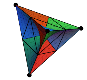
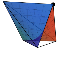
Figure 1: A $3$-dimensional slice of the $7$-dimensional model of $2{\times}2{\times}2$ tensors of nonnegative rank $\leq 2$. Each toric cell is bounded by $3$ quadrics and contains a vertex of the tetrahedron.

Example 2.16.

We consider $2\times 2\times 2$ tensors. Since secant lines of the Segre variety $\mathbb{P}^{1}{\times}\mathbb{P}^{1}{\times}\mathbb{P}^{1}$ fill all of $\mathbb{P}^{7}$, we have that $\mathcal{V}_{2}=\mathbb{P}^{7}$ and $\mathcal{M}_{2}=\Delta_{7}$. The mixture model ${\rm Mix}_{2}$ is an interesting, full-dimensional, closed, semi-algebraic subset of $\Delta_{7}$. By definition, ${\rm Mix}_{2}$ is the image of a 2-to-1 map $\phi:(\Delta_{1})^{7}\rightarrow\Delta_{7}$ analogous to (2.4). The branch locus is the $2{\times}2{\times}2$-hyperdeterminant, which is a hypersurface in $\mathbb{P}^{7}$ of degree $4$ and ML degree $13$.

The analysis in [1, §2] represents the model ${\rm Mix}_{2}$ as the union of four toric cells. One of these toric cells is the set of tensors satisfying

$$\begin{matrix}p_{111}p_{222}\geq p_{112}p_{221}&\quad p_{111}p_{222}\geq p_{121}p_{212}&\quad p_{111}p_{222}\geq p_{211}p_{122}\\ p_{112}p_{222}\geq p_{122}p_{212}&\quad p_{121}p_{222}\geq p_{122}p_{221}&\quad p_{211}p_{222}\geq p_{212}p_{221}\\ p_{111}p_{122}\geq p_{112}p_{121}&\quad p_{111}p_{212}\geq p_{112}p_{211}&\quad p_{111}p_{221}\geq p_{121}p_{211}\end{matrix}$$ (2.5)

A nonnegative $2{\times}2{\times}2$-tensor $P$ in $\Delta_{7}$ is supermodular if it satisfies these inequalities, possibly after label swapping $1\leftrightarrow 2$. We visualize ${\rm Mix}_{2}$ by restricting to the $3$-dimensional subspace $H$ given by $\,p_{111}=p_{222},\,p_{112}=p_{221},\,p_{121}=p_{212}\,$ and $\,p_{211}=p_{122}$. The intersection $H\cap\Delta_{7}$ is a tetrahedron, and we consider $H\cap{\rm Mix}_{2}$ inside that tetrahedron. The restricted model $H\cap{\rm Mix}_{2}$ is shown on the left in Figure 1. It consists of four toric cells as shown on the right side. The boundary is given by three quadratic surfaces, shown in red, green and blue, and which are obtained from either the first or the second row in (2.5) by restriction to $H$.

The boundary analysis suggested in Example 2.13 turns out to be quite simple in the present example. All boundary strata of the model ${\rm Mix}_{2}$ are varieties of ML degree $1$.

One such boundary stratum for ${\rm Mix}_{2}$ is the $5$-dimensional toric variety

$$X\,=\,V(p_{112}p_{222}-p_{122}p_{212},p_{111}p_{122}-p_{112}p_{121},p_{111}p_{222}-p_{121}p_{212})\,\,\,\subset\,\,\,\mathbb{P}^{7}.$$

As a preview for what is to come, we report its ML bidegree and its sectional ML degree:

$$\begin{matrix}B_{X}(p,u)&=&p^{7}\,+\,2p^{6}u\,+\,3p^{5}u^{2}\,+\,3p^{4}u^{3}\,+\,3p^{3}u^{4}\,+\,3p^{2}u^{5},\\ S_{X}(p,u)&=&p^{7}+14p^{6}u+30p^{5}u^{2}+30p^{4}u^{3}+15p^{3}u^{4}+3p^{2}u^{5}.\end{matrix}$$ (2.6)

In the next section, we shall study the class of toric varieties and the class of varieties having ML degree 1. Our variety $X$ lies in the intersection of these two important classes. $\diamondsuit$

3 Third Lecture

In our third lecture we start out with the likelihood geometry of embedded toric varieties. Fix a $(d{+}1)\times(n{+}1)$ integer matrix $A=(a_{0},a_{1},\ldots,a_{n})$ of rank $d{+}1$ that has $(1,1,\ldots,1)$ as its last row. This matrix defines an effective action of the torus $\,(\mathbb{C}^{*})^{d}$ on projective space $\mathbb{P}^{n}$:

$$(\mathbb{C}^{*})^{d}\times\mathbb{P}^{n}\longrightarrow\mathbb{P}^{n},\qquad t\times(p_{0}:p_{1}:\cdots:p_{n})\longmapsto(t^{\tilde{a}_{0}}\cdot p_{0}:t^{\tilde{a}_{1}}\cdot p_{1}:\cdots:t^{\tilde{a}_{n}}\cdot p_{n}).$$

Here $\tilde{a}_{i}$ is the column vector $a_{i}$ with the last entry $1$ removed. We also fix

$$c=(c_{0},c_{1},\ldots,c_{n})\in(\mathbb{C}^{*})^{n+1},$$

viewed as a point in $\mathbb{P}^{n}$. Let $X_{c}$ be the closure in $\mathbb{P}^{n}$ of the orbit $\,(\mathbb{C}^{*})^{d}\cdot c$. This is a projective toric variety of dimension $d$, defined by the pair $(A,c)$. The ideal that defines $X_{c}$ is the familiar toric ideal $I_{A}$ as in [15, §1.3], but with $p=(p_{0},\ldots,p_{n})$ replaced by

$$p/c\,\,=\,\,\biggl{(}\frac{p_{0}}{c_{0}},\frac{p_{1}}{c_{1}},\ldots,\frac{p_{n}}{c_{n}}\biggr{)}.$$ (3.1)

Example 3.1.

Fix $d=2$ and $n=3$. The matrix

$$A=\begin{pmatrix}0&3&0&1\\ 0&0&3&1\\ 1&1&1&1\end{pmatrix}$$

specifies the following family of toric surfaces of degree three in $\mathbb{P}^{3}$:

$$X_{c}\,\,=\,\,\overline{\{(c_{0}:c_{1}x_{1}^{3}:c_{2}x_{2}^{3}:c_{3}x_{1}x_{2})\,:(x_{1},x_{2})\in(\mathbb{C}^{*})^{2}\}}\\ \,\,=\,\,V(c_{3}^{3}\cdot p_{0}p_{1}p_{2}\,-\,c_{0}c_{1}c_{2}\cdot p_{3}^{3}).$$

Of course, the prime ideal of any particular surface $X_{c}$ is the principal ideal generated by

$$\frac{p_{0}}{c_{0}}\frac{p_{1}}{c_{1}}\frac{p_{2}}{c_{2}}\,-\,\biggl{(}\frac{p_{3}}{c_{3}}\biggr{)}^{3}.$$

How does the ML degree of $X_{c}$ depend on the parameter $c=(c_{0},c_{1},c_{2},c_{3})\in(\mathbb{C}^{*})^{4}$? $\diamondsuit$

We shall express the ML degree of the toric variety $X_{c}$ in terms of the complement of a hypersurface in the torus $(\mathbb{C}^{*})^{d}$. The pair $(A,c)$ define the sparse Laurent polynomial

$$f(x)\,\,=\,\,c_{0}\cdot x^{\tilde{a}_{0}}+c_{1}\cdot x^{\tilde{a}_{1}}+\cdots+c_{n}\cdot x^{\tilde{a}_{n}}.$$

Theorem 3.2.

The ML degree of the $d$-dimensional toric variety $\,X_{c}\subset\mathbb{P}^{n}\,$ is equal to $(-1)^{d}$ times the Euler characteristic of the very affine variety

$$X_{c}\backslash\mathcal{H}\,\,\,\simeq\,\,\,\bigl{\{}x\in(\mathbb{C}^{*})^{d}\,:\,f(x)\not=0\bigr{\}}.$$ (3.2)

For generic $c$, the ML degree agrees with the degree of $X_{c}$, which is the normalized volume of the $d$-dimensional lattice polytope ${\rm conv}(A)$ obtained as the convex hull of the columns of $A$.

Proof.

We first argue that the identification (3.2) holds. The map

$$x\,\,\longmapsto\,\,{p}\,=\,(c_{0}\cdot{x}^{\tilde{a}_{0}}:c_{1}\cdot x^{\tilde{a}_{1}}:\cdots:c_{n}\cdot{x}^{\tilde{a}_{n}})$$

defines an injective group homomorphism from $(\mathbb{C}^{*})^{d}$ into the dense torus of $\mathbb{P}^{n}$. Its image is equal to the dense torus of $X_{c}$, so we have an isomorphism between $(\mathbb{C}^{*})^{d}$ and the dense torus of $X_{c}$. Under this isomorphism, the affine open set $\{f\not=0\}$ in $(\mathbb{C}^{*})^{d}$ is identified with the affine open set $\{p_{0}+\cdots+p_{n}\not=0\}$ in the dense torus of $X_{c}$. The latter is precisely $X_{c}\backslash\mathcal{H}$. Since $(\mathbb{C}^{*})^{d}$ is smooth, we see that $X_{c}\backslash\mathcal{H}$ is smooth, so our first assertion follows from Theorem 1.7. The second assertion is a consequence of the description of the likelihood correspondence $\mathcal{L}_{X_{c}}$ via linear sections of $X_{{c}}$ that is given in Proposition 3.5 below. ∎

Example 3.3.

We return to the cubic surface $X_{c}$ in Example 3.1. For a general parameter vector ${c}$, the ML degree of $X_{{c}}$ is $3$. For instance, the surface $V(p_{0}p_{1}p_{2}-p_{3}^{3})\subset\mathbb{P}^{3}$ has ML degree $3$. However, the ML degree of $X_{{c}}$ drops to $2$ whenever the plane curve defined by

$$f(x_{1},x_{2})=c_{0}+c_{1}x_{1}^{3}+c_{2}x_{2}^{3}+c_{3}x_{1}x_{2}\,$$

has a singularity in $(\mathbb{C}^{*})^{2}$. For instance, this happens for $c=(1:1:1:-3)$. The corresponding surface $V(27p_{0}p_{1}p_{2}+p_{3}^{3})\subset\mathbb{P}^{3}$ has ML degree $2$. $\diamondsuit$

The isomorphism (3.2) has a nice interpretation in terms of Convex Optimization. Namely, it implies that maximum likelihood estimation for toric varieties is equivalent to global minimization of posynomials, and hence to the most fundamental case of Geometric Programming. We refer to [9, §4.5] for an introduction to posynomials and geometric programming.

We write $|\,\cdot\,|$ for the 1-norm on $\mathbb{R}^{n+1}$, we set ${b}=A{u}$, and we assume that ${c}=(c_{0},c_{1},\ldots,c_{n})$ is in $\mathbb{R}_{>0}^{n+1}$. Maximum likelihood estimation for toric models is the problem

$${\rm Maximize}\,\,\,\,\frac{p^{u}}{|p|^{|{u}|}}\,\,\,\,\hbox{subject to}\,\,\,p\,\in\,X_{c}\cap\Delta_{n}.$$ (3.3)

Setting $p_{i}=c_{i}\cdot{x}^{{\tilde{a}_{i}}}$ as above, this problem becomes equivalent to the geometric program

$${\rm Minimize}\,\,\,\,\frac{f({x})^{|{u}|}}{{x}^{b}}\,\,\,\,\hbox{subject to}\,\,\,{x}\in\mathbb{R}_{>0}^{d}.$$ (3.4)

By construction, $f({x})^{|{u}|}/{x}^{b}$ is a posynomial whose Newton polytope contains the origin. Such a posynomial attains a unique global minimum on the open orthant $\mathbb{R}^{d}_{>0}$. This can be seen by convexifying as in [9, §4.5.3]. This global minimum of (3.4) corresponds to the solution of (3.3), which exists and is unique by Birch’s Theorem [37, Theorem 1.10].

Example 3.4.

Consider the geometric program for the surfaces in Example 3.1, with

$$A\,=\,\begin{pmatrix}\,0&3&0&1\,\\ \,0&0&3&1\,\\ \,1&1&1&1\,\end{pmatrix}\quad\hbox{and}\quad{u}\,=\,(0,0,0,1).$$

The problem (3.4) is to find the global minimum, over all positive $x=(x_{1},x_{2})$, of the function

$$\frac{f(x_{1},x_{2})}{x_{1}x_{2}}\,\,=\,\,c_{0}x_{1}^{-1}x_{2}^{-1}+c_{1}x_{1}^{2}x_{2}^{-1}+c_{2}x_{1}^{-1}x_{2}^{2}+c_{3}.$$

This is equivalent to maximizing $p_{3}/p_{+}$ subject to $\,{p}\in V(c_{3}^{3}\cdot p_{0}p_{1}p_{2}\,-\,c_{0}c_{1}c_{2}\cdot p_{3}^{3})\cap\Delta_{3}$. $\diamondsuit$

We now describe the toric likelihood correspondence $\mathcal{L}_{X_{c}}$ in $\mathbb{P}^{n}\times\mathbb{P}^{n}$ associated with the pair $(A,{c})$. This is the likelihood correspondence of the toric variety $X_{c}\subset\mathbb{P}^{n}$ defined above.

Proposition 3.5.

On the open subset $\,(X_{c}\backslash\mathcal{H})\times\mathbb{P}^{n}$, the toric likelihood correspondence $\mathcal{L}_{X_{c}}$ is defined by the $2\times 2$-minors of the $2\times(d{+}1)$-matrix

$$\begin{pmatrix}{p}/{c}\cdot A^{T}\\ {u}/{c}\cdot A^{T}\end{pmatrix}.$$ (3.5)

Here the notation ${p}/{c}$ is as in (3.1). In particular, for any fixed data vector ${u}$, the critical points of $\ell_{u}$ are characterized by a linear system of equations in ${p}$ restricted to $X_{c}$.

Proof.

This is an immediate consequence of Birch’s Theorem [37, Theorem 1.10]. ∎

Example 3.6.

The Hardy-Weinberg curve of Example 1.3 is the subvariety $\,X_{c}=V(p_{1}^{2}-4p_{0}p_{2})\,$ in the projective plane $\mathbb{P}^{2}$. As a toric variety, this plane curve is given by

$$A=\begin{pmatrix}0&1&2\\ 2&1&0\end{pmatrix}\quad\hbox{and}\quad\,{c}=(1,2,1).$$

The likelihood correspondence of $X_{c}$ is the surface in $\mathbb{P}^{2}\times\mathbb{P}^{2}$ given by

$${\rm det}\begin{pmatrix}2p_{0}&p_{1}\\ p_{1}&2p_{2}\end{pmatrix}\,\,=\,\,{\rm det}\begin{pmatrix}p_{1}+2p_{2}&2p_{0}+p_{1}\\ u_{1}+2u_{2}&2u_{0}+u_{1}\end{pmatrix}\,\,=\,\,0.$$ (3.6)

Note that the second determinant equals the determinant of the $2\times 2$-matrix (3.5) times $4$. Saturating (3.6) with respect to $p_{0}+p_{1}+p_{2}$ reveals two further equations of degree $(1,1)$:

$$2(u_{1}+2u_{2})p_{0}=(2u_{0}+u_{1})p_{1}\quad\hbox{and}\quad(u_{1}+2u_{2})p_{1}=2(2u_{0}+u_{1})p_{2}.$$

For fixed ${u}$, these equations have a unique solution in $\mathbb{P}^{2}$, given by the formula in (1.3). $\diamondsuit$

Toric varieties are rational varieties that are parametrized by monomials. We now examine those varieties that are parametrized by generic polynomials. Understanding these is useful for statistics since many widely used models for discrete data are given in the form

$$f:\Theta\rightarrow\Delta_{n},$$

where $\Theta$ is a $d$-dimensional polytope and $f$ is a polynomial map. The coordinates $f_{0},f_{1},\ldots,f_{n}$ are polynomial functions in the parameters $\theta=(\theta_{1},\ldots,\theta_{d})$ satisfying $\,f_{0}+f_{1}+\cdots+f_{n}=1$. Such models include the mixture models in Proposition 2.11, phylogenetic models, Bayesian networks, hidden Markov models, and many others arising in computational biology [37].

The model specified by the polynomials $f_{0},\ldots,f_{n}$ is the semialgebraic set $f(\Theta)\subset\Delta_{n}$. We study its Zariski closure $\,X=\overline{f(\Theta)}\,$ in $\mathbb{P}^{n}$. Finding its equations is hard and interesting.

Theorem 3.7.

Let $f_{0},f_{1},\ldots,f_{n}$ be polynomials of degrees $b_{0},b_{1},\ldots,b_{n}$ satisfying $\sum f_{i}=1$. The ML degree of the variety $X$ is at most the coefficient of $z^{d}$ in the generating function

$$\frac{(1-z)^{d}}{(1-zb_{0})(1-zb_{1})\cdots(1-zb_{n})}.$$

Equality holds when the coefficients of $f_{0},f_{1},\ldots,f_{n}$ are generic relative to $\sum f_{i}=1$.

Proof.

This is the content of [10, Theorem 1]. ∎

Example 3.8.

We examine the case of quartic surfaces in $\mathbb{P}^{3}$. Let $d=2,n=3$, pick random affine quadrics $f_{1},f_{2},f_{3}$ in two unknowns and set $f_{0}=1-f_{1}-f_{2}-f_{3}$. This defines a map

$$f\,:\,\mathbb{C}^{2}\rightarrow\mathbb{C}^{3}\subset\mathbb{P}^{3}.$$

The ML degree of the image surface $X=\overline{f(\mathbb{C}^{2})}$ in $\mathbb{P}^{3}$ is equal to $25$ since

$$\frac{(1-z)^{2}}{(1-2z)^{4}}\,=\,1+6z+{\bf 25}z^{2}+88z^{3}+\cdots$$

The rational surface $X$ is a Steiner surface (or Roman surface). Its singular locus consists of three lines that meet in a point $P$. To understand the graph of $f$, we observe that the linear span of $\{f_{0},f_{1},f_{2},f_{3}\}$ in $\mathbb{C}[x,y]$ has a basis $\{1,L^{2},M^{2},N^{2}\}$ where $L,M,N$ represent lines in $\mathbb{C}^{2}$. Let $l$ denote the line through $M\cap N$ parallel to $L$, $m$ the line through $L\cap N$ parallel to $M$, and $n$ the line through $L\cap M$ parallel to $N$. The map $\mathbb{C}^{2}\rightarrow X$ is a bijection outside these three lines, and it maps each line 2-to-1 onto one of the lines in $X_{\rm sing}$. The fiber over the special point $P$ on $X$ consists of three points, namely, $l\cap m$, $l\cap n$ and $m\cap n$. If the quadric $f_{0}$ were also picked at random, rather than as $1-f_{1}-f_{2}-f_{3}$, then we would still get a Steiner surface $X\subset\mathbb{P}^{3}$. However, now the ML degree of $X$ increases to $33$.

On the other hand, if we take $X$ to be a general quartic surface in $\mathbb{P}^{3}$, so $X$ is a smooth K3 surface of Picard rank $1$, then $X$ has ML degree $84$. This is the formula in Example 1.11 evaluated at $n=3$ and $d=4$. Here $X\backslash\mathcal{H}$ is the generic quartic surface in $\mathbb{P}^{3}$ with five plane sections removed. The number $84$ is the Euler characteristic of that open K3 surface.

In the first case, $X\backslash\mathcal{H}$ is singular, so we cannot apply Theorem 1.7 directly to our Steiner surface $X$ in $\mathbb{P}^{3}$. However, we can work in the parameter space and consider the smooth very affine surface $\mathbb{C}^{2}\backslash V(f_{0}f_{1}f_{2}f_{3})$. The number $25$ is the Euler characteristic of that surface.

It is instructive to verify Conjecture 1.8 for our three quartic surfaces in $\mathbb{P}^{3}$. We found

$$\begin{matrix}\chi(X\backslash\mathcal{H})&=&38&&>&&25&=&{\rm MLdegree}\,(X),\\ \chi(X\backslash\mathcal{H})&=&49&&>&&33&=&{\rm MLdegree}\,(X),\\ \chi(X\backslash\mathcal{H})&=&84&&=&&84&=&{\rm MLdegree}\,(X).\end{matrix}$$

The Euler characteristics of the three surfaces were computed using Aluffi’s method [2]. $\diamondsuit$

We now turn to the following question: which projective varieties $X$ have ML degree one? This question is important for likelihood inference because a model having ML degree one means that the MLE $\hat{p}$ is a rational function in the data $u$. It is known that Bayesian networks and decomposable graphical models enjoy this property, and it is natural to wonder which other statistical models are in this class. The answer to this question was given by the first author in [27]. We shall here present the result of [27] from a slightly different angle.

Our point of departure is the notion of the $A$-discriminant, as introduced and studied by Gel’fand, Kapranov and Zelevinsky in [19]. We fix an $r\times m$ integer matrix $A=(a_{1},a_{2},\ldots,a_{m})$ of rank $r$ which has $(1,1,\ldots,1)$ in its row space. The Zariski closure of

$$\bigl{\{}({t}^{a_{1}}:{t}^{a_{2}}:\cdots:{t}^{a_{m}})\,\in\mathbb{P}^{m-1}\,\,:\,\,{t}\in(\mathbb{C}^{*})^{r}\bigr{\}}$$

is an $(r-1)$-dimensional toric variety $Y_{A}$ in $\mathbb{P}^{m-1}$. We here intentionally changed the notation relative to that used for toric varieties at the beginning of this section. The reason is that $d$ and $n$ are always reserved for the dimension and embedding dimension of a statistical model.

The dual variety $\,Y_{A}^{*}\,$ is an irreducible variety in the dual projective space $(\mathbb{P}^{m-1})^{\vee}$ whose coordinates are ${x}=(x_{1}:x_{2}:\cdots:x_{m})$. We identify points ${x}$ in $(\mathbb{P}^{m-1})^{\vee}$ with hypersurfaces

$$\bigl{\{}\,{t}\in(\mathbb{C}^{*})^{r}\,\,:\,\,x_{1}\cdot{t}^{a_{1}}+x_{2}\cdot{t}^{a_{2}}+\cdots+x_{m}\cdot{t}^{a_{m}}\,\,=\,\,0\,\bigr{\}}.$$ (3.7)

The dual variety $Y_{A}^{*}$ is the Zariski closure in $(\mathbb{P}^{m-1})^{\vee}$ of the locus of all hypersurfaces (3.7) that are singular. Typically, $Y_{A}^{*}$ is a hypersurface. In that case, $Y_{A}^{*}$ is defined by a unique (up to sign) irreducible polynomial ${\Delta_{A}}\in\mathbb{Z}[x_{1},x_{2},\ldots,x_{m}]$. The homogeneous polynomial $\,{\Delta_{A}}\,$ is called the $A$-discriminant. Many classical discriminants and resultants are instances of $\Delta_{A}$. So are determinants and hyperdeterminants. This is the punch line of the book [19].

Example 3.9.

Let $m=4,r=2$, and $A=\begin{pmatrix}3&2&1&0\\ 0&1&2&3\end{pmatrix}$. The associated toric variety is the twisted cubic curve

$$Y_{A}=\overline{\bigl{\{}(1:t:t^{2}:t^{3})\,|\,t\in\mathbb{C}\bigr{\}}}\,\subset\mathbb{P}^{3}.$$

The variety $Y_{A}^{*}$ that is dual to the curve $Y_{A}$ is a surface in $(\mathbb{P}^{3})^{\vee}$. The surface $Y_{A}^{*}$ parametrizes all planes that are tangent to the curve $Y_{A}$. These represent univariate cubics

$$x_{1}+x_{2}t+x_{3}t^{2}+x_{4}t^{3}$$

that have a double root. Here the $A$-discriminant is the classical discriminant

$$\Delta_{A}\,=\,27x_{1}^{2}x_{4}^{2}-18x_{1}x_{2}x_{3}x_{4}+4x_{1}x_{3}^{3}+4x_{2}^{3}x_{4}-x_{2}^{2}x_{3}^{2}.$$

The surface $Y_{A}^{*}$ in $\mathbb{P}^{3}$ defined by this equation is the discriminant of the univariate cubic. $\diamondsuit$

Theorem 3.10.

Let $X\subseteq\mathbb{P}^{n}$ be a projective variety of ML degree $1$. Each coordinate $\hat{p}_{i}$ of the rational function $\,u\mapsto\hat{p}\,$ is an alternating product of linear forms in $u_{0},u_{1},\ldots,u_{n}$.

The paper [27] gives an explicit construction of the map $u\mapsto\hat{p}$ as a Horn uniformization. A precursor was [28]. We explain this construction. The point of departure is a matrix $A$ as above. We now take $\Delta_{A}$ to be any non-zero homogenous polynomial that vanishes on the dual variety $Y_{A}^{*}$ of the toric variety $Y_{A}$. If $Y_{A}^{*}$ is a hypersurface then $\Delta_{A}$ is the $A$-discriminant.

First, we write $\Delta_{A}$ as a Laurent polynomial by dividing it by one of its monomials:

$$\frac{1}{\rm monomial}\cdot\Delta_{A}\,\,\,=\,\,\,1\,-\,c_{0}\cdot{x}^{b_{0}}\,-\,c_{1}\cdot{x}^{b_{1}}\,-\,\cdots\,-\,c_{n}\cdot{x}^{b_{n}}.$$ (3.8)

This expression defines an $m\times(n+1)$ integer matrix $B=(b_{0},\ldots,b_{n})$ satisfying $AB=0$. Second, we define $X$ to be the rational subvariety of $\mathbb{P}^{n}$ that is given parametrically by

$$\frac{p_{i}}{p_{0}+p_{1}+\cdots+p_{n}}\,\,\,=\,\,\,c_{i}\cdot{x}^{b_{i}}\qquad\hbox{for}\,\,\,i=0,1,\ldots,n.$$ (3.9)

The defining ideal of $X$ is obtained by eliminating $x_{1},\ldots,x_{m}$ from the equations above. Then $X$ has ML degree $1$, and, by [27], every variety of ML degree $1$ arises in this manner.

Example 3.11.

The following curve in $\mathbb{P}^{3}$ happens to be a variety of ML degree $1$:

$$X\,\,=\,\,V\bigl{(}\,9p_{1}p_{2}-8p_{0}p_{3}\,,\,p_{0}^{2}-12(p_{0}{+}p_{1}{+}p_{2}{+}p_{3})p_{3}\,\bigr{)}.$$

This curve comes from the discriminant of the univariate cubic in Example 3.9:

$$\frac{1}{{\rm monomial}}\cdot\Delta_{A}\,\,=\,\,1-\bigl{(}\frac{2}{3}\frac{x_{2}x_{3}}{x_{1}x_{4}}\bigr{)}-\bigl{(}-\frac{4}{27}\frac{x_{2}^{3}}{x_{1}^{2}x_{4}}\bigr{)}-\bigl{(}-\frac{4}{27}\frac{x_{3}^{3}}{x_{1}x_{4}^{2}}\bigr{)}-\bigl{(}\frac{1}{27}\frac{x_{2}^{2}x_{3}^{2}}{x_{1}^{2}x_{4}^{2}}\bigr{)}.$$

We derived the curve $X$ from the four parenthesized monomials via the formula (3.9). The maximum likelihood estimate for this model is given by the products of linear forms

$$\hat{p}_{0}=\frac{2}{3}\frac{x_{2}x_{3}}{x_{1}x_{4}}\qquad\hat{p}_{1}=-\frac{4}{27}\frac{x_{2}^{3}}{x_{1}^{2}x_{4}}\qquad\hat{p}_{2}=-\frac{4}{27}\frac{x_{3}^{3}}{x_{1}x_{4}^{2}}\qquad\hat{p}_{3}=\frac{1}{27}\frac{x_{2}^{2}x_{3}^{2}}{x_{1}^{2}x_{4}^{2}}$$

where

$$\begin{matrix}x_{1}&=&-u_{0}-u_{1}-2u_{2}-2u_{3}&&x_{2}&=&u_{0}+3u_{2}+2u_{3}\\ x_{3}&=&u_{0}+3u_{1}+2u_{3}&&x_{4}&=&-u_{0}-2u_{1}-u_{2}-2u_{3}\end{matrix}$$

These expressions are the alternating products of linear forms promised in Theorem 3.10. $\diamondsuit$

We now give the formula for $\hat{p}_{i}$ in general. This is the Horn uniformization of [19, §9.3].

Corollary 3.12.

Let $X\subset\mathbb{P}^{n}$ be the variety of ML degree $1$ with parametrization (3.9) derived from a scaled $A$-discriminant (3.8). The coordinates of the MLE function $u\mapsto\hat{p}$ are

$$\hat{p}_{k}\quad=\quad c_{k}\cdot\prod_{j=1}^{m}(\sum_{i=0}^{n}b_{ij}u_{i})^{b_{kj}}.$$

It is not obvious (but true) that $\,\hat{p}_{0}+\hat{p}_{1}+\cdots+\hat{p}_{n}=1\,$ holds in the formula above. In light of its monomial parametrization, our variety $X$ is toric in $\mathbb{P}^{n}\backslash\mathcal{H}$. In general, it is not toric in $\mathbb{P}^{n}$, due to appearances of the factor $(p_{0}+p_{1}+\cdots+p_{n})$ in equations for $X$. Interestingly, there are numerous instances when this factor does not appear and $X$ is toric also in $\mathbb{P}^{n}$.

One toric instance is the independence model $\,X=V(p_{00}p_{11}-p_{01}p_{10})$, whose MLE was derived in Example 1.14. What is the matrix $A$ in this case? We shall answer this question for a slightly larger example, which serves as an illustration for decomposable graphical models.

Example 3.13.

Consider the conditional independence model for three binary variables given by the graph   $\bullet$—–$\bullet$—–$\bullet$. We claim that this graphical model is derived from

$$A\,\,\,=\,\,\bordermatrix{&a_{00}&a_{10}&a_{01}&a_{11}&b_{00}&b_{01}&b_{10}&b_{11}&c_{0}&c_{1}&d\cr&1&1&1&1&1&1&1&1&1&1&1\cr x\!&1&1&0&0&0&0&0&0&1&0&0\cr y\!&0&0&1&1&0&0&0&0&0&1&0\cr z\!&0&0&0&0&1&1&0&0&1&0&0\cr w\!&0&0&0&0&0&0&1&1&0&1&0\cr}.$$

The discriminant of the corresponding family of hypersurfaces

$$\bigl{\{}(x,y,z,w)\in(\mathbb{C}^{*})^{4}\,|\,(a_{00}+a_{10})x+(a_{01}+a_{11})y+(b_{00}+b_{01})z+(b_{10}+b_{11})w+c_{0}xz+c_{1}yw+d=0\bigr{\}}$$

equals

$$\begin{matrix}\Delta_{A}&=&c_{0}c_{1}d-a_{01}b_{10}c_{0}-a_{11}b_{10}c_{0}-a_{01}b_{11}c_{0}-a_{11}b_{11}c_{0}\\ &&-a_{00}b_{00}c_{1}-a_{10}b_{00}c_{1}-a_{00}b_{01}c_{1}-a_{10}b_{01}c_{1}.\end{matrix}$$

We divide this $A$-discriminant by its first term $\,c_{0}c_{1}d\,$ to rewrite it in the form (3.8) with $n=7$. The parametrization of $X\subset\mathbb{P}^{7}$ given by (3.9) can be expressed as

$$\quad p_{ijk}\,=\,\frac{a_{ij}\cdot b_{jk}}{c_{j}\cdot d}\quad\qquad\hbox{for}\,\,i,j,k\in\{0,1\}.$$ (3.10)

This is indeed the desired graphical model  $\bullet$—–$\bullet$—–$\bullet$  with implicit representation

$$X\,\,=\,\,V\bigl{(}p_{000}p_{101}-p_{001}p_{100}\,,\,p_{010}p_{111}-p_{011}p_{110}\bigr{)}\,\,\,\subset\,\,\,\mathbb{P}^{7}.$$

The linear forms used in the Horn uniformization of Corollary 3.12 are

$$a_{ij}=u_{ij+}\qquad b_{jk}=u_{+jk}\qquad c_{j}=u_{+j+}\qquad d=u_{+++}$$

Substituting these expressions into (3.10), we obtain

$$\qquad\hat{p}_{ijk}\,\,=\,\,\frac{u_{ij+}\cdot u_{+jk}}{u_{+j+}\cdot u_{+++}}\qquad\hbox{for}\,\,i,j,k\in\{0,1\}.$$

This is the formula in Lauritzen’s book [32] for MLE of decomposable graphical models. $\diamondsuit$

We now return to the likelihood geometry of an arbitrary $d$-dimensional projective variety $X$ in $\mathbb{P}^{n}$, as always defined over $\mathbb{R}$ and not contained in $\mathcal{H}$. We define the ML bidegree of $X$ to be the bidegree of its likelihood correspondence $\mathcal{L}_{X}\subset\mathbb{P}^{n}\times\mathbb{P}^{n}$. This is a binary form

$$B_{X}(p,u)\quad=\quad(b_{0}\cdot p^{d}+b_{1}\cdot p^{d-1}u+\cdots+b_{d}\cdot u^{d})\cdot p^{n-d},$$

where $b_{0},b_{1},\ldots,b_{d}$ are certain positive integers. By definition, $B_{X}(p,u)$ is the multidegree [33, §8.5] of the prime ideal of $\mathcal{L}_{X}$, with respect to the natural $\mathbb{Z}^{2}$-grading on the polynomial ring $\mathbb{R}[p,u]=\mathbb{R}[p_{0},\ldots,p_{n},u_{0},\ldots,u_{n}]$. Equivalently, the ML bidegree $B_{X}(p,u)$ is the class defined by $\mathcal{L}_{X}$ in the cohomology ring

$$H^{*}(\mathbb{P}^{n}\times\mathbb{P}^{n};\mathbb{Z})=\mathbb{Z}[p,u]/\langle p^{n+1},u^{n+1}\rangle.$$

We already saw some examples, for the Grassmannian $G(2,4)$ in (1.12), for arbitrary linear spaces in (1.14), and for a toric model of ML degree $1$ in (2.6). We note that the bidegree $B_{X}(p,u)$ can be computed conveniently using the command multidegree in Macaulay2.

To understand the geometric meaning of the ML bidegree, we introduce a second polynomial. Let $L_{n-i}$ be a sufficiently general linear subspace of $\mathbb{P}^{n}$ of codimension $i$, and define

$$s_{i}\,=\,\text{MLdegree}\,(X\cap L_{n-i}).$$

We define the sectional ML degree of $X$ to be the polynomial

$$S_{X}(p,u)\quad=\quad(s_{0}\cdot p^{d}+s_{1}\cdot p^{d-1}u+\cdots+s_{d}\cdot u^{d})\cdot p^{n-d},$$

Example 3.14.

The sectional ML degree of the Grassmannian $G(2,4)$ in (1.10) equals

$$S_{X}(p,u)\,\,=\,\,4p^{5}+20p^{4}u+24p^{3}u^{2}+12p^{2}u^{3}+2pu^{4}.$$

Thus, if $H_{1},H_{2},H_{3}$ denote generic hyperplanes in $\mathbb{P}^{5}$, then the threefold $G(2,4)\cap H_{1}$ has ML degree $20$, the surface $G(2,4)\cap H_{1}\cap H_{2}$ has ML degree $24$, and the curve $G(2,4)\cap H_{1}\cap H_{2}\cap H_{3}$ has ML degree $12$. Lastly, the coefficient $2$ of $pu^{4}$ is simply the degree of $G(2,4)$ in $\mathbb{P}^{5}$. $\diamondsuit$

Conjecture 3.15.

The ML bidegree and the sectional ML degree of any projective variety $X\subset\mathbb{P}^{n}$, not lying in $\mathcal{H}$, are related by the following involution on binary forms of degree $n$:

$$B_{X}(p,u) = \frac{u\cdot S_{X}(p,u-p)-p\cdot S_{X}(p,0)}{u-p},$$

$$S_{X}(p,u) = \frac{u\cdot B_{X}(p,u+p)+p\cdot B_{X}(p,0)}{u+p}.$$

This conjecture is a theorem when $X\backslash\mathcal{H}$ is smooth and its boundary is schön. See Theorem 4.6 below. In that case, the ML bidegree is identified, by [25, Theorem 2], with the Chern-Schwartz-MacPherson (CSM) class of the constructible function on $\mathbb{P}^{n}$ that is $1$ on $X\backslash\mathcal{H}$ and $0$ elsewhere. Aluffi proved in [4, Theorem 1.1] that the CSM class of an locally closed subset of $\mathbb{P}^{n}$ satisfies such a log-adjunction formula. Our formula in Conjecture 3.15 is precisely the homogenization of Aluffi’s involution. The combination of [4, Theorem 1.1] and [25, Theorem 2] proves Conjecture 3.15 in cases such as generic complete intersections (Theorem 1.10) and arbitrary linear spaces (Theorem 1.20). In the latter case, it can also be verified using matroid theory. Conjecture 3.15 says that this holds for any $X$, indicating a deeper connection between likelihood correspondences and CSM classes.

We note that $B_{X}(p,u)$ and $S_{X}(p,u)$ always share the same leading term and the same trailing term, and this is compatible with our formulas. Both polynomials start and end like

$${\rm MLdegree}\,(X)\cdot p^{n}\,+\,\cdots\,+{\rm degree}\,(X)\cdot p^{{\rm codim}(X)}u^{{\rm dim}(X)}.$$

We now illustrate Conjecture 3.15 by verifying it computationally for a few more examples.

Example 3.16.

Let us examine some cubic fourfolds in $\mathbb{P}^{5}$. If $X$ is a generic hypersurface of degree $4$ in $\mathbb{P}^{5}$ then its sectional ML degree and ML bidegree satisfy the conjectured formula:

$$\begin{matrix}S_{X}(p,u)&=&1364p^{5}\,+\,448p^{4}u\,+\,136p^{3}u^{2}\,+\,32p^{2}u^{3}\,+\,3pu^{4},\\ B_{X}(p,u)&=&1364p^{5}\,+\,341p^{4}u\,+\,81p^{3}u^{2}\,+\,23p^{2}u^{3}\,+\,3pu^{4}.\end{matrix}$$

Of course, in algebraic statistics, we are more interested in special hypersurfaces that are statistically meaningful. One such instance was seen in Example 2.7. The mixture model for two identically distributed ternary random variables is the fourfold $X\subset\mathbb{P}^{5}$ defined by

$${\rm det}\begin{pmatrix}2p_{11}&p_{12}&p_{13}\\ p_{12}&2p_{22}&p_{23}\\ p_{13}&p_{23}&2p_{33}\end{pmatrix}\quad=\quad 0.$$ (3.11)

The sectional ML degree and the ML bidegree of this determinantal fourfold are

$$\begin{matrix}S_{X}(p,u)&=&6p^{5}\,+\,42p^{4}u\,+\,48p^{3}u^{2}\,+\,21p^{2}u^{3}\,+\,3pu^{4}\\ B_{X}(p,u)&=&6p^{5}\,+\,12p^{4}u\,+\,15p^{3}u^{2}\,+\,12p^{2}u^{3}\,+\,3pu^{4}.\end{matrix}$$

For the toric fourfold $X=V(p_{11}p_{22}p_{33}\,{-}\,p_{12}p_{13}p_{23})$, ML bidegree and sectional ML degree are

$$\begin{matrix}B_{X}(p,u)&=&{\bf 3}p^{5}\,+\,3p^{4}u\,+\,3p^{3}u^{2}\,+\,3p^{2}u^{3}\,+\,3pu^{4},\\ S_{X}(p,u)&=&{\bf 3}p^{5}+12p^{4}u+18p^{3}u^{2}+12p^{2}u^{3}+3pu^{4}.\end{matrix}$$

Now, taking $X=V(p_{11}p_{22}p_{33}{+}p_{12}p_{13}p_{23})$ instead, the leading coefficient $3$ changes to $2$. $\diamondsuit$

Remark 3.17.

Conjecture 3.15 is true when $X_{c}$ is a toric variety with ${c}$ generic, as in Theorem 3.2. Here we can use Proposition 3.5 to infer that all coefficients of $B_{X}$ are equal to the normalized volume of the lattice polytope ${\rm conv}(A)$. In symbols, for generic ${c}$, we have

$$B_{X_{c}}(p,u)\quad=\quad{\rm degree}\,(X_{c})\cdot\sum_{i=0}^{d}p^{n-i}u^{i}.$$

It is now an exercise to transform this into a formula for the sectional ML degree $S_{X_{c}}(p,u)$.

In general, it is hard to compute generators for the ideal of the likelihood correspondence.

Example 3.18.

The following submodel of (3.11) was featured prominently in [23, §1]:

$${\rm det}\begin{pmatrix}12p_{0}&3p_{1}&2p_{2}\\ 3p_{1}&2p_{2}&3p_{3}\\ 2p_{2}&3p_{3}&12p_{4}\end{pmatrix}\quad=\quad 0.$$ (3.12)

This cubic threefold $X$ is the secant variety of a rational normal curve in $\mathbb{P}^{4}$, and it represents the mixture model for a binomial random variable (tossing a biased coin four times). It takes several hours in Macaulay2 to compute the prime ideal of the likelihood correspondence $\mathcal{L}_{X}\subset\mathbb{P}^{4}\times\mathbb{P}^{4}$. That ideal has $20$ minimal generators one in degree $(1,1)$, one in degree $(3,0)$, five in degree $(3,1)$, ten in degree $(4,1)$ and three in degree $(3,2)$. After passing to a Gröbner basis, we use the formula in [33, Definition 8.45] to compute the bidegree of $\mathcal{L}_{X}$:

$$B_{X}(p,u)\quad=\quad 12p^{4}+15p^{3}u+12p^{2}u^{2}+3pu^{3}.$$

We now intersect $X$ with random hyperplanes in $\mathbb{P}^{4}$, and we compute the ML degrees of the intersections. Repeating this experiment many times reveals the sectional ML degree of $X$:

$$S_{X}(p,u)\quad=\quad 12p^{4}+30p^{3}u+18p^{2}u^{2}+3pu^{3}.$$

The two polynomials satisfy our transformation rule, thus confirming Conjecture 3.15. We note that Conjecture 1.8 also holds for this example: using Aluffi’s method [2], we find $\chi(X\backslash\mathcal{H})=-13$. $\diamondsuit$

Our last topic is the operation of restriction and deletion. This is a standard tool for complements of hyperplane arrangements, as in Theorem 1.20. It was developed in [25] for arbitrary very affine varieties, such as $X\backslash\mathcal{H}$. We motivate this by explaining the distinction between structural zeros and sampling zeros for contingency tables in statistics [8, §5.1.1].

Returning to the “hair loss due to TV soccer” example from the beginning of Section 2, let us consider the following questions. What is the difference between the data set

$$U\quad\,=\,\,\,\,\bordermatrix{&\hbox{lots of hair}&\hbox{medium hair}&\hbox{little hair}\cr\hbox{$\leq 2$ hrs}&15&0&9\cr\hbox{$2$--$6$ hrs}&20&24&12\cr\hbox{$\geq 6$ hrs}&10&12&6}$$

and the data set

$$\tilde{U}\quad\,=\,\,\,\,\bordermatrix{&\hbox{lots of hair}&\hbox{medium hair}&\hbox{little hair}\cr\hbox{$\leq 2$ hrs}&10&0&5\cr\hbox{$2$--$6$ hrs}&9&3&6\cr\hbox{$\geq 6$ hrs}&7&9&8}\ ?$$

How should we think about the zero entries in row 1 and column 2 of these two contingency tables? Would the rank 1 model $\mathcal{M}_{1}$ or the rank 2 model $\mathcal{M}_{2}$ be more appropriate?

The first matrix $U$ has rank $2$ and it can be completed to a rank $1$ matrix by replacing the zero entry with $18$. Thus, the model $\mathcal{M}_{1}$ fits perfectly except for the structural zero in row 1 and column 2. It seems that this zero is inherent in the structure of the problem: planet Earth simply has no people with medium hair length who rarely watch soccer on TV.

The second matrix $\tilde{U}$ also has rank two, but it cannot be completed to rank $1$. The model $\mathcal{M}_{2}$ is a perfect fit. The zero entry in $\tilde{U}$ appeared to be an artifact of the particular group that was interviewed in this study. This is a sampling zero. It arose because, by chance, in this cohort nobody happened to have medium hair length and watch soccer on TV rarely. We refer to the book of Bishop, Feinberg and Holland [8, Chapter 5] for an introduction.

We now consider an arbitrary projective variety $X\subseteq\mathbb{P}^{n}$, serving as our statistical model. Suppose that structural zeros or sampling zeros occur in the last coordinate $u_{n}$. Following [39, Theorem 4], we model structural zeros by the projection $\pi_{n}(X)$. This model is the variety in $\mathbb{P}^{n-1}$ that is the closure of the image of $X$ under the rational map

$$\pi_{n}:\mathbb{P}^{n}\dashrightarrow\mathbb{P}^{n-1},\qquad(p_{0}:p_{1}:\cdots:p_{n-1}:p_{n})\longmapsto(p_{0}:p_{1}:\cdots:p_{n-1}).$$

Which projective variety is a good representation for sampling zeros? We propose that sampling zeros be modeled by the intersection $X\cap\{p_{n}{=}0\}$. This is now to be regarded as a subvariety in $\mathbb{P}^{n-1}$. In this manner, both structural zeros and sampling zeros are modeled by closed subvarieties of $\mathbb{P}^{n-1}$. Inside that ambient $\mathbb{P}^{n-1}$, our standard arrangement $\mathcal{H}$ consists of $n+1$ hyperplanes. Usually, none of these hyperplanes contains $X\cap\{p_{n}{=}0\}$ or $\pi_{n}(X)$.

It would be desirable to express the (sectional) ML degree of $X$ in terms of those of the intersection $X\cap\{p_{n}=0\}$ and the projection $\pi_{n}(X)$. As an alternative to the ML degree of the projection $\pi_{n}(X)$ into $\mathbb{P}^{n-1}$, here is a quantity in $\mathbb{P}^{n}$ that reflects the presence of structural zeros even more accurately. We denote by

$${\rm MLdegree}\,(X|_{u_{n}=0})$$

the number of critical points $\,\hat{p}=(\hat{p}_{0}:\hat{p}_{1}:\cdots:\hat{p}_{n-1}:\hat{p}_{n})\,$ of $\,\ell_{u}\,$ in $\,X_{\rm reg}\backslash\mathcal{H}\,$ for those data vectors $\,u=(u_{0},u_{1},\ldots,u_{n-1},0)\,$ whose first $n$ coordinates $u_{i}$ are positive and generic.

Conjecture 3.19.

The maximum likelihood degree satisfies the inductive formula

$${\rm MLdegree}\,(X)\,\,=\,\,{\rm MLdegree}\,(X\cap\{p_{n}{=}0\})\,+\,{\rm MLdegree}\,(X|_{u_{n}=0}),$$ (3.13)

provided $X$ and $X\cap\{p_{n}{=}0\}$ are reduced, irreducible, and not contained in their respective $\mathcal{H}$.

We expect that an analogous formula will hold for the sectional ML degree $S_{X}(p,u)$. The intuition behind equation (3.13) is as follows. As the data vector $u$ moves from a general point in $\mathbb{P}^{n}_{u}$ to a general point on the hyperplane $\{u_{n}=0\}$, the corresponding fiber ${\rm pr}_{2}^{-1}(u)$ of the likelihood fibration splits into two clusters. One cluster has size ${\rm MLdegree}\,(X|_{u_{n}=0})$ and stays away from $\mathcal{H}$. The other cluster moves onto the hyperplane $\{p_{n}=0\}$ in $\mathbb{P}^{n}_{p}$, where it approaches the various critical points of $\ell_{u}$ in that intersection. This degeneration is the perfect scenario for a numerical homotopy, e.g. in Bertini, as discussed in Section 2. These homotopies are currently being studied for determinantal varieties by Elizabeth Gross and Jose Rodriguez [20]. The formula (3.13) has been verified computationally for many examples. Also, Conjecture 3.19 is known to be true in the slightly different setting of [25], under a certain smoothness assumption. This is the content of [25, Corollary 3.2].

Example 3.20.

Fix the space $\mathbb{P}^{8}$ of $3\times 3$-matrices as in §2. For the rank $2$ variety $X=\mathcal{V}_{2}$, the formula (3.13) reads $\,10=5+5$. For the rank $1$ variety $X=\mathcal{V}_{1}$, it reads $\,1=0+1$. $\diamondsuit$

Example 3.21.

If $X$ is a generic $(d,e)$-curve in $\mathbb{P}^{3}$, then

$${\rm MLdegree}\,(X)=d^{2}e+de^{2}+de\quad\text{and}\quad X\cap\{p_{3}=0\}=(\text{$d\cdot e$ distinct points}).$$

Computations suggest that

$${\rm MLdegree}\,(X|_{u_{3}=0})=d^{2}e+de^{2}\quad\text{and}\quad{\rm MLdegree}\,(\pi_{3}(X))=d^{2}e+de^{2}.$$

To derive the second equality geometrically, one may argue as follows. Both curves $X\subset\mathbb{P}^{3}$ and $\pi_{3}(X)\subset\mathbb{P}^{2}$ have degree $de$ and genus $\frac{1}{2}(d^{2}e+de^{2})-2de+1$. Subtracting this from the expected genus $\frac{1}{2}(de-1)(de-2)$ of a plane curve of degree $de$, we find that $\pi_{3}(X)$ has $\frac{1}{2}d(d-1)e(e-1)$ nodes. Example 1.4 suggests that each node decreases the ML degree of a plane curve by $2$. Assuming this to bet the case, we conclude

$${\rm MLdegree}\,(\pi_{3}(X))\,\,=\,\,de(de+1)-d(d-1)e(e-1)\,\,=\,\,d^{2}e+de^{2}.$$

Here we are using that a general plane curve of degree $de$ has ML degree $de(de+1)$. $\diamondsuit$

This example suggests that, in favorable circumstances, the following identity would hold:

$$\hbox{MLdegree}\,(X|_{u_{n}=0})\,\,=\,\,\hbox{MLdegree}\,(\pi_{n}(X)).$$ (3.14)

However, this is certainly not true in general. Here is a particularly telling example:

Example 3.22.

Suppose that $X$ is a generic surface of degree $d$ in $\mathbb{P}^{3}$. Then

$$\begin{matrix}\hbox{MLdegree}\,(X)&=&d+d^{2}+d^{3},\\ \hbox{MLdegree}\,(X\cap\{p_{3}=0\})&=&d+d^{2},\\ \hbox{MLdegree}\,(X|_{u_{3}=0})&=&d^{3},\\ \hbox{MLdegree}\,(\pi_{3}(X))&=&1.\end{matrix}$$

Indeed, for most hypersurfaces $X\subset\mathbb{P}^{n}$, the same will happen, since $\pi_{n}(X)=\mathbb{P}^{n-1}$. $\diamondsuit$

As a next step, one might conjecture that (3.14) holds when the map is birational and the center $(0:\cdots:0:1)$ of the projection does not lie on the variety $X$. But this also fails:

Example 3.23.

Let $X$ be the twisted cubic curve in $\mathbb{P}^{3}$ defined by the $2\times 2$-minors of

$$\begin{pmatrix}\,p_{0}+p_{1}-p_{2}&&2p_{0}-p_{2}+9p_{3}&&p_{0}-6p_{1}+8p_{2}\,\\ \,2p_{0}-p_{2}+9p_{3}&&p_{0}-6p_{1}+8p_{2}&&7p_{0}+p_{1}+2p_{2}\,\end{pmatrix}.$$

The ML degree of $X$ is $13=3+10$, and $X$ intersects $\{p_{3}=0\}$ in three distinct points. The projection of the curve $X$ into $\mathbb{P}^{2}$ is a cuspidal cubic, as in Example 1.4. We have

$${\rm MLdegree}\,(X|_{u_{3}=0})=10\quad\text{and}\quad{\rm MLdegree}\,(\pi_{3}(X))=9.$$

It is also instructive to compare the number $\,13=-\chi(X\backslash\mathcal{H})\,$ with the number $\,11\,$ one gets in Theorem 3.7 for the special twisted cubic curve with $d=1$, $n=3$ and $b_{0}=b_{1}=b_{2}=b_{3}=3$. There are many mysteries still to be explored in likelihood geometry, even within $\mathbb{P}^{3}$. $\diamondsuit$

4 Characteristic Classes

We start by giving an alternative description of the likelihood correspondence which reveals its intimate connection with the theory of Chern classes on possibly noncompact varieties. An important role will be played by the Lie algebra and cotangent bundle of the algebraic torus $(\mathbb{C}^{*})^{n+1}$. This section ties our discussion to the work of Aluffi [2, 3, 4] and Huh [25, 26, 27]. In particular, we introduce and explain Chern-Schwartz-MacPherson (CSM) classes. And, most importantly, we present proofs for Theorems 1.6, 1.7, 1.15, and 1.20.

Let $X\subseteq\mathbb{P}^{n}$ be a closed and irreducible subvariety of dimension $d$, not contained in our distinguished arrangement of $n+2$ hyperplanes,

$$\mathcal{H}=\big{\{}(p_{0}:p_{1}:\cdots:p_{n})\in\mathbb{P}^{n}\mid\,p_{0}\cdot p_{1}\cdots p_{n}\cdot p_{+}=0\,\},\qquad p_{+}=\sum_{i=0}^{n}p_{i}.$$

Let $\varphi_{i}$ denote the restriction of the rational function $p_{i}/p_{+}$ to $X\backslash\mathcal{H}$. The closed embedding

$$\varphi:X\backslash\mathcal{H}\longrightarrow(\mathbb{C}^{*})^{n+1},\qquad\varphi=(\varphi_{0},\ldots,\varphi_{n}),$$

shows that the variety $X\backslash\mathcal{H}$ is very affine. Let $x$ be a smooth point of $X\backslash\mathcal{H}$. We define

$$\gamma_{x}\,:\,T_{x}X\,\longrightarrow\,T_{\varphi(x)}(\mathbb{C}^{*})^{n+1}\,\longrightarrow\,\,\mathfrak{g}:=T_{1}(\mathbb{C}^{*})^{n+1}$$ (4.1)

to be the derivative of $\varphi$ at $x$ followed by that of left-translation by $\varphi(x)^{-1}$. Here $\mathfrak{g}$ is the Lie algebra of the algebraic torus $(\mathbb{C}^{*})^{n+1}$. In local coordinates $(x_{1},\ldots,x_{d})$ around the smooth point $x$, the linear map $\gamma_{x}$ is represented by the logarithmic Jacobian matrix

$$\Bigg{(}\frac{\partial\log\varphi_{i}}{\partial x_{j}}\Bigg{)},\quad 0\leq i\leq n,\quad 1\leq j\leq d.$$

The linear map $\gamma_{x}$ in (4.1) is injective because $\varphi$ is injective. We write $q_{0},\ldots,q_{n}$ for the coordinate functions on the torus $(\mathbb{C}^{*})^{n+1}$. These functions define a $\mathbb{C}$-linear basis of the dual Lie algebra $\mathfrak{g}^{\vee}$ corresponding to differential forms

$$\text{dlog}(q_{0}),\ldots,\text{dlog}(q_{n})\,\,\in\,H^{0}\Big{(}(\mathbb{C}^{*})^{n+1},\Omega^{1}_{(\mathbb{C}^{*})^{n+1}}\Big{)}\,\simeq\,\mathfrak{g}^{\vee}\,\simeq\,\mathbb{C}^{n+1}.$$

We fix this choice of basis of $\mathfrak{g}^{\vee}$, and we identify $\mathbb{P}(\mathfrak{g}^{\vee})$ with the space of data vectors $\mathbb{P}^{n}_{u}$:

$$\mathfrak{g}^{\vee}\,\simeq\,\Big{\{}\sum_{i=0}^{n}u_{i}\cdot{\rm dlog}(q_{i})\mid u=(u_{0},\ldots,u_{n})\in\mathbb{C}^{n+1}\Big{\}}.$$

Consider the vector bundle homomorphism defined by the pullback of differential forms

$$\gamma^{\vee}:\mathfrak{g}^{\vee}_{X_{\text{reg}}\backslash\mathcal{H}}\longrightarrow\Omega^{1}_{X_{\text{reg}}\setminus\mathcal{H}},\qquad(x,u)\longmapsto\sum_{i=0}^{n}u_{i}\cdot\text{dlog}(\varphi_{i})(x).$$ (4.2)

Here $\mathfrak{g}^{\vee}_{X_{\text{reg}}\backslash\mathcal{H}}$ is the trivial vector bundle over $X_{\text{reg}}\backslash\mathcal{H}$ modeled on the vector space $\mathfrak{g}^{\vee}$. The induced linear map $\gamma^{\vee}_{x}$ between the fibers over a smooth point $x$ is dual to the injective linear map $\gamma_{x}:T_{x}X\longrightarrow\mathfrak{g}$. Therefore $\gamma^{\vee}$ is surjective and $\text{ker}(\gamma^{\vee})$ is a vector bundle over $X_{\rm reg}\backslash\mathcal{H}$. This vector bundle has positive rank $n-d+1$, and hence its projectivization is nonempty.

Proof of Theorem 1.6.

Under the identification $\mathbb{P}(\mathfrak{g}^{\vee})\simeq\mathbb{P}^{n}_{u}$, the projective bundle $\mathbb{P}(\ker\gamma^{\vee})$ corresponds to the following constructible subset of dimension $n$:

$$\mathcal{L}_{X}\cap\Big{(}(X_{\rm reg}\backslash\mathcal{H})\times\mathbb{P}^{n}_{u}\Big{)}\,\subseteq\,\mathbb{P}^{n}_{p}\times\mathbb{P}^{n}_{u}.$$

Therefore its Zariski closure $\mathcal{L}_{X}$ is irreducible of dimension $n$, and ${\rm pr}_{1}:\mathcal{L}_{X}\to\mathbb{P}^{n}_{p}$ is a projective bundle over $X_{\rm reg}\backslash\mathcal{H}$. The likelihood vibration ${\rm pr}_{2}:\mathcal{L}_{X}\to\mathbb{P}^{n}_{u}$ is generically finite-to-one because the domain and the range are algebraic varieties of the same dimension. ∎

Our next aim is to prove Theorem 1.15. For this we fix a resolution of singularities

where $\pi$ is an isomorphism over $X_{\rm reg}\backslash\mathcal{H}$, the variety $\widetilde{X}$ is smooth and projective, and the complement of $\pi^{-1}(X_{\rm reg}\backslash\mathcal{H})$ is a simple normal crossing divisor in $\widetilde{X}$ with irreducible components $D_{1},\ldots,D_{k}$. Each $\varphi_{i}$ lifts to a rational function on $\widetilde{X}$ which is regular on $\pi^{-1}(X\backslash\mathcal{H})$. If $u=(u_{0},\ldots,u_{n})$ is an integer vector in $\mathbb{Z}^{n+1}$, then these functions satisfy

$${\rm ord}_{D_{j}}(\ell_{u})\quad=\quad\sum_{i=0}^{n}u_{i}\cdot{\rm ord}_{D_{j}}(\varphi_{i}).$$ (4.3)

If $u\in\mathbb{C}^{n+1}\backslash\mathbb{Z}^{n+1}$ then ${\rm ord}_{D_{j}}(\ell_{u})$ is the complex number defined by the equation (4.3) for $j=1,\ldots,k$. We write $H_{i}:=\{p_{i}=0\}$ and $H_{+}:=\{p_{+}=0\}$ for the $n+2$ hyperplanes in $\mathcal{H}$.

Lemma 4.1.

Suppose that $X\cap H_{i}$ is smooth along $H_{+}$, and let $D_{j}$ be a divisor in the boundary of $\widetilde{X}$ such that $\pi(D_{j})\subseteq\mathcal{H}$. Then the following three statements hold:

1. If $\,\pi(D_{j})\nsubseteq H_{+}\,$ then $\,{\rm ord}_{D_{j}}(\varphi_{i})\,\ \text{is}\ \begin{cases}\text{positive}&\text{if $\,\pi(D_{j})\subseteq H_{i}$,}\\ \text{zero}&\text{if $\pi(D_{j})\nsubseteq H_{i}$.}\end{cases}$

2. If $\,\pi(D_{j})\subseteq H_{+}\,$ then $-{\rm ord}_{D_{j}}(\varphi_{i})\,\ \text{is}\ \begin{cases}\text{positive}&\text{if $\pi(D_{j})\nsubseteq H_{i}$,}\\ \text{nonnegative}&\text{if $\pi(D_{j})\subseteq H_{i}$.}\\ \end{cases}$

3. In each of the above two cases, ${\rm ord}_{D_{j}}(\varphi_{i})$ is non-zero for at least one index $i$.

Proof.

Write $H_{i}^{\prime}$ and $H_{+}^{\prime}$ for the pullbacks of $H_{i}$ and $H_{+}$ to $X$ respectively. Note that $\,{\rm ord}_{D_{j}}(\pi^{*}(H_{i}^{\prime}))$ is positive if $D_{j}$ is contained in $\pi^{-1}(H_{i}^{\prime})$ and otherwise zero. Since

$${\rm ord}_{D_{j}}(\varphi_{i})\,=\,{\rm ord}_{D_{j}}(\pi^{*}(H^{\prime}_{i}))\,-\,{\rm ord}_{D_{j}}(\pi^{*}(H^{\prime}_{+})),$$

this proves the first and second assertion, except for the case when $\pi(D_{j})\subseteq H_{i}\cap H_{+}$. In this case, our assumption that $H_{i}^{\prime}$ is smooth along $H_{+}^{\prime}$ shows that $\pi(D_{j})\subseteq X_{\rm reg}$ and the order of vanishing of $H_{i}^{\prime}$ along $\pi(D_{j})$ is $1$. Therefore

$$-{\rm ord}_{D_{j}}(\varphi_{i})\,=\,{\rm ord}_{D_{j}}(\pi^{*}(H^{\prime}_{+}))-1\geq 0.$$

The third assertion of Lemma 4.1 is derived by the following set-theoretic reasoning:

• If $\pi(D_{j})\nsubseteq H_{+}$, then $\pi(D_{j})\subseteq H_{i}$ for some $i$ because $\pi(D_{j})\subseteq\mathcal{H}$ is irreducible.

• If $\pi(D_{j})\subseteq H_{+}$, then $\pi(D_{j})\nsubseteq H_{i}$ for some $i$ because $\bigcap_{i=0}^{n}H_{i}=\emptyset$.

∎

From Lemma 4.1 and equation (4.3) we deduce the following result. In Lemmas 4.2 and 4.3 we retain the hypothesis from Lemma 4.1 which coincides with that in Theorem 1.15.

Lemma 4.2.

If $\pi(D_{j})\subseteq\mathcal{H}$ and $u\in\mathbb{R}^{n+1}_{>0}$ is strictly positive, then ${\rm ord}_{D_{j}}(\ell_{u})$ is nonzero.

Consider the sheaf of logarithmic differential $1$-forms $\,\Omega_{\widetilde{X}}^{1}(\log D)$, where $D$ is the sum of the irreducible components of $\pi^{-1}(\mathcal{H})$. If $u$ is an integer vector, then the corresponding likelihood function $\ell_{u}$ on $\widetilde{X}$ defines a global section of this sheaf:

$${\rm dlog}(\ell_{u})\,=\,\sum_{i=0}^{n}u_{i}\cdot{\rm dlog}(\varphi_{i})\,\,\in\,\,H^{0}\big{(}\widetilde{X},\Omega_{\widetilde{X}}^{1}(\log D)\big{)}.$$ (4.4)

If $u\in\mathbb{C}^{n+1}\backslash\mathbb{Z}^{n+1}$ then we define the global section ${\rm dlog}(\ell_{u})$ by the above expression (4.4).

Lemma 4.3.

If $u\in\mathbb{R}^{n+1}_{>0}$ is strictly positive, then ${\rm dlog}(\ell_{u})$ does not vanish on $\pi^{-1}(\mathcal{H})$.

Proof.

Let $x\in\pi^{-1}(\mathcal{H})$ and $D_{1},\ldots,D_{l}$ the irreducible components of $D$ containing $x$, with local equations $g_{1},\ldots,g_{l}$ on a small neighborhood $G$ of $x$. Clearly, $l\geq 1$. By passing to a smaller neighborhood if necessary, we may assume that $\Omega^{1}_{\widetilde{X}}(\log D)$ trivializes over $G$, and

$${\rm dlog}(\ell_{u})\quad=\quad\sum_{j=1}^{l}{\rm ord}_{D_{j}}(\ell_{u})\cdot{\rm dlog}(g_{j})\,\,+\,\,\psi,$$

where $\psi$ is a regular $1$-form. Since the ${\rm dlog}(g_{j})$ form part of a free basis of a trivialization of $\Omega_{\widetilde{X}}^{1}(\log D)$ over $G$, Lemma 4.2 implies that ${\rm dlog}(\ell_{u})$ is nonzero on $\pi^{-1}(\mathcal{H})$ if $u\in\mathbb{R}^{n+1}_{>0}$. ∎

Proof of Theorem 1.7.

In the notation above, the logarithmic Poincaré-Hopf theorem states

$$\int_{\widetilde{X}}c_{d}\big{(}\Omega^{1}_{\widetilde{X}}(\log D)\big{)}\,\,=\,\,(-1)^{d}\cdot\chi\big{(}\widetilde{X}\backslash\pi^{-1}(\mathcal{H})\big{)}.$$

See [3, Section 3.4] for example. If $X\backslash\mathcal{H}$ is smooth, then Lemma 4.3 shows that, for generic $u$, the zero-scheme of the section (4.4) is equal to the likelihood locus

$$\big{\{}x\in X\backslash\mathcal{H}\mid{\rm dlog}(\ell_{u})(x)=0\big{\}}.$$

Since the likelihood locus is a zero-dimensional scheme of length equal to the ML degree of $X$, the logarithmic Poincaré-Hopf theorem implies Theorem 1.7. ∎

Proof of Theorem 1.15.

Suppose that the likelihood locus $\,\{x\in X_{\rm reg}\backslash\mathcal{H}\mid{\rm dlog}(\ell_{u})(x)=0\}\,$ contains a curve. Let $C$ and $\widetilde{C}$ denote the closures of that curve in $X$ and $\widetilde{X}$ respectively. Let $\pi^{*}(\mathcal{H})$ be the pullback of the divisor $\mathcal{H}\cap X$ of $X$. If $u\in\mathbb{R}^{n+1}_{>0}$ then Lemma 4.3 implies that $\,\pi^{*}(\mathcal{H})\cdot\widetilde{C}$ is rationally equivalent to zero in $\widetilde{X}$. It then follows from the Projection Formula that $\,\mathcal{H}\cdot C$ is also rationally equivalent to zero in $\mathbb{P}^{n}$. But this is impossible. Therefore the likelihood locus does not contain a curve. This proves the first part of Theorem 1.15.

For the second part, we first show that ${\rm pr}_{2}^{-1}(u)$ is contained in $X\backslash\mathcal{H}$ for a strictly positive vector $u$. This means there is no pair $(x,u)\in\mathcal{L}_{X}$ with $x\in\mathcal{H}$ which is a limit of the form

$$(x,u)=\lim_{t\to 0}\,(x_{t},u_{t}),\qquad x_{t}\in X_{\rm reg}\backslash\mathcal{H},\qquad{\rm dlog}(\ell_{u_{t}})(x_{t})=0.$$

If there is such a sequence $(x_{t},u_{t})$, then we can take its limit over $\widetilde{X}$ to find a point $\widetilde{x}\in\widetilde{X}$ such that ${\rm dlog}(\ell_{u})(\widetilde{x})=0$, but this would contradict Lemma 4.3.

Now suppose that the fiber ${\rm pr}_{2}^{-1}(u)$ is contained in $X_{\rm reg}$, and hence in $X_{\rm reg}\backslash\mathcal{H}$. By Theorem 1.6, this fiber ${\rm pr}^{-1}_{2}(u)$ is contained the smooth variety $(\mathcal{L}_{X})_{\rm reg}$. Furthermore, by the first part of Theorem 1.15, ${\rm pr}_{2}^{-1}(u)$ is a zero-dimensional subscheme of $(\mathcal{L}_{X})_{\rm reg}$. The assertion on the length of the fiber now follows from a standard result on intersection theory on Cohen-Macaulay varieties. More precisely, we have

$${\rm MLdegree}(X)\,=\,(U_{1}\cdot\ldots\cdot U_{n})_{\mathcal{L}_{X}}\,=\,(U_{1}\cdot\ldots\cdot U_{n})_{(\mathcal{L}_{X})_{\rm reg}}\,=\,\deg({\rm pr}_{2}^{-1}(u)),$$

where the $U_{i}$ are pullbacks of sufficiently general hyperplanes in $\mathbb{P}^{n}_{u}$ containing $u$, and the two terms in the middle are the intersection numbers defined in [17, Definition 2.4.2]. The fact that $(\mathcal{L}_{X})_{\rm reg}$ is Cohen-Macaulay is used in the last equality [17, Example 2.4.8]. ∎

Remark 4.4.

If $X$ is a curve, then the zero-scheme of the section (4.4) is zero-dimensional for generic $u$, even if $X\backslash\mathcal{H}$ is singular. Furthermore, the length of this zero-scheme is at least as large as ML degree of $X$. Therefore

$$-\chi(X\backslash\mathcal{H})\,\geq\,-\chi\big{(}\widetilde{X}\backslash\pi^{-1}(\mathcal{H})\big{)}\,\geq\,{\rm MLdegree}\,(X).$$

This proves that Conjecture 1.8 holds for $d=1$.

Next we give a brief description of the Chern-Schwartz-MacPherson (CSM) class. For a gentle introduction we refer to [3]. The group $C(X)$ of constructible functions on a complex algebraic variety $X$ is a subgroup of the group of integer valued functions on $X$. It is generated by the characteristic functions $\mathbf{1}_{Z}$ of all closed subvarieties $Z$ of $X$. If $f:X\to Y$ is a morphism between complex algebraic varieties, then the pushforward of constructible functions is the homomorphism

$$f_{*}:C(X)\longrightarrow C(Y),\qquad\mathbf{1}_{Z}\longmapsto\Big{(}y\longmapsto\chi\big{(}f^{-1}(y)\cap Z\big{)},\quad y\in Y\Big{)}.$$

If $X$ is a compact complex manifold, then the characteristic class of $X$ is the Chern class of the tangent bundle $c(TX)\cap[X]\in H_{*}(X;\mathbb{Z})$. A generalization to possibly singular or noncompact varieties is provided by the Chern-Schwartz-MacPherson class, whose existence was once a conjecture of Deligne and Grothendieck.

In the next definition, we write $C$ for the functor of constructible functions from the category of complete complex algebraic varieties to the category of abelian groups.

Definition 4.5.

The CSM class is the unique natural transformation

$$c_{SM}:C\longrightarrow H_{*}$$

such that $c_{SM}(\mathbf{1}_{X})=c(TX)\cap[X]\in H_{*}(X;\mathbb{Z})$ when $X$ is smooth and complete.

The uniqueness follows from the naturality, the resolution of singularities over $\mathbb{C}$, and the requirement for smooth and complete varieties. We highlight two properties of the CSM class which follow directly from Definition 4.5:

1. The CSM class satisfies the inclusion-exclusion relation

   $$c_{SM}(\mathbf{1}_{U\cup U^{\prime}})=c_{SM}(\mathbf{1}_{U})+c_{SM}(\mathbf{1}_{U^{\prime}})-c_{SM}(\mathbf{1}_{U\cap U^{\prime}})\in H_{*}(X;\mathbb{Z}).$$ (4.5)

2. The CSM class captures the topological Euler characteristic as its degree:

   $$\chi(U)=\int_{X}c_{SM}(\mathbf{1}_{U})\in\mathbb{Z}.$$ (4.6)

Here $U$ and $U^{\prime}$ are arbitrary constructible subsets of a complete variety $X$.

What kind of information on a constructible subset is encoded in its CSM class? In likelihood geometry, $U$ is a constructible subset in the complex projective space $\mathbb{P}^{n}$, and we identify $c_{SM}(\mathbf{1}_{U})$ with its image in $\,H_{*}(\mathbb{P}^{n},\mathbb{Z})=\mathbb{Z}[p]/\langle p^{n+1}\rangle$. Thus $c_{SM}(\mathbf{1}_{U})$ is a polynomial of degree $\leq n$ is one variable $p$. To be consistent with the earlier sections, we introduce a homogenizing variable $u$, and we write $c_{SM}(\mathbf{1}_{U})$ as a binary form of degree $n$ in $(p,u)$.

The CSM class of $U$ carries the same information as the sectional Euler characteristic

$$\chi_{\rm sec}(\mathbf{1}_{U})\quad=\quad\sum_{i=0}^{n}\chi(U\cap L_{n-i})\cdot p^{n-i}u^{i}.$$

Here $L_{n-i}$ is a generic linear subspace of codimension $i$ in $\mathbb{P}^{n}$. Indeed, it was proved by Aluffi in [4, Theorem 1.1] that $c_{SM}(\mathbf{1}_{U})$ is the transform of $\chi_{\rm sec}(\mathbf{1}_{U})$ under a linear involution on binary forms of degree $n$ in $(p,u)$. In fact, our involution in Conjecture 3.15 is nothing but the signed version of the Aluffi’s involution. This is explained by the following result.

Theorem 4.6.

Let $X\subset\mathbb{P}^{n}$ be closed subvariety of dimension $d$ that is not contained in $\mathcal{H}$. If the very affine variety $X\backslash\mathcal{H}$ is schön then, up to signs, the ML bidegree equals the CSM class and the sectional ML degree equals the sectional Euler characteristic. In symbols,

$$c_{SM}(\mathbf{1}_{X\backslash\mathcal{H}})\,\,=\,\,(-1)^{n-d}\cdot B_{X}(-p,u)\quad\hbox{and}\quad\,\chi_{\rm sec}(\mathbf{1}_{X\backslash\mathcal{H}})\,\,=\,\,(-1)^{n-d}\cdot S_{X}(-p,u).$$

Proof.

The first identity is a special case of [25, Theorem 2], here adapted to $\mathbb{P}^{n}$ minus $n+2$ hyperplanes, and the second identity follows from the first by way of [4, Theorem 1.1]. ∎

To make sense of the statement in Theorem 4.6, we need to recall the definition of schön. This term was coined by Tevelev in his study of tropical compactifications [42]. Let $U$ be an arbitrary closed subvariety of the algebraic torus $(\mathbb{C}^{*})^{n+1}$. In our application, $U=X\backslash\mathcal{H}$. We consider the closures $\overline{U}$ of $U$ in various (not necessarily complete) normal toric varieties $Y$ with dense torus $(\mathbb{C}^{*})^{n+1}$. The closure $\overline{U}$ is complete if and only if the support of the fan of $Y$ contains the tropicalization of $U$ [42, Proposition 2.3]. We say that $\overline{U}$ is a tropical compactification of $U$ if it is complete and the multiplication map

$$m\,:\,(\mathbb{C}^{*})^{n+1}\times\overline{U}\longrightarrow Y,\quad(t,x)\longmapsto t\cdot x$$

is flat and surjective. Tropical compactifications exist, and they are obtained from toric varieties $Y$ defined by sufficiently fine fan structures on the tropicalization of $U$ [42, §2]. The very affine variety $U$ is called schön if the multiplication is smooth for some tropical compactification of $U$. Equivalently, $U$ is schön if the multiplication is smooth for every tropical compactification of $U$, by [42, Theorem 1.4].

Two classes of schön very affine varieties are of particular interest. The first is the class of complements of essential hyperplane arrangements. The second is the class of nondegenerate hypersurfaces. What we need from the schön hypothesis is the existence of a simple normal crossings compactification which admits sufficiently many differential one-forms which have logarithmic singularities along the boundary. For complements of hyperplane arrangements, such a compactification is provided by the wonderful compactification of De Concini and Procesi [12]. For nondegenerate hypersurfaces, and more generally for nondegenerate complete intersections, the needed compactification has been constructed by Khovanskii [24].

We illustrate this in the setting of likelihood geometry by a $d$-dimensional linear subspace of $X\subset\mathbb{P}^{n}$. The intersection of $X$ with distinguished hyperplanes $\mathcal{H}$ of $\mathbb{P}^{n}$ is an arrangement of $n+2$ hyperplanes in $X\simeq\mathbb{P}^{d}$, defining a matroid $M$ of rank $d+1$ on $n+2$ elements.

Proposition 4.7.

If $X$ is a linear space of dimension $d$ then the CSM class of $X\backslash\mathcal{H}$ in $\mathbb{P}^{n}$ is

$$c_{SM}(\mathbf{1}_{X\backslash\mathcal{H}})\,\,=\,\,\sum_{i=0}^{d}(-1)^{i}h_{i}u^{d-i}p^{n-d+i}.$$

where the $h_{i}$ are the signed coefficients of the shifted characteristic polynomial in (1.15).

Proof.

This holds because the recursive formula for a triple of arrangement complements

$$c_{SM}(\mathbf{1}_{U_{1}})\,=\,c_{SM}(\mathbf{1}_{U}-\mathbf{1}_{U_{0}})\,=\,c_{SM}(\mathbf{1}_{U})-c_{SM}(\mathbf{1}_{U_{0}}),$$

agrees with the usual deletion-restriction formula [35, Theorem 2.56]:

$$\chi_{M_{1}}(q+1)\,\,=\,\,\chi_{M}(q+1)-\chi_{M_{0}}(q+1).$$

Here our notation is as in [25, §3]. We now use induction on the number of hyperplanes. ∎

Proof of Theorem 1.20.

The very affine variety $X\backslash\mathcal{H}$ is schön when $X$ is linear. Hence the asserted formula for the ML bidegree of $X$ follows from Theorem 4.6 and Proposition 4.7. ∎

Rank constraints on matrices are important both in statistics and in algebraic geometry, and they provide a rich source of test cases for the theory developed here. We close our discussion with the enumerative invariants of three hypersurfaces defined by $3\times 3$-determinants. It would be very interesting to compute these formulas for larger determinantal varieties.

Example 4.8.

We record the ML bidegree, the CSM class, the sectional ML degree, and the sectional Euler characteristic for three singular hypersurfaces seen earlier in this paper. These examples were studied already in [23]. The classes we present are elements of $H^{*}(\mathbb{P}^{n}_{p}\times\mathbb{P}^{n}_{u})$ and of $H^{*}(\mathbb{P}^{n}_{p};\mathbb{Z})$ respectively, and they are written as binary forms in $(p,u)$ as before.

• The $3\times 3$ determinantal hypersurface in $\mathbb{P}^{8}$ (Example 2.1) has

  $$B_{X}(p,u) = \phantom{-}10p^{8}+24p^{7}u+33p^{6}u^{2}+38p^{5}u^{3}+39p^{4}u^{4}+33p^{3}u^{5}+12p^{2}u^{6}+3pu^{7},$$

  $$c_{SM}(\mathbf{1}_{X\backslash\mathcal{H}}) = -11p^{8}+26p^{7}u-37p^{6}u^{2}+44p^{5}u^{3}-45p^{4}u^{4}+33p^{3}u^{5}-12p^{2}u^{6}+3pu^{7},$$

  $$S_{X}(p,u) = \!\!\phantom{-}11p^{8}+182p^{7}u+436p^{6}u^{2}{+}518p^{5}u^{3}{+}351p^{4}u^{4}{+}138p^{3}u^{5}{+}30p^{2}u^{6}{+}3pu^{7},$$

  $$\chi_{\rm sec}(\mathbf{1}_{X\backslash\mathcal{H}}) = \!\!-11p^{8}+200p^{7}u-470p^{6}u^{2}{+}542p^{5}u^{3}{-}357p^{4}u^{4}{+}138p^{3}u^{5}{-}30p^{2}u^{6}{+}3pu^{7}.$$

• The $3\times 3$ symmetric determinantal hypersurface in $\mathbb{P}^{5}$ (Example 2.7) has

  $$B_{X}(p,u) = 6p^{5}+12p^{4}u+15p^{3}u^{2}+12p^{2}u^{3}+3pu^{4},$$

  $$c_{SM}(\mathbf{1}_{X\backslash\mathcal{H}}) = 7p^{5}-14p^{4}u+19p^{3}u^{2}-12p^{2}u^{3}+3pu^{4},$$

  $$S_{X}(p,u) = 6p^{5}+42p^{4}u+48p^{3}u^{2}+21p^{2}u^{3}+3pu^{4},$$

  $$\chi_{\rm sec}(\mathbf{1}_{X\backslash\mathcal{H}}) = 7p^{5}-48p^{4}u+52p^{3}u^{2}-21p^{2}u^{3}+3pu^{4}.$$

• The secant variety of the rational normal curve in $\mathbb{P}^{4}$ (Example 3.18) has

  $$B_{X}(p,u) = \phantom{-}12p^{4}+15p^{3}u+12p^{2}u^{2}+3pu^{3},$$

  $$c_{SM}(\mathbf{1}_{X\backslash\mathcal{H}}) = -13p^{4}+19p^{3}u-12p^{2}u^{2}+3pu^{3},$$

  $$S_{X}(p,u) = \phantom{-}12p^{4}+30p^{3}u+18p^{2}u^{2}+3pu^{3},$$

  $$\chi_{\rm sec}(\mathbf{1}_{X\backslash\mathcal{H}}) = -13p^{4}+34p^{3}u-18p^{2}u^{2}+3pu^{3}.$$

In all known examples, the coefficients of $B_{X}(p,u)$ are less than or equal to the absolute value of the corresponding coefficients of $c_{SM}(\mathbf{1}_{X\backslash\mathcal{H}})$, and similary for $S_{X}(p,u)$ and $\chi_{\rm sec}(\mathbf{1}_{X\backslash\mathcal{H}})$. That this inequality holds for the first coefficient is Conjecture 1.8 which relates the ML degree of a singular $X$ to the signed Euler characteristic of the very affine variety $X\backslash\mathcal{H}$. $\diamondsuit$

Acknowledgments: We thank Paolo Aluffi and Sam Payne for helpful communications, and the Mathematics Department at KAIST, Daejeon, for hosting both authors in May 2013. Bernd Sturmfels was supported by NSF (DMS-0968882) and DARPA (HR0011-12-1-0011).

Authors’ addresses:

June Huh, Department of Mathematics, University of Michigan, Ann Arbor, MI 48109, USA, junehuh@umich.edu

Bernd Sturmfels, Department of Mathematics, University of California, Berkeley, CA 94720, USA, bernd@berkeley.edu

References

[1]
E. Allmann, J. Rhodes, B. Sturmfels and P. Zwiernik:
Tensors of nonnegative rank two,
Linear Algebra and its Applications, Special Issue on Statistics,
to appear.
[2]
P. Aluffi: Computing characteristic classes of projective schemes,
Journal of Symbolic Computation 35 (2003) 3–19.
[3] P. Aluffi:
Characteristic classes of singular varieties,
Topics in Cohomological Studies of Algebraic Varieties, 1–32,
Trends in Mathematics, Birkhäuser, Basel, 2005.
[4]
P. Aluffi: Euler characteristics of general linear sections and
polynomial Chern classes, Rend. Circ. Mat. Palermo. 62 (2013) 3–26.
[5] S. Amari and H. Nagaoka:
Methods of Information Geometry,
Translations of Mathematical Monographs 191, American Math. Society, 2000.
[6]
D.J. Bates, J.D. Hauenstein, A.J. Sommese, and C.W. Wampler:
Bertini: Software for Numerical Algebraic Geometry,
www.nd.edu/sommese/bertini, 2006.
[7]
D.J. Bates, J.D. Hauenstein, A.J. Sommese, and C.W. Wampler:
Numerically Solving Polynomial Systems with the Software Package Bertini,
to be published by SIAM, 2013.
[8]
Y. Bishop, S. Fienberg, and P. Holland:
Discrete Multivariate Analysis: Theory and Practice,
Springer, New York, 1975.
[9] S. Boyd and L. Vandenberghe:
Convex Optimization,
Cambridge University Press, 2004.
[10]
F. Catanese, S. Hoşten, A. Khetan and B. Sturmfels: The maximum likelihood degree, American Journal of Mathematics 128 (2006) 671–697.
[11] D. Cohen, G. Denham, M. Falk, and A. Varchenko:
Critical points and resonance of hyperplane arrangements,
Canadian Journal of Mathematics 63 (2011) 1038–1057.
[12] C. De Concini and C. Procesi:
Wonderful models of subspace arrangements,
Selecta Mathematica. New Series 1 (1995) 459–494.
[13] G. Denham, M. Garrousian, and M. Schulze:
A geometric deletion-restriction formula,
Advances in Mathematics 230 (2012) 1979–1994.
[14]
J. Draisma and J. Rodriguez:
Maximum likelihood duality for determinantal varieties,
to appear in International Mathematics Research Notices,
arXiv:1211.3196.
[15]
M. Drton, B. Sturmfels and S. Sullivant: Lectures on Algebraic Statistics,
Oberwolfach Seminars, Vol 39, Birkhäuser, Basel, 2009.
[16] J. Franecki and M. Kapranov,
The Gauss map and a noncompact Riemann-Roch formula for constructible sheaves on semiabelian varieties,
Duke Math. J. 104 (2000) 171–180.
[17] W. Fulton:
Intersection Theory,
Second edition. Ergebnisse der Mathematik und ihrer Grenzgebiete.
A Series of Modern Surveys in Mathematics 2, Springer, Berlin, 1998.
[18] O. Gabber and F. Loeser,
Faisceaux pervers l-adiques sur un tore,
Duke Math. J. 83 (1996) 501–606.
[19] I.M. Gel’fand, M. Kapranov and A. Zelevinsky:
Discriminants, Resultants, and Multidimensional Determinants,
Birkhäuser, Boston, 1994.
[20] E. Gross and J. Rodriguez:
Maximum likelihood geometry in the presence of structural and sampling zeros,
in preparation.
[21] P. Hacking:
Homology of tropical varieties,
Collectanea Mathem. 59 (2008) 263–273.
[22] J. Hauenstein, J. Rodriguez and B. Sturmfels:
Maximum likelihood for matrices with rank constraints,
arXiv:1210.0198.
[23] S. Hoşten, A. Khetan and B. Sturmfels:
Solving the likelihood equations, Foundations of Computational Mathematics
5 (2005) 389–407.
[24] A. Hovanskiĭ:
Newton polyhedra and toroidal varieties,
Akademija Nauk SSSR. Funkcional’nyi Analiz i ego Priloženija 11 (1977) 56–64.
[25] J. Huh: The maximum likelihood degree of a very affine variety,
Compositio Math. 149 (2013) 1245–1266.
[26] J. Huh:
-vectors of matroids and logarithmic concavity,
preprint, arXiv:1201.2915.
[27] J. Huh: Discriminants, Horn uniformization, and varieties with
maximum likelihood degree one, arXiv:1301.2732.
[28] M. Kapranov:
A characterization of A-discriminantal hypersurfaces in terms of the logarithmic Gauss map,
Math. Annalen 290 (1991) 277–285.
[29]
K. Kubjas, E. Robeva and B. Sturmfels:
Nonnegative matrix rank and the EM algorithm,
in preparation.
[30] J.M. Landsberg:
Tensors: Geometry and Applications, Graduate Studies in Mathematics, 128.
American Mathematical Society, Providence, RI, 2012.
[31] J.M. Landsberg and L. Manivel: On ideals of secant varieties of
Segre varieties, Found. Comput. Math. 4 (2004) 397–422.
[32] S. Lauritzen: Graphical Models, Oxford University Press, 1996.
[33] E. Miller and B. Sturmfels:
Combinatorial Commutative Algebra,
Graduate Texts in Mathematics, 227,
Springer, New York, 2004.
[34]
D. Mond, J. Smith, and D. van Straten:
Stochastic factorizations, sandwiched simplices and the topology of the space of explanations,
R. Soc. Lond. Proc. Ser. A Math. Phys. Eng. Sci. 459 (2003) 2821–2845.
[35] P. Orlik and H. Terao:
Arrangements of Hyperplanes,
Grundlehren der Mathematischen Wissenschaften 300, Springer-Verlag, Berlin, 1992.
[36] P. Orlik and H. Terao:
The number of critical points of a product of powers of linear functions,
Inventiones Mathematicae 120 (1995) 1–14.
[37]
L. Pachter and B. Sturmfels:
Algebraic Statistics for Computational Biology,
Cambridge University Press, 2005.
[38]
C. Raicu: Secant varieties of Segre–Veronese varieties,
Algebra and Number Theory
6 (2012) 1817–1868.
[39]
F. Rapallo: Markov bases and structural zeros,
J. Symbolic Comput. 41 (2006) 164–172.
[40] R. Sanyal, B. Sturmfels
and C. Vinzant: The entropic discriminant,
Advances in Mathematics 244 (2013) 678–707.
[41] H. Terao, Generalized exponents of a free arrangement of hyperplanes and the Shepherd-Todd-Brieskorn formula,
Invent. Math. 63 (1981) 159–179.
[42] J. Tevelev:
Compactifications of subvarieties of tori,
American Journal of Mathematics 129 (2007) 1087–1104.
[43] C. Uhler:
Geometry of maximum likelihood estimation in Gaussian graphical models,
Annals of Statistics 40 (2012) 238–261.
[44] A. Varchenko:
Critical points of the product of powers of linear functions and families of bases of singular vectors, Compositio Math. 97 (1995) 385–401.
[45] S. Watanabe: Algebraic Geometry and Statistical Learning Theory,
Monographs on Applied and Computational Mathematics 25, Cambridge University
Press, 2009.