Effective Valence Quark Model and
a Possible Dip in $dBr(B\to K\ell\bar{\ell})/dq^{2}$

Hiroyuki Ishida^a and Yoshio Koide^b
aDepartment of Physics, Tohoku University, Sendai 980-8578, Japan
E-mail address: h_ishida@tuhep.phys.tohoku.ac.jp
^bDepartment of Physics, Osaka University, Toyonaka, Osaka 560-0043, Japan
E-mail address: koide@kuno-g.phys.sci.osaka-u.ac.jp

In rare $B$ meson decays $B\rightarrow K\ell^{+}\ell^{-}$, a possible contribution of $\ell^{+}\ell^{-}$ emission via photon from the “spectator” quark $q$ ($q=u,d$) in the $B$ meson $(q\bar{b})$ is investigated in addition to the conventional one $\bar{b}\rightarrow\bar{s}+\gamma\rightarrow\bar{s}+\ell^{+}+\ell^{-}$. If such a contribution is sizable compared with the standard estimation of $B\rightarrow K\ell^{+}\ell^{-}$, we will observe visible difference between $d\Gamma(B^{0}\rightarrow K^{0}\ell^{+}\ell^{-})/dq^{2}$ and $d\Gamma(B^{+}\rightarrow K^{+}\ell^{+}\ell^{-})/dq^{2}$ in $q^{2}$ dependence ($q^{2}\equiv m_{\ell\ell}^{2}$). Besides, as a result of the interference between the conventional one and a new one, a dip appears in $d\Gamma(B\rightarrow K\ell^{+}\ell^{-})/dq^{2}$ at a small region of $q^{2}$. The interference effect in the $B^{0}$ decay will also be observed differently from that in the $B^{+}$ decay. The calculation is done based on a semi-classical approach, a valence quark model. In the present model, the photon emission from the spectator quark $q$, $d\rightarrow d+\gamma$ ($u\rightarrow u+\gamma$) is independent of the $b$-$s$ transition mechanism, and the characteristic results are due to a straightforward estimate of the quark propagator which cannot be incorporated into the factorization method. The model is not a valence quark “dominant” model, so that, for example, the valence quarks in the final state carry only 24% of the energy-momentum of the kaon.

1 Introduction

Recent observations of the bottom meson decays $B\rightarrow K\ell^{+}\ell^{-}$ by Belle [1] and BABAR [2] seem to reveal an interesting feature: the observed $q^{2}$ dependence of the differential branching fraction, $dBr(B\rightarrow K\ell^{+}\ell^{-})/dq^{2}$, seems to have a dip at a small value of $q^{2}$ ($\equiv m_{\ell\ell}^{2}$), i.e. $q^{2}\sim 1$ GeV². On the other hand, the LHCb experiments have reported a dip in $dBr(B^{0}\rightarrow K^{0}\mu^{+}\mu^{-})/dq^{2}$ [3] and no dip in $dBr(B^{+}\rightarrow K^{+}\mu^{+}\mu^{-})/dq^{2}$ [4]. As we emphasize in the end of the final section, these experimental results are very suggestive to us. Of course, we cannot deduce such the existence of a dip only from the current $B$ decay data, because the amount of data is still not sufficient. Besides, we cannot see such a dip in the data of CDF [5]. Nevertheless, in this paper, we dare to investigate a possibility that a dip in $dBr/dq^{2}$ is true, because it means that there is a new contribution to the decays $B\rightarrow K\ell^{+}\ell^{-}$ in addition to the conventional electroweak penguin decay [6],

$${\cal H}^{eff}=G^{eff}_{EW}\frac{1}{e}(\bar{s}\sigma_{\mu\nu}b_{R})F^{\mu\nu}\,,$$ (1.1)

where

$$G_{EW}^{eff}=\frac{G_{F}}{\sqrt{2}}\frac{\alpha}{\pi}V_{ts}^{\ast}V_{tb}\,2m_{b}\,,$$ (1.2)

and, for simplicity, we have dropped contribution from $b_{L}$. In the conventional analysis [6], they use effective Hamiltonian to perform this transition (see for a review [7]). Although we have certainly $q^{2}$ dependence in their Hamiltonian, we omit such term due to smallness of its Wilson coefficient. As a result, the differential branching fraction does not have the $q^{2}$ pole and it cannot also explain the dip at small $q^{2}$ region. On the other hand, in the recent analysis [8]-[12], they have promoted to improve the analysis at the low recoil region, that is the large $\sqrt{q^{2}}$ of the order of the $b$-quark mass.

Actually, recent calculations about rare B meson decay channels seem to become high accuracy by developments of these studies. In the research of flavor physics, however, it is essential to pay attention to flavor-dependent phenomena. Any suggestions for flavor physics will not be obtained from flavor-blind phenomena. Unfortunately, recent development of the high energy physics and QCD seems to weaken characteristics of the quark flavors. For example, recall that, during four years after discovery of the charmed mesons (1975), people had believed that lifetimes of the charmed mesons $D^{+}$ and $D^{0}$ are $\tau(D^{+})\simeq\tau(D^{0})$ speculated by QCD, until a possibility of $\tau(D^{+})\gg\tau(D^{0})$ is pointed out in 1979 [13] and, until the observation of $\tau(D^{+})>\tau(D^{0})$ at SPEAR is, in fact, reported [14]. Again, let us direct our attention to $B\rightarrow K+\ell^{+}+\ell^{-}$ decays. There must be some differences between $B^{+}\rightarrow K^{+}\ell^{+}\ell^{-}$ and $B^{0}\rightarrow K^{0}\ell^{+}\ell^{-}$, as far as $\ell^{+}\ell^{-}$ emission is done by photon, because of the charge difference between $q=u$ and $q=d$ in $B=(q\bar{b})$. Nevertheless, most peoples have investigated only quantities without distinction between $B^{+}$ and $B^{0}$, because effects from the spectator quark $q$ seems to be negligibly small. In this paper, we would like again to pay attention to valence quarks in hadrons without QCD corrections, and thereby, we would like to find some differences among the quark flavors.

The purpose of the present paper is not to discuss the absolute value of $Br(B\rightarrow K\ell^{+}\ell^{-})$ quantitatively, but to discuss the shape of $dBr(B\rightarrow K\ell^{+}\ell^{-})/dq^{2}$ qualitatively. We will speculate that if the “observed” dip in the $q^{2}$ distribution of $B\rightarrow K\ell^{+}\ell^{-}$ is true, a contribution due to photon emission from the “spectator” quark is important. The first analysis of the “spectator” quark contribution to $B\rightarrow K\ell^{+}\ell^{-}$ has been done by Beneke, Feldmann and Seidel [15]. (For a recent analysis, for example, see Ref.[16] and the references therein.) If contribution from the spectator quark to the $B\rightarrow K\ell^{+}\ell^{-}$ is sizable, the $q^{2}$ dependence of $dBr(B\rightarrow K\ell^{+}\ell^{-})/d\,q^{2}$ will be considerably different between $B^{0}$ and $B^{+}$ in so far as there is a dynamics which can distinguish the spectator quarks. Our interest is in this difference between $B^{0}$ and $B^{+}$ decays. (For isospin asymmetries, for example, see [8] and [10].) In order to see the difference clearly, for the moment, we dare to drop form factor effects. For recent study of the form factor effects, for example, see Ref.[9]. The purpose of the present paper is not to give a good fitting to the observed branching ratios and the differential branching ratios. It is to make a comparison between photon emission from the spectator quark and that from $b\rightarrow s$ transition qualitatively.

Usually, the emission of photon from quarks is considered as that from the transition $b\rightarrow s$, Eq. (1.1), so that the decay amplitude has no $q^{2}$ pole. The interaction gives a decay amplitude of $B\rightarrow K\ell^{+}\ell^{-}$

$${\cal M}=G^{eff}_{EW}\frac{f_{T}(q^{2})}{M_{B}+M_{K}}(P_{B}+P_{K})^{\mu}[\bar{v}_{\ell}(k_{2})\gamma_{\mu}u_{\ell}(k_{1})]\,,$$ (1.3)

where $f_{T}(q^{2})$ is a form factor in the meson currents for the effective quark interaction (1.1). However, if the photon can be emitted from the “spectator” quark line which can be seen in Fig. 1, the decay amplitude will have a factor $1/q^{2}$ differently from the effective interaction (1.1). In this paper, we consider a possibility that photon can be emitted from the “spectator” quark line, $d\rightarrow d\gamma$ as shown in Fig. 1. (Of course, we will take other three diagrams similar to Fig. 1 into consideration as discussed later.) The contribution (1.3) is not entire one in the current estimates of the $B\rightarrow K\ell\ell$ decays. There are actually many other contributions which are not included into this work. For instance, the most well known contribution is so-called weak annihilation [17]. We will use (1.3) as the typical one of the conventional estimates. In our calculations, we do not apply any QCD corrections, e.g. form factor effects, so that we will also neglect such corrections in the conventional contributions, too. Although such a treatment looks like an oversimplified one, it is useful to see contributions from valence quarks individually. For example, we illustrate $q^{2}$ dependence in $dBr/dq^{2}$ later in Figs. 6 and 8 by introducing a parameter $\xi$. Since we illustrate the standard model contribution by a curve with $\xi=0$, we can easily see corrected curves with $\xi\neq 0$ by imaging the standard model contribution correctly for the curve with $\xi=0$. Of course, we do not consider that such neglected corrections are unnecessary. Those considerations will become important in quantitative fitting to the data. However, in this paper, we give only qualitative study.

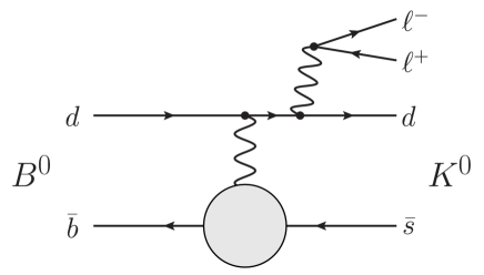
Figure 1: Feynman diagram for $B^{0}\rightarrow K^{0}\ell^{+}\ell^{-}$ due to photon emission from spectator quark.

The purpose of the present paper is to demonstrate sizable contribution of photon emission from the spectator quark rather than to propose a new mechanism of the $b$-$s$ transition. In the present model, the photon emission from the spectator quark $d$ ($u$), $d\rightarrow d+\gamma$ ($u\rightarrow u+\gamma$) is independent of the $b$-$s$ transition mechanism, and the characteristic results are due to a straightforward estimate of the quark propagator which cannot be incorporated into the factorization method. Therefore, in the present paper, to specify the origin of the $b$-$s$ transition is not essential. At present, the most likely candidate of such a $b$-$s$ transition will be the so-called gluon-penguin contribution without discrimination of spectator quarks. However, it is also interesting to consider another possibility, an exchange of a family gauge boson $A_{2}^{3}$ as shown in Fig. 2 instead of the gluon penguin. Here $A_{2}^{3}$ is a family gauge boson which changes family number from “2” to “3”. We will give a brief review of the family gauge boson model [18] in the next section (and also Appendix.A). The results for $B^{0}$ and $B^{+}$ will be highly dependent as whether we adopt family gauge boson model or gluon penguin model.

In Sec. 3, we discuss our assumptions in the effective valence quark model. In Sec. 4, we give a form factor-like function $f_{+}(q^{2})$ which gives contribution of photon emission from quarks. (However, as we emphasize in Sec. 3, the factor $f_{+}(q^{2})$ is not the so-called “form factor”. In the present prescription, we do not introduce any form factor. The factor $f_{+}(q^{2})$ originates the existence of quark propagator seen in Fig. 1.) In Sec. 4, we put an assumption in order to calculate the function $f_{+}(q^{2})$ simply. One of the purposes of the present paper is to demonstrate such $q^{2}$ dependence of the factors $f_{+}(q^{2})$ given in Eqs. (4.14) - (4.17) corresponding to four diagrams given in Fig. 3. The numerical results are given by Fig. 4 in Sec. 6. Our purpose is to see the individual contribution from each quark to the photon emission as shown in Fig. 4 (a) - (d), so that the standard model contributions are oversimplified as given in Eq. (1.3) and we do not take QCD corrections into consideration in this our naive results. Finally, Sec. 7 is devoted to the concluding remarks. Our results are somewhat different from the conventional one. The reason of the difference is in that in the present calculation we straightforwardly calculate effects of the quark propagator between the gauge-boson mediated vertex and the emitted photon vertex. We will emphasize the meaning of our prescription.

2 Another possibility of $b\rightarrow s$ transition

As we stated in Sec. 1, we demonstrate spectator effects based on a family gauge boson model. As we show in Fig. 2, the energy-momentum due to $b$-$s$ transition is transmitted to the spectator quark $d$ mediated by a family gauge boson $A_{2}^{3}$.

The family gauge boson model [18] has somewhat peculiar characteristics differently from conventional family gauge boson models. The model has the following characteristics: (i) The family symmetry is U(3) [not SU(3)], so that we have nine family gauge bosons (not eight those). (ii) The family gauge boson interactions are given by

$${\cal H}_{fam}=g_{F}\left[(\bar{e}_{i}\gamma_{\mu}e_{j})+(\bar{\nu}_{i}\gamma_{\mu}\nu_{j})+U^{*d}_{ik}U_{jl}^{d}(\bar{d}_{k}\gamma_{\mu}d_{l})+U^{*u}_{ik}U_{jl}^{u}(\bar{u}_{k}\gamma_{\mu}u_{l})\right](A_{i}^{j})^{\mu}\,.$$ (2.1)

Note that the family gauge boson mass matrix is diagonal on the basis in which the charged lepton mass matrix is diagonal, so that flavor-changing process appear only in the quark sector. (iii) $K^{0}$-$\bar{K}^{0}$, $D^{0}$-$\bar{D}^{0}$ and $B^{0}$-$\bar{B}^{0}$ mixings are caused only through non-zero quark-family mixing ($U^{u}\neq{\bf 1}$ and $U^{d}\neq{\bf 1}$). Note that if the U(3) family symmetry is broken by ${\bf 3}$ and/or ${\bf 6}$ of U(3) as a conventional family gauge boson, a direct transition $A_{i}^{j}\leftrightarrow A_{j}^{i}$ will appear, while, in the present model, there are no such scalars. For example, $B_{s}^{0}$-$\bar{B}_{s}^{0}$ mixing is only caused through the down-quark mixing $U^{d}\neq{\bf 1}$. If we suppose $U^{d}\simeq V_{CKM}$ (i.e. $U^{u}\simeq{\bf 1}$), the gauge boson contribution to the $B_{s}^{0}$-$\bar{B}_{s}^{0}$ mixing is suppressed enough by the CKM elements. (For more details, see Appendix.A.)

Such a family gauge boson model without a direct mixing $A_{i}^{j}\leftrightarrow A_{j}^{i}$ was first proposed by Sumino [21]. Therefore, the family gauge boson $A_{2}^{3}$ in the present model cannot contribute to $B_{s}$-$\bar{B}_{s}$ mixing directly. Straightforwardly speaking, the mass of $A_{2}^{3}$ is independent of constraints from these ps-meson-anti-ps-meson mixings. (iv) The gauge boson masses are given with an inverted mass hierarchy i.e. $m^{2}(A_{1}^{1}),m^{2}(A_{2}^{1}),m^{2}(A_{3}^{1})\gg m^{2}(A_{2}^{2})\gg m^{2}(A_{2}^{3})\gg m^{2}(A_{3}^{3})$, so that we may suppose a mass of $A_{2}^{3}$ of an order of $1-10$ TeV [22].

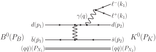
Figure 2: Feynman diagram for $B^{0}\rightarrow K^{0}\ell^{+}\ell^{-}$ and the momentum assignments.

In the present paper, for the time being, we assume the mixing matrix among up-quarks is almost unit matrix, thus its mixings are negligibly small compared with that among down-quarks. As a result, we discuss only the case of neutral B meson decay:

$$B^{0}(P_{B})\rightarrow K^{0}(P_{K})+\ell^{-}(k_{1})+\ell^{+}(k_{2})\,.$$ (2.2)

We define momenta of quarks $\bar{b}$ and $d$ inside the bottom meson $B^{0}$ as $\bar{p}_{1}$ and $p_{1}$, respectively, and $\bar{s}$ and $d$ inside $K^{0}$ as $\bar{p}_{2}$ and $p_{2}$, respectively as shown in Fig. 2. We also define the momentum of photon as $q$ in the decay $B^{0}(P_{B})\rightarrow K^{0}(P_{K})+\ell^{-}(k_{1})+\ell^{+}(k_{2})$, i.e.

$$q\equiv k_{1}+k_{2}=P_{B}-P_{K}\,.$$ (2.3)

Here, note that the momentum $P_{B}$ ($P_{K}$) is given by sum of momenta $p_{1}+\bar{p}_{1}+P_{X_{1}}$ ($p_{2}+\bar{p}_{2}+P_{X_{2}}$) of the valence quarks and sea quarks:

$$\bar{p}_{1}+p_{1}+P_{X_{1}}=P_{B}\,,\ \ \ \ \bar{p}_{2}+p_{2}+P_{X_{2}}=P_{K}\,,$$ (2.4)

where $P_{X_{1}}$ and $P_{X_{2}}$ are momenta of sea-quarks in the $B$ and $K$ mesons, respectively.

In order to know the momenta $\bar{p}_{1}$, $p_{1}$, $\bar{p}_{2}$ and $p_{2}$, we must reveal dynamical structures of the mesons. That is, in order to calculate the diagram given in Fig. 2, we solve the dynamics of the system $(B\rightarrow K)$. We integrate the diagram Fig. 2 with respect to the inner momenta $p_{1}$, $p_{2}$, $\bar{p}_{1}$, $\bar{p}_{2}$, $P_{X1}$ and $P_{X2}$, and thereby, we can obtain the matrix element in terms of the observable quantities $P_{B}$ and $P_{K}$ only. In this paper, in an effort to calculate such new type diagram, we propose an approach as a kind of the effective theory for valence quark diagrams. In the next section, we represent those momenta $\bar{p}_{1}$, $p_{1}$, $\bar{p}_{2}$ and $p_{2}$ in terms of $P_{B}$ and $P_{K}$ with the help of an “on-shell quark” assumption. Thereby, we will estimate such diagrams given in Fig. 2. Under this prescription, we will find that it is possible for photon to be emitted from $d$ quark.

3 Effective valence quark model

In the present paper, we denote momenta of $B^{0}$, $K^{0}$, $\bar{b}$ and $d$ in the $B^{0}$ meson, $s$ and $d$ in the neutral kaon $K^{0}$ as $P_{B}$, $P_{K}$, $\bar{p}_{1}$ and $p_{1}$, $\bar{p}_{2}$ and $p_{2}$, respectively. Our assumption of “on-shell quark” demands that quark masses are given by

$$\bar{p}_{1}^{2}=m_{b}^{2}\,,\ \ \ p_{1}^{2}=m_{d1}^{2}\,,\ \ \ \bar{p}_{2}^{2}=m_{s}^{2}\,,\ \ \ p_{2}^{2}=m_{d2}^{2}\,,$$ (3.1)

where we have left a possibility that the mass of the $d$ quark in the bottom meson can be different from that of the $d$ quark in the kaon, so that we have denoted those as $m_{d1}$ and $m_{d2}$, respectively. Here, it is our essential assumption that these quark masses are almost constant for $q^{2}$, although those are still dependent on the energy scale $\mu$ of the system.

If we want to calculate a meson decay into a meson and something, we must solve a composite state problem. For example, in the $\bar{b}(x_{b})$ and $d(x_{d})$ system for the $B^{0}(X)$ meson, two body bound state problem can be reduced into a one-body problem as to the relative coordinates $x=x_{b}-x_{d}$. The variables $x=x_{b}-x_{d}$ and $X_{B}=(x_{b}+x_{d})/2$ corresponds to the momenta $p_{b}-p_{d}$ [($\bar{p}_{1}-p_{1})$ in the notation in Eq. (3.1)] and $P_{B}=p_{b}+p_{d}$, respectively. However, in general, it is hard to solve such dynamics relativistically and exactly. Therefore, we usually use an easier method. For example, we can treat the system as a two-body system of quark and anti-quark system non-relativistically. Then, we must use effective quark masses (not the running quark masses $m_{q}(\mu)$) as masses of the constituents, in which all of the effects of gluons, sea-quarks, and all the rest are already taken into consideration. (For such a semi-classical approach to pseudo-scalar mesons, for example, see Ref.[23].) Another easy method is to use the running quark mass values for the valence quarks, but is to consider that the valence quarks in the meson carry only a part of the momentum of the meson. In this paper, we adopt the latter prescription.

We define the fraction parameters $x_{1}$ and $x_{2}$ as follows:

$$\bar{p}_{1}+p_{1}=P_{B}-P_{X_{1}}\equiv x_{1}P_{B}\,,\ \ \ \ \bar{p}_{2}+p_{2}=P_{K}-P_{X_{2}}\equiv x_{2}P_{K}\,,$$ (3.2)

where $x_{1}$ ($x_{2}$) is a fraction of momenta $p_{1}$ and $\bar{p}_{1}$ ($p_{2}$ and $\bar{p}_{2}$) of the valence quarks $d$ and $\bar{b}$ ($d$ and $\bar{s}$) versus the meson momentum $P_{B}$ ($P_{K}$). This is a big assumption, because Lorentz vector $\bar{p}_{1}+p_{1}$ and $P_{B}$ cannot, in general, be connected each other by Lorentz scalar $x_{1}$. The parameters $x_{1}$ and $x_{2}$ are analogous to $x$ parameters in the high energy quark parton model in which $x$ distributions of the quark partons are well known (for a review, for example, see [24]). Usually, the matrix element of $B\rightarrow K$ is obtained by integrating with respected to $x_{i}$ ($i=1,2$) over $x_{imin}\leq x_{i}\leq 1$. However, in the present prescription, for simplicity, we will substitute special values $x_{i}(q^{2}_{max})$ for $x_{i}(q^{2})$ as we show in Eqs. (3.15) and (3.16) later.

From the constraint (3.2), we have the following relations

$$x_{1}^{2}M_{B}^{2}+m_{d1}^{2}-2x_{1}(p_{1}P_{B})=m_{b}^{2}\,,\ \ \ \ x_{2}^{2}M_{K}^{2}+m_{d2}^{2}-2x_{2}(p_{2}P_{K})=m_{s}^{2}\,.$$ (3.3)

Under the on-shell assumption, the quark momenta $p_{1}$ and $p_{2}$ can be expressed in terms of $P_{B}$ and $P_{K}$:

$$\begin{split}p_{1}^{\mu}&=a_{1}(P_{B}+P_{K})^{\mu}+b_{1}(P_{B}-P_{K})^{\mu}\,,\\ p_{2}^{\mu}&=a_{2}(P_{B}+P_{K})^{\mu}+b_{2}(P_{K}-P_{B})^{\mu}\,,\end{split}$$ (3.4)

where the coefficients $a_{1}$, $b_{1}$, $a_{2}$ and $b_{2}$ can, in general, be functions of $q^{2}$. [This is also a big assumption in this formulation. Note that we put this assumption only on momenta $(p_{1},p_{2})$, but not on $(\bar{p}_{1},\bar{p}_{2})$ and $(P_{X1},P_{X2})$, correspondingly to Fig. 2.] Then, we can obtain relations

$$m_{d1}^{2} = a_{1}^{2}[2(M_{B}^{2}+M_{K}^{2})-q^{2}]+b_{1}^{2}\,q^{2}+2a_{1}b_{1}\Delta_{BK}^{2}\,,$$ (3.5)

$$m_{d2}^{2} = a_{2}^{2}[2(M_{B}^{2}+M_{K}^{2})-q^{2}]+b_{2}^{2}\,q^{2}-2a_{2}b_{2}\Delta_{BK}^{2}\,,$$ (3.6)

from Eq. (3.1), and

$$x_{1}^{2}M_{B}^{2}+m_{d1}^{2}-m_{b}^{2} = x_{1}a_{1}\left[2(M_{B}^{2}+M_{K}^{2})+\Delta_{BK}^{2}-q^{2}\right]+x_{1}b_{1}\left(\Delta_{BK}^{2}+q^{2}\right)\,,$$ (3.7)

$$x_{2}^{2}M_{K}^{2}+m_{d2}^{2}-m_{s}^{2} = x_{2}a_{2}\left[2(M_{B}^{2}+M_{K}^{2})-\Delta_{BK}^{2}-q^{2}\right]+x_{2}b_{2}\left(-\Delta_{BK}^{2}+q^{2}\right)\,,$$ (3.8)

from Eq. (3.4), where

$$\Delta_{BK}^{2}\equiv M_{B}^{2}-M_{K}^{2}\,.$$ (3.9)

Thus, if we give values of $x_{1}$ and $x_{2}$, we can completely determine the coefficients $(a_{1},b_{1})$ from the two relations (3.5) and (3.7), and $(a_{2},b_{2})$ from the two relations (3.6) and (3.8), respectively. Here, note that the replacement $(M_{B},m_{b},m_{d1})\rightarrow(M_{K},m_{s},m_{d2})$ gives $(a_{1},b_{1})\rightarrow(a_{2},b_{2})$. Therefore, hereafter, we will discuss the relations only on $(a_{1},b_{1})$.

The coefficients $(a_{1},b_{1})$ can be obtained as follows. From Eq. (3.5), we obtain a relation between $a_{1}$ and $b_{1}$ (see Appendix.D):

$$b_{1}=\frac{1}{q^{2}}\left[-a_{1}\Delta_{BK}^{2}\pm\sqrt{Da_{1}^{2}+m_{d1}^{2}q^{2}}\right]\,,$$ (3.10)

where

$$D=\left[(M_{B}-M_{K})^{2}-q^{2}\right]\left[(M_{B}+M_{K})^{2}-q^{2}\right]\,.$$ (3.11)

By substituting Eq. (3.10) into Eq. (3.5), we obtain a relation for $a_{1}$

$$x_{1}^{2}M_{B}^{2}+m_{d1}^{2}-m_{b}^{2}=\frac{x_{1}}{q^{2}}\left[-a_{1}D\pm(\Delta_{BK}^{2}+q^{2})\sqrt{a_{1}^{2}D+m_{d1}^{2}q^{2}}\right]\,.$$ (3.12)

The parameter $a_{1}$ can be obtained by solving Eq. (3.12) for $a_{1}$.

The relation (3.12) brings a new constraint to the model: Let us consider a limit of $q^{2}=q^{2}_{max}$, where

$$q^{2}_{max}\equiv(M_{B}-M_{K})^{2}\,,$$ (3.13)

and it gives

$$D(q^{2})|_{q^{2}=q^{2}_{max}}=0\,.$$ (3.14)

Therefore, the relation (3.12) at a limit of $q^{2}=q^{2}_{max}$ leads to a constraint

$$x_{1}M_{B}=m_{b}\pm m_{d1}\,.$$ (3.15)

Note that the parameter $x_{1}$ in the definition (3.2) was dependent on the inner momentum $P_{X1}$ (i.e. $\bar{p}_{1}+p_{1}$), while $x_{1}$ given in (3.15) is a constant (although the value $x_{1}$ given in (3.15) is still dependent on the energy scale $\mu$). The crucial assumption is that we can approximately use the value of $x_{1}(q^{2}_{max})$ instead of $x_{1}(q^{2})$ for whole physical region $q^{2}_{min}\leq q^{2}\leq q^{2}_{max}$.

Similarly, we obtain a constraint

$$x_{2}M_{K}=m_{s}\pm m_{d2}\,.$$ (3.16)

Note that the sign $\pm$ in Eq. (3.15) corresponds to the sign $\pm$ in the relation (3.12), but the sign $\pm$ in Eq. (3.15) and $\pm$ in Eq. (3.16) are independent each other.

Quark masses $m_{b}$, $m_{s}$ and $m_{d}$ are function of the energy scale $\mu$, but it does not mean that those are always function of $q^{2}$ directly. We consider that the quark mass values $m_{b}$, $m_{s}$ and $m_{d}$ in the $B\rightarrow K\ell^{+}\ell^{-}$ decays are described by those at $\mu\sim M_{B}$. Then, we can estimate the values of $x_{1}$ and $x_{2}$ from Eqs. (3.15) and (3.16), so that we can also estimate the values of $(a_{1},b_{1})$ and $(a_{2},b_{2})$.

More discussions from a phenomenological point of view will be given in Sec. 4.

4 $\ell^{+}\ell^{-}$ emission from valence quark: $q\rightarrow q+\gamma$ vs $\bar{b}\rightarrow\bar{s}+\gamma$ in $B=(q\bar{b})$

We assume the following interactions for $B\rightarrow K\ell^{+}\ell^{-}$ in addition to the conventional $b\rightarrow s+\gamma$ interaction (1.1):

$${\cal H}=\sum_{q=u,d,b,s}e_{q}(\bar{q}\gamma_{\mu}q)A^{\mu}-\sum_{\ell=e,\mu}e(\bar{\ell}\gamma_{\mu}\ell)A^{\mu}+\sum_{q=u,d}G_{fam}^{q}(\bar{b}\gamma_{\rho}s)(\bar{q}\gamma^{\rho}q)\,,$$ (4.1)

where $e_{d}=e_{s}=e_{b}=-e/3$, $e_{u}=2e/3$, and

$$G_{fam}^{q}=\frac{g_{F}^{2}}{M_{23}^{2}}U_{33}^{\ast d}U_{22}^{d}U_{21}^{\ast q}U_{31}^{q}\,.$$ (4.2)

Here, $U_{ij}^{q}$ are mixing matrix elements among quarks $q=(q_{1},q_{2},q_{3})$, and $M_{23}$ is a mass of a family gauge boson $A_{2}^{3}$. Based on the interactions (4.1), we calculate the following four diagrams for $B^{0}\rightarrow K^{0}\ell^{+}\ell^{-}$ as shown in Fig. 3. Calculations corresponding to Fig. 3 (a) - (d) based on the standard model have already been given, for example, in Ref.[25]. In our prescription, especially, a role of the propagator in Fig. 3 (quark-line which is not connected directly to the mesons $B$ and $K$) is investigated.

Hereafter, since we are interested in a case $B^{0}\rightarrow K^{0}\ell^{+}\ell^{-}$, we will calculate only the case. Another case $B^{+}\rightarrow K^{+}\ell^{+}\ell^{-}$ can easily be obtained by replacing $e_{d}\rightarrow e_{u}$ and $U^{d}\rightarrow U^{u}$.

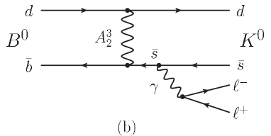
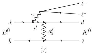
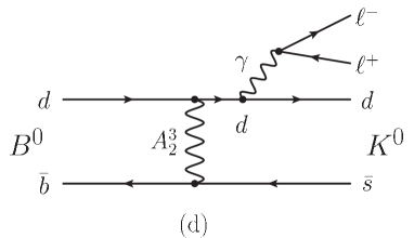
Figure 3: Feynman diagrams for $B^{0}\rightarrow K^{0}\ell^{+}\ell^{-}$.

Denominators of the propagators with momenta $\ell$ shown in Figs. 3 (a), (b), (c) and (d) are given as follows:

$$\Delta_{a} \equiv \ell_{(a)}^{2}-m_{b}^{2}=q^{2}-2\bar{p}_{1}q\,,$$ (4.3)

$$\Delta_{b} \equiv \ell_{(b)}^{2}-m_{s}^{2}=q^{2}+2\bar{p}_{2}q\,,$$ (4.4)

$$\Delta_{c} \equiv \ell_{(c)}^{2}-m_{d1}^{2}=q^{2}-2{p}_{1}q\,,$$ (4.5)

$$\Delta_{d} \equiv \ell_{(d)}^{2}-m_{d2}^{2}=q^{2}+2{p}_{2}q\,.$$ (4.6)

By using the coefficients defined by Eq. (3.4), the expressions (4.3) - (4.6) are rewritten as follows:

$$\Delta_{a} = (2a_{1}-x_{1})\Delta_{BK}^{2}+(1-x_{1}+2b_{1})q^{2}\,,$$ (4.7)

$$\Delta_{b} = -(2a_{2}-x_{2})\Delta_{BK}^{2}+(1-x_{2}+2b_{2})q^{2}\,,$$ (4.8)

$$\Delta_{c} = -2a_{1}\Delta_{BK}^{2}+(1-2b_{1})q^{2}\,,$$ (4.9)

$$\Delta_{d} = 2a_{2}\Delta_{BK}^{2}+(1-2b_{2})q^{2}\,.$$ (4.10)

In order to translate effective interactions among quarks into hadronic fields, we use

$$\langle 0|(\bar{b}\gamma^{\mu}\gamma_{5}d)|B^{0}(P_{B})\rangle=-iP^{\mu}_{B}f_{B}\,,$$ (4.11)

for the initial state and apply same approach to the final state. The details to obtain amplitudes which correspond to the diagrams (a), (b), (c) and (d) in Fig. 3 are given in Appendix.B.

When we use the expression (3.4), we obtain the following form for the meson currents:

$${\cal M}=i\frac{1}{6}\bar{e}_{b}ef_{K}f_{B}G_{fam}\frac{1}{2}\left[f_{+}(q^{2})(P_{B}+P_{K})_{\mu}+f_{-}(q^{2})(P_{B}-P_{K})_{\mu}\right]\frac{1}{q^{2}}[\bar{v}_{\ell}(k_{2})\gamma^{\mu}u_{\ell}(k_{1})]\,,$$ (4.12)

where $G_{fam}$ is defined by Eq. (4.2) and we have dropped the index $q=d$ because it is obvious that we calculate a case of $B^{0}\rightarrow K^{0}\ell^{+}\ell^{-}$.

The second term with $q_{\mu}=(P_{B}-P_{K})_{\mu}$ in Eq. (4.12) does not contribute the decay amplitudes because of $q_{\mu}[\bar{v}_{\ell}(k_{2})\gamma^{\mu}u_{\ell}(k_{1})]=0$ for $m_{\ell 1}=m_{\ell 2}$. For the expression $f_{+}(q^{2})$, we obtain

$$f_{+}(q^{2})=f_{+}^{a}(q^{2})+f_{+}^{b}(q^{2})-f_{+}^{c}(q^{2})-f_{+}^{d}(q^{2})\,,$$ (4.13)

where

$$f_{+}^{a}(q^{2}) = \frac{(x_{1}-2a_{1})M_{K}^{2}+(1-x_{1}+a_{1}+b_{1})q^{2}}{-(x_{1}-2a_{1})\Delta_{BK}^{2}+(1-x_{1}+2b_{1})q^{2}}\,,$$ (4.14)

$$f_{+}^{b}(q^{2}) = \frac{(x_{2}-2a_{2})M_{B}^{2}+(1-x_{2}+a_{2}+b_{2})q^{2}}{(x_{2}-2a_{2})\Delta_{BK}^{2}+(1-x_{2}+2b_{2})q^{2}}\,,$$ (4.15)

$$f_{+}^{c}(q^{2}) = \frac{2a_{1}M_{K}^{2}+(1-a_{1}-b_{1})q^{2}}{-2a_{1}\Delta_{BK}^{2}+(1-2b_{1})q^{2}}\,,$$ (4.16)

$$f_{+}^{d}(q^{2}) = \frac{2a_{2}M_{B}^{2}+(1-a_{2}-b_{2})q^{2}}{2a_{2}\Delta_{BK}^{2}+(1-2b_{2})q^{2}}\,.$$ (4.17)

Note that these factors $f_{+}(q^{2})$ given in Eqs. (4.14) - (4.17) are not the so-called “form factor” which denotes a quark structure. The functions, $f_{+}^{a}(q^{2})$, $f_{+}^{b}(q^{2})$, $f_{+}^{c}(q^{2})$ and $f_{+}^{d}(q^{2})$, originate in the propagators shown in Fig. 3 (a) - (d). Although we do not introduce any form factor since it is not a main story in the present prescription, this does not mean that we deny the existence of such form factors. It will become important to take such effects into consideration in an extended study in a future.

So far we have discussed the case of the decay mode $B^{0}\rightarrow K^{0}\ell^{+}\ell^{-}$, because we have considered that up-quark mixing will be considerably small compared with down-quark mixing, $|U^{u}_{ij}|^{2}\ll|U^{d}_{ij}|^{2}$. However, we can easily calculate the case $B^{+}\rightarrow K^{+}\ell^{+}\ell^{-}$ similarly to the case $B^{0}\rightarrow K^{0}\ell^{+}\ell^{-}$: A form of $f_{+}(q^{2})$ for the decay $B^{+}\rightarrow K^{+}\ell^{+}\ell^{-}$ can be obtained by replacing $e_{d}=-e/3\rightarrow e_{u}=+2e/3$ in Eq. (4.13), i.e.

$$f_{+}(q^{2})=f_{+}^{a}(q^{2})+f_{+}^{b}(q^{2})+2f_{+}^{c}(q^{2})+2f_{+}^{d}(q^{2})\,.$$ (4.18)

5 Interference effect in $d\Gamma/dq^{2}$

The partial decay width $\Gamma(B\rightarrow K\ell^{+}\ell^{-})$ is calculated from the matrix element

$${\cal M}=G\left(1+\xi\frac{f_{+}(q^{2})}{q^{2}}\right)(P_{B}+P_{K})_{\mu}[\bar{v}_{\ell}(k_{2})\gamma^{\mu}u_{\ell}(k_{1})]\,,$$ (5.1)

where

$$G=G^{eff}_{EW}\frac{2m_{b}f_{T}(0)}{M_{B}+M_{K}}\,.$$ (5.2)

Here, for simplicity, we have neglected the $q^{2}$ dependence of the form factor $f_{T}(q^{2})$ in the conventional model. (The numerical results are not almost change even if we take the $q^{2}$ dependence of $f_{T}(q^{2})$ into consideration. We will demonstrate it in Appendix.E.) The parameter $\xi$ is defined by

$$\xi=\frac{g_{fam}^{2}}{g_{w}^{2}}\frac{8M_{w}^{2}}{M_{23}^{2}}\frac{U_{33}^{\ast d}U_{22}^{d}U_{21}^{\ast d}U_{31}^{d}}{V_{ts}^{*}V_{tb}}\frac{\pi^{2}}{9}\frac{M_{B}+M_{K}}{2m_{b}f_{T}(0)}f_{K}f_{B}\,.$$ (5.3)

Certainly, this parameter should be $\left|\xi\right|\sim 10^{-5}{\rm GeV}^{2}$ with $M_{23}\sim$ a few TeV at a rough estimation in the family gauge boson model. But, at present, we regard this parameter $\xi$ as a free parameter whose value is phenomenologically determined by the observed $q^{2}$ dependence of $dBr/dq^{2}$. Let us define a function $F(q^{2})$ as

$$G^{2}F(q^{2})\equiv\left.\frac{d\Gamma}{dq^{2}}\right|_{\xi=0}=\frac{1}{(2\pi)^{3}}\frac{1}{32M_{B}^{3}}\int_{y_{1}}^{y_{2}}dy\,|{\cal M}|^{2}_{\xi=0}\,,$$ (5.4)

where $y\equiv m^{2}_{\ell K}=(k_{2}+P_{K})^{2}$, and $y_{1}=y_{min}$, $y_{2}=y_{max}$. Then, $d\Gamma/dq^{2}$ is given by

$$\frac{d\Gamma}{dq^{2}}(B\rightarrow K\ell^{+}\ell^{-})=G^{2}\left(1+\xi\frac{f_{+}(q^{2})}{q^{2}}\right)^{2}F(q^{2})\,.$$ (5.5)

The explicit form of $F(q^{2})$ is appeared in Appendix.C.

Now, we can numerically evaluate the function $f_{+}(q^{2})$ and ${d\Gamma}/{dq^{2}}$ by using these formulas (5.1) - (5.5). First, we give quark mass values $m_{b}(\mu)$, $m_{s}(\mu)$, and $m_{d1}(\mu)=m_{d2}(\mu)$ at $\mu=M_{B}-M_{K}$. Then, we obtain the values, $x_{1}$ and $x_{2}$, by the relations (3.15) and (3.16). We assume that the quark mass values in this prescription are almost independent of $q^{2}$, and those are only dependent on the value $\mu$. We assume that these quark masses at $\mu=M_{B}-M_{K}$ are approximately not so deviated from those at $\mu=M_{B}$, so that we use the values which are determined by using (3.15) and (3.16). The coefficients $a_{1}$ ($a_{2}$) can be obtained by using Eq. (3.12) and then $a_{1}$ ($a_{2}$) can be gotten by using Eq. (3.10). We will obtain two solutions for Eq. (3.12). Note that the coefficients $(a_{1},b_{1})$ and $(a_{2},b_{2})$ are, in general, given as functions of $q^{2}$.

However, in order to give a more concise form of $(a_{1},b_{1})$ and $(a_{2},b_{2})$, let us put the following assumption from phenomenological point of view: These coefficients have no $q^{2}$ dependence approximately. This demands $a_{1}=b_{1}$ ($a_{2}=b_{2}$) as seen in Eqs. (3.5) and (3.7) [Eqs. (3.6) and (3.8)]. Then, we obtain concise forms

$$a_{1}=b_{1}=\pm\frac{m_{d1}}{2M_{B}}\,,\ \ \ a_{2}=b_{2}=\pm\frac{m_{d2}}{2M_{K}}\,,$$ (5.6)

from Eq. (3.12). The sign $\pm$ in (5.6) corresponds to $\pm$ in Eq. (3.12), but the sign $\pm$ in $a_{1}=b_{1}$ need not to correspond to that in $a_{2}=b_{2}$. By using these solutions in Eq. (5.6), the expressions (4.14) - (4.17) are rewritten as follows:

$$f_{+}^{a}(q^{2}) = \frac{m_{b}M_{K}^{2}+(M_{B}-m_{b})q^{2}}{-m_{b}\Delta_{BK}^{2}+(M_{B}-m_{b})q^{2}}\,,$$ (5.7)

$$f_{+}^{b}(q^{2}) = \frac{m_{s}M_{B}^{2}+(M_{K}-m_{s})q^{2}}{m_{s}\Delta_{BK}^{2}+(M_{K}-m_{s})q^{2}}\,,$$ (5.8)

$$f_{+}^{c}(q^{2}) = \frac{\pm m_{d1}M_{K}^{2}+(M_{B}\mp m_{d1})q^{2}}{\mp m_{d1}\Delta_{BK}^{2}+(M_{B}\mp m_{d1})q^{2}}\,,$$ (5.9)

$$f_{+}^{d}(q^{2}) = \frac{\pm m_{d2}M_{B}^{2}+(M_{K}\mp m_{d2})q^{2}}{\pm m_{d2}\Delta_{BK}^{2}+(M_{K}\mp m_{d2})q^{2}}\,.$$ (5.10)

Note that $f_{+}^{a}(q^{2})$ and $f_{+}^{b}(q^{2})$ are independent of the choices $\pm$ in Eq. (5.6), but $f_{+}^{c}(q^{2})$ and $f_{+}^{d}(q^{2})$ are dependent on the choices. If we take the positive sign for $a_{1}=b_{1}$ in (5.6), then the function $f_{+}^{c}(q^{2})$ will have a pole at $q^{2}=m_{d1}\Delta_{BK}^{2}/(M_{B}-m_{d1})$. Also, if we take the negative sign in Eq. (5.6), then the function $f_{+}^{d}(q^{2})$ will have a pole at $q^{2}=m_{d2}\Delta_{BK}^{2}/(M_{K}+m_{d2})$. Therefore, in the numerical estimate of $d\Gamma/dq^{2}$, we take the signs in Eq. (5.6) as follows:

$$a_{1}=b_{1}=-\frac{m_{d1}}{2M_{B}}\,,\ \ \ a_{2}=b_{2}=+\frac{m_{d2}}{2M_{K}}\,.$$ (5.11)

Then, the propagator effects at $q^{2}=0$ are given by

$$f_{+}^{a}(0)=f_{+}^{c}(0)=-\frac{M_{K}^{2}}{M_{B}^{2}-M_{K}^{2}}\,,\ \ \ f_{+}^{b}(0)=f_{+}^{d}(0)=+\frac{M_{B}^{2}}{M_{B}^{2}-M_{K}^{2}}\,.$$ (5.12)

6 Numerical results

For numerical estimates, for convenience, we adopt quark mass values [26] at $\mu=m(m_{b})=4.34$ GeV in place of those at $\mu=M_{B}-M_{K}$:

$$m_{b}=4.34\ {\rm GeV}\,,\ \ \ m_{s}=0.127\ {\rm GeV}\,,\ \ \ m_{d}\equiv m_{d1}=m_{d2}=0.00637\ {\rm GeV}\,.$$ (6.1)

The input values (6.1) lead to the following values of the fraction factors $x_{1}$ and $x_{2}$:

$$x_{1}(B)=0.821,\ \ \ \ x_{2}(K)=0.244\,,$$ (6.2)

from Eqs. (3.15) and (3.16), respectively. We may have another choice. However, numerical results are almost similar. Hereafter, we use the values (6.1) as typical values in our prescription.

The values (6.2) mean that the valence quarks $b$ and $d$ are almost dominant in the $B$ meson, while the valence quarks $s$ and $d$ carry only 24% of the momentum of the kaon in the final state. However, the value $x_{2}(K)=0.244$ is not common in the all kaon processes, but the value $x_{2}(K)=0.244$ is one only in the case of $B\rightarrow K\ell^{+}\ell^{-}$. For example, in a kaon decay (note that the value is not $x_{2}$, but it is $x_{1}$ because $K$ is one in the initial state), we will again obtain a value close to $x_{1}(K)\simeq 1$, because in this times we will use quark mass values $m_{s}(\mu)$ and $m_{d}(\mu)$ at $\mu=M_{K}$ (not $\mu=M_{B}$).

(a) $f_{+}^{a}(q^{2})$                                                          (b) $f_{+}^{b}(q^{2})$

(c) $f_{+}^{c}(q^{2})$                                                          (d) $f_{+}^{d}(q^{2})$

Figure 4: Contribution from each quark line to the functions $f_{+}(q^{2})$. Figures are illustrated for a physical range $4m_{\mu}^{2}<q^{2}<(M_{B}-M_{K})^{2}$.

First, in Fig. 4, we show the behavior of the functions $f_{+}^{a}(q^{2})$, $f_{+}^{b}(q^{2})$, $f_{+}^{c}(q^{2})$ and $f_{+}^{d}(q^{2})$ which represent the contributions of photon emissions from $b$, $s$, $d_{1}$ and $d_{2}$ quarks, respectively, and which are due to quark propagator effects. Note that although we have chosen the coefficients $(a_{1},b_{1})$ and $(a_{2},b_{2})$ so that those are independent of $q^{2}$, the functions $f_{+}^{a}(q^{2})$, $f_{+}^{b}(q^{2})$, $f_{+}^{c}(q^{2})$ and $f_{+}^{d}(q^{2})$ still depend on $q^{2}$. We find that $f_{+}^{b}(q^{2})\simeq+1$ and $f_{+}^{d}(q^{2})\simeq+1$ for whole range of $q^{2}$, and $f_{+}^{c}(q^{2})\simeq+1$ except for a small range of $q^{2}$. Also, we show the behavior of $f_{+}(q^{2})$ in Fig. 5. Note that $f_{+}(q^{2})<0$ over the whole physical region.

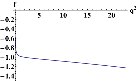
Figure 5: Behavior of $f_{+}(q^{2})$ in the neutral B meson decay $B^{0}\rightarrow K^{0}\ell^{+}\ell^{-}$.

Also, we show the behavior of $dBr(B^{0}\rightarrow K^{0}\ell^{+}\ell^{-})/dq^{2}$ in the unit of $G^{2}$ defined by Eq. (5.2) for typical values of the parameter $\xi$ in Fig. 6. We can obtain a reasonable dip at $q^{2}\sim 1$ GeV with $\xi=0.6$.

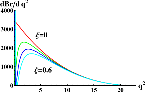
Figure 6: Behavior of $dBr/dq^{2}$ in the decay $B^{0}\rightarrow K^{0}\ell^{+}\ell^{-}$ in the unit of $G^{2}$ defined by Eq. (5.2). Curves are lined up in order of the cases $\xi=0$, $0.2$, $0.4$ and $0.6$ in the unit of GeV² (the colors red, green, blue and cyan, respectively).

Similarly, we can demonstrate the case of $B^{+}\rightarrow K^{+}\ell^{+}\ell^{-}$. The behaviors of $f_{+}(q^{2})$ and $dBr/dq^{2}$ are illustrated in Figs. 7 and 8, respectively. (Here, for convenience, we have used the same value of $G$ defined by Eq. (5.2), although a weak annihilation diagram effect [17] should be added in the case of $B^{+}\rightarrow K^{+}\ell^{+}\ell^{-}$.) If the up-quark mixing is sizable compared with the down-quark mixing, the case will be also visible. The shape of the $dBr/dq^{2}$ in $B^{+}\rightarrow K^{+}\ell^{+}\ell^{-}$ is almost similar to that in $B^{0}\rightarrow K^{0}\ell^{+}\ell^{-}$. However, note that the dip in $dBr/dq^{2}$ appears for $\xi>0$ in the case $B^{0}\rightarrow K^{0}\ell^{+}\ell^{-}$, while the dip appears for $\xi<0$ in the case $B^{+}\rightarrow K^{+}\ell^{+}\ell^{-}$. It will be possible because $U^{\ast u}_{21}U^{u}_{31}$ takes an opposite sign to $U^{\ast d}_{21}U^{d}_{31}$. Moreover, the position of the dip is slightly shifted to the larger value of $q^{2}$ than the case of neutral B meson.

However, we do not consider that the magnitude of $U^{\ast u}_{21}U^{u}_{31}$ is accidentally the same as that of $U^{\ast d}_{21}U^{d}_{31}$. We expect that the behavior of $dBr/dq^{2}$ in $B^{+}\rightarrow K^{+}\ell^{+}\ell^{-}$ will be different from that in $B^{0}\rightarrow K^{0}\ell^{+}\ell^{-}$. We hope data of $dBr/dq^{2}$ will be able to distinguish between $B^{0}\rightarrow K^{0}\ell^{+}\ell^{-}$ and $B^{+}\rightarrow K^{+}\ell^{+}\ell^{-}$.

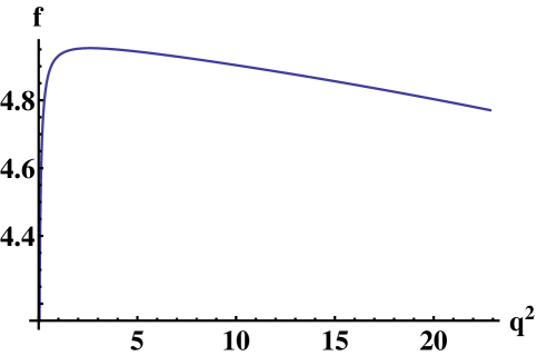
Figure 7: Behavior of $f_{+}(q^{2})$ in the charged B meson decay $B^{+}\rightarrow K^{+}\ell^{+}\ell^{-}$.

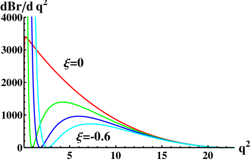
Figure 8: Behavior of $dBr/dq^{2}$ in the decay $B^{+}\rightarrow K^{+}\ell^{+}\ell^{-}$ in the unit of $G^{2}$ defined by Eq. (5.2). Curves are lined up in order of the cases $\xi=0$, $-0.2$, $-0.4$ and $-0.6$ in the unit of GeV² (the colors red, green, blue and cyan, respectively).

Finally, we would like to give some comments on the predicted partial decay width. The decay width is given by

$$\Gamma(B\rightarrow K\ell^{+}\ell^{-})=G^{2}\int_{q^{2}_{min}}^{q^{2}_{max}}dq^{2}F(q^{2})\,,$$ (6.3)

where the function $F(q^{2})$ is defined by Eq. (5.4) and $q^{2}_{min}$ is given by $q^{2}_{min}=4m_{\ell}^{2}$. The numerical value is highly sensitive to whether $\ell=\mu$ or $\ell=e$, because the contribution becomes very large at $q^{2}\simeq 0$. However, it seems to be impossible to measure accurately until $q^{2}=4m_{e}^{2}=1.044\times 10^{-6}$ GeV². If we take $q^{2}_{min}=4m_{\mu}^{2}=0.04465$ GeV² for the case of $\Gamma(B\rightarrow Ke^{+}e^{-})$, too, we cannot find a significant difference between $\Gamma(B\rightarrow Ke^{+}e^{-})$ and $\Gamma(B\rightarrow K\mu^{+}\mu^{-})$. Another comment is as follows: The predicted decay width $\Gamma(B\rightarrow K\ell^{+}\ell^{-})$ is dependent on the value of $\xi$. We illustrate the behavior $R(\xi)\equiv\Gamma(\xi)/\Gamma(0)$ in Fig. 9. The present data [27] show $Br(B^{+}\rightarrow K^{+}\ell^{+}\ell^{-})=(5.1\pm 0.5)\times 10^{-7}$, $Br(B^{0}\rightarrow K^{0}\ell^{+}\ell^{-})=(3.1^{+0.8}_{-0.7})\times 10^{-7}$ and $\tau(B^{+})/\tau(B^{0})=1.079\pm 0.007$, so that we obtain

$$R_{+/0}\equiv\frac{\Gamma(B^{+}\rightarrow K^{+}\ell^{+}\ell^{-})}{\Gamma(B^{0}\rightarrow K^{0}\ell^{+}\ell^{-})}=1.52^{+0.42}_{-0.38}\,.$$ (6.4)

Although the value has a large error, if we dare to take the center value in (5.3), a case of the value of $\xi$ which gives $R_{+/0}\sim 1.5$ is only in the case $B^{+}\rightarrow K^{+}\ell^{+}\ell^{-}$. The case with $\xi\sim 0.4$ GeV² can also give a reasonable shape of $d\Gamma/dq^{2}$ as seen in Fig. 8. However, this view conflicts with our anticipation that $|U^{\ast u}_{21}U^{u}_{31}|\ll|U^{\ast d}_{21}U^{d}_{31}|$. We must wait individual future data of $B^{0}\rightarrow K^{0}\ell^{+}\ell^{-}$ and $B^{+}\rightarrow K^{+}\ell^{+}\ell^{-}$.

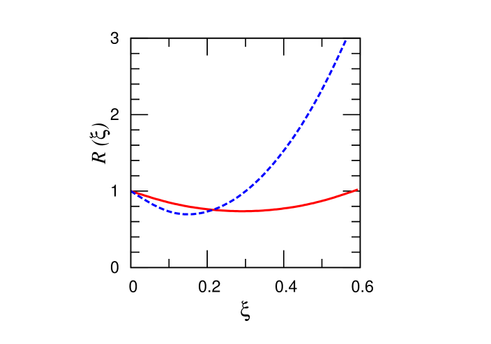
Figure 9: Behaviors of $R(\xi)\equiv\Gamma(\xi)/\Gamma(0)$ in the decays $B^{0}\rightarrow K^{0}\ell^{+}\ell^{-}$ (solid curve) and $B^{+}\rightarrow K^{+}\ell^{+}\ell^{-}$ (dashed curve).

7 Concluding remarks

In conclusion, we have investigated a contribution of photon emission from the “spectator” quark $d\rightarrow d+\gamma$ ($u\rightarrow u+\gamma$) in the $B^{0}$ ($B^{+}$) meson, and thereby we have obtained interesting results: (i) The contribution from the spectator quark is not so negligible, i.e. $f_{+}^{c}(q^{2})\simeq 1$ and $f_{+}^{d}(q^{2})\simeq 1$ in contrast to the contribution from $\bar{b}$ quark, $f_{+}^{a}(q^{2})\sim-0.1$, and that from $\bar{s}$ quark, $f_{+}^{b}(q^{2})\simeq 1$. (ii) For a sizable value of the parameter $|\xi|$, we can demonstrate a dip of $Br(B\rightarrow K\ell^{+}\ell^{-})$ in the small $q^{2}$ region. However, in order to obtain such a dip in both decay modes, $B^{0}\rightarrow K^{0}\ell^{+}\ell^{-}$ and $B^{+}\rightarrow K^{+}\ell^{+}\ell^{-}$, simultaneously, the sign of $\xi$ parameter must be opposite each other.

However, note that it is hard to compare the expression (1.3) with the prediction of the decay $B\rightarrow K\ell^{+}\ell^{-}$ from the standard model directly. Nevertheless the results $f_{+}(q^{2})$ given in Fig. 4 are independent of the form $F(q^{2})$ defined by Eq. (5.4). Actually, the $q^{2}$ dependence of $dBr/dq^{2}$ is correlated with the form $F(q^{2})$, but in the present analysis, we have not taken QCD corrections, for example form factor effects, in order to demonstrate photon emission from the spectator quark straightforwardly. Therefore, correspondingly to the treatments, we also simplify the conventional standard model contributions, too. The purpose of the present paper is to indicate the spectator quark effects qualitatively, and not to estimate the spectator quark effects quantitatively. In the numerical analysis, since our interest is the difference between $dBr(B^{0}\rightarrow K^{0}\ell^{+}\ell^{-})/dq^{2}$ and $dBr(B^{+}\rightarrow K^{+}\ell^{+}\ell^{-})/dq^{2}$, for simplicity, we have neglected some important effects. For example, we have regarded the form factor $f_{T}(q^{2})$ as a constant in respect to $q^{2}$. Therefore, the numerical results should be rigidly taken. However, we consider that the qualitative conclusions are reliable since we have treated only relative quantities (e.g. the ratios).

In the present paper, the origin of $b$-$s$ transition is not specified, although, for convenience, the formulation has been given for the case of a family gauge boson $A_{2}^{3}$ exchange. In the present paper, the $b$-$s$ transition is given in the Eq. (4.1), but the definition (4.2) of the coupling constant $G^{q}_{fam}$ is nothing but an example. The parameter $\xi$ given in Eq. (5.3) is a phenomenological one, at present. The value of $\xi$ has been treated as one which should be determined by experiments.

If we consider that the origin is due to the exchange of $A_{2}^{3}$ for example, the rough estimate of $|\xi|$ from Eq. (5.3) gives $|\xi|\sim 10^{-5}$ GeV² for $M_{23}\sim$ a few TeV. Accordingly, such contribution cannot become visible in the family gauge boson model even if it is inverted mass hierarchy [18] (also in a revised model [22]). We need some enhancement mechanism of the $A_{2}^{3}$ exchange diagrams or some other dynamics in such rare B meson decay.

On the other hand, we have other diagrams for the source of $b$-$s$ transition, electroweak penguin, gluon penguin, and other considerable processes. Especially, so far, the gluon penguin has been neglected in the operator expansion approach. If we replace the family gauge boson $A_{2}^{3}$ with gluon $g$ from the gluon penguin, the value of $\xi$ can be sizable. Therefore, we may rather regard the parameter $\xi$ defined by Eq. (5.1) as a phenomenological one, discarding Eq. (5.3). Then, the squared mass $M_{23}^{2}$ in Eq. (4.2) must be replaced with $\bar{q}^{2}=(\bar{p}_{1}-\bar{p}_{2})^{2}$. The value $\bar{q}^{2}$ is calculable in the present prescription. Since our parameters $a_{1}$, $b_{1}$, $a_{2}$ and $b_{2}$ are small, the value $\bar{q}^{2}$ is the order of $q^{2}$. Therefore, the $q^{2}$ dependence will be somewhat different from the present result based on the $A_{2}^{3}$ exchange.

In the case of gluon penguin, the decay widths of $B^{0}$ and $B^{+}$ decays are given by the same forms except for the factors $f_{+}(q^{2})$. Since the parameters $\xi(B^{0})$ and $\xi(B^{+})$ are also given by the same value, the dip in $d\Gamma/dq^{2}$ can appear only in either $B^{0}$ or $B^{+}$ decay. (For the case of $A_{2}^{3}$ exchange, $\xi(B^{0})$ and $\xi(B^{+})$ can take opposite sign each other by supposing $U^{\ast u}_{21}U^{u}_{31}/U^{\ast d}_{21}U^{d}_{31}<0$.) At present, the data by Belle [1] and BABAR [2] have shown a possibility that there is a dip in $d\Gamma/dq^{2}$, but data are not separated between $B^{0}$ and $B^{+}$. In the LHCb, we can see a possibility of a dip in the $B^{0}$ decay [3], but we cannot see such a dip in the $B^{+}$ decay [4]. It seems that this is favor of the gluon penguin model.

Thus, it is our greatest concern whether the data show a dip in $dBr/dq^{2}$ both or either in $B^{0}$ and/or $B^{+}$ decays. As in Fig. 9, we can find a possibility of appearance for isospin asymmetry, that is the difference between $B^{0}$ and $B^{+}$. In the evaluation of that figure, the overall factors should be canceled out because we have taken a ratio of the decay rate. Therefore the phenomenon of photon emission from spectator quarks itself is important to observe isospin asymmetry. We expect that such data will soon be reported.

The present results highly depend on our treatment for the quark-anti-quark bound system. In our prescription, the existence of the quark propagator, which cannot be incorporated into the factorization method, has played an essential role. We have straightforwardly and faithfully calculated the effects based on the effective valence quark model. We think that the present prescription should be worthwhile to be tested by future experimental data.

Appendix Appendix.A

In the present family gauge boson model [18], the family number changing interactions are exactly forbidden in the limit of absence of the quark mixings $U^{u}={\bf 1}$ and $U^{d}={\bf 1}$. In this Appendix, we give a brief review this family gauge boson model.

The family gauge boson masses are generated [21] by a scalar $\Phi_{i\alpha}$ of $({\bf 3},{\bf 3}^{*})$ of U(3)$\times$U(3)^′ which are broken at $\mu=\Lambda$ and $\mu=\Lambda^{\prime}$ ($\Lambda\ll\Lambda^{\prime}$), respectively. In the model, scalars $({\bf 3},{\bf 1})$ and $({\bf 6},{\bf 1})$ are absent.

From the interactions (2.1), effective interactions with $\Delta N_{F}=2$ are given as follows:

$$H^{eff}_{\Delta N_{F}=2}=\frac{g_{F}^{2}}{2}\left[\sum_{i}\frac{\lambda_{i}^{2}}{M_{ii}^{2}}+2\sum_{i<j}\frac{\lambda_{i}\lambda_{j}}{M_{ij}^{2}}\right](\bar{q}_{k}\gamma_{\mu}q_{l})(\bar{q}_{k}\gamma^{\mu}q_{l})\equiv G_{eff}(\bar{q}_{k}\gamma_{\mu}q_{l})(\bar{q}_{k}\gamma^{\mu}q_{l})\,.$$ (A.1)

where

$$\lambda_{i}^{q}=U^{q*}_{ik}U^{q}_{il}\,,$$ (A.2)

and, for simplicity, we have assumed $U_{L}^{q}=U_{R}^{q}$. Note that, from the so-called unitary triangle, $\lambda_{i}$ satisfy

$$\lambda_{1}+\lambda_{2}+\lambda_{3}=0\,.$$ (A.3)

For convenience, let us take $U^{d}=V_{CKM}$. Then, for example, explicit values of $\lambda_{i}$ are given as follows [27]:

$$\lambda_{1}^{2} = |V_{11}^{*}V_{12}|^{2}=4.81987\times 10^{-2}\,,\ \ \ \lambda_{2}^{2}=|V_{21}^{*}V_{22}|^{2}=4.80568\times 10^{-2}\,,$$

$$\lambda_{3}^{2} = |V_{31}^{*}V_{32}|^{2}=1.2269\times 10^{-7}\,,$$ (A.4)

for $K^{0}$-$\bar{K}^{0}$ mixing, and

$$\lambda_{1}^{2} = |V_{12}^{*}V_{13}|^{2}=6.2559\times 10^{-7}\,,\ \ \ \lambda_{2}^{2}=|V_{22}^{*}V_{23}|^{2}=1.6085\times 10^{-3}\,,$$

$$\lambda_{3}^{2} = |V_{32}^{*}V_{33}|^{2}=1.6294\times 10^{-3}\,,$$ (A.5)

for $B_{s}^{0}$-$\bar{B}_{s}^{0}$ mixing. We can approximately regard $\lambda_{i}$ as $\lambda_{3}\simeq 0$ and $\lambda_{1}\simeq-\lambda_{2}$ for $K^{0}$-$\bar{K}^{0}$ mixing, and as $\lambda_{1}\simeq 0$ and $\lambda_{3}\simeq-\lambda_{2}$ for $B_{s}^{0}$-$\bar{B}_{s}^{0}$ mixing. Therefore, we can approximately express the effective coupling constant $G_{eff}$ as

$$G_{eff}^{K}\simeq\frac{g_{F}^{2}}{2}\lambda_{2}^{2}\left(\frac{1}{M_{11}^{2}}+\frac{1}{M_{22}^{2}}-\frac{2}{M_{12}^{2}}\right)\simeq\frac{\lambda_{2}^{2}}{M_{22}^{2}}\,,$$ (A.6)

for $K^{0}$-$\bar{K}^{0}$ mixing, and

$$G_{eff}^{B_{s}}\simeq\frac{g_{F}^{2}}{2}\lambda_{2}^{2}\left(\frac{1}{M_{22}^{2}}+\frac{1}{M_{33}^{2}}-\frac{2}{M_{23}^{2}}\right)\simeq\frac{\lambda_{2}^{2}}{M_{33}^{2}}\,,$$ (A.7)

for $B_{s}^{0}$-$\bar{B}_{s}^{0}$ mixing. Here, we have used guage boson mass relations $2M_{ij}^{2}=M_{ii}^{2}+M_{jj}^{2}$ and an inverted mass hierarchy model $M_{33}^{2}\ll M_{22}^{2}\ll M_{11}^{2}$ [18]. As seen in (A.7), as far as we do not consider too small mass value of $M_{33}$ (e.g. $\sim 10^{2}$ GeV), the model does not give a major contribution to the $B_{s}^{0}$-$\bar{B}_{s}^{0}$ mixing $\Delta m_{B}^{obs}=(1.164\pm 0.005)\times 10^{-13}$ TeV [27]. This is independent of an explicit mass value of $M_{23}$. Note that, differently from the $\Delta N_{F}=2$ process in which a kind of the Glashow-Iliopoulos-Maiani mechanism [19] works, such a suppression does not work in the $\Delta N_{F}=1$ process in $B\rightarrow K$.

Also, note that if we suppose our gauge boson masses are almost degenerated, the effective coupling constant $G_{eff}$ becomes nearly zero independently of the mixing parameters $\lambda_{i}$, as seen from Eq.(A.1).

Anyhow, in this model, we have a possibility that a value of $M_{23}$ is considerably small.

Appendix Appendix.B

First, at quark level, we obtain the following amplitudes which correspond to the diagrams (a), (b), (c) and (d) in Fig. 3:

$${\cal M}^{eff}_{(a)} = i\frac{1}{6}\bar{e}_{b}e\left[\bar{u}_{d}(p_{2})\,\Gamma\,v_{s}(\bar{p}_{2})\right]\,\left[\bar{v}_{b}(\bar{p}_{1})\,\gamma_{\mu}\,\frac{\not\!\ell_{(a)}+m_{b}}{\ell_{(a)}^{2}-m_{b}^{2}}\,\Gamma\,u_{d}(p_{1})\right]\frac{1}{q^{2}}[\bar{v}_{\ell}(k_{2})\gamma^{\mu}u_{\ell}(k_{1})]\,$$ (B.1)

$${\cal M}^{eff}_{(b)} = i\frac{1}{6}\bar{e}_{b}e\left[\bar{u}_{d}(p_{2})\,\Gamma\,\frac{\not\!\ell_{(b)}+m_{s}}{\ell_{(b)}^{2}-m_{s}^{2}}\,\gamma_{\mu}\,v_{s}(\bar{p}_{2})\right]\,\left[\bar{v}_{b}(\bar{p}_{1})\,\Gamma\,u_{d}(p_{1})\right]\frac{1}{q^{2}}[\bar{v}_{\ell}(k_{2})\gamma^{\mu}u_{\ell}(k_{1})]\,,$$ (B.2)

$${\cal M}^{eff}_{(c)} = i\frac{1}{6}e_{d}e\left[\bar{u}_{d}(p_{2})\,\Gamma\,v_{s}(\bar{p}_{2})\right]\,\left[\bar{v}_{b}(\bar{p}_{1})\,\Gamma\,\frac{\not\!\ell_{(c)}+m_{d}}{\ell_{(c)}^{2}-m_{d}^{2}}\,\gamma_{\mu}\,u_{d}(p_{1})\right]\frac{1}{q^{2}}[\bar{v}_{\ell}(k_{2})\gamma^{\mu}u_{\ell}(k_{1})]\,,$$ (B.3)

$${\cal M}^{eff}_{(d)} = i\frac{1}{6}e_{d}e\left[\bar{u}_{d}(p_{2})\,\gamma_{\mu}\,\frac{\not\!\ell_{(d)}+m_{d}}{\ell_{(d)}^{2}-m_{d}^{2}}\,\Gamma\,v_{s}(\bar{p}_{2})\right]\,\left[\bar{v}_{b}(\bar{p}_{1})\,\Gamma\,u_{d}(p_{1})\right]\frac{1}{q^{2}}[\bar{v}_{\ell}(k_{2})\gamma^{\mu}u_{\ell}(k_{1})]\,,$$ (B.4)

where

$$\ell_{(a)}=\bar{p}_{1}-q\,,\ \ \ \ell_{(b)}=\bar{p}_{2}+q\,,\ \ \ \ell_{(c)}={p}_{1}-q\,,\ \ \ \ell_{(d)}={p}_{2}+q\,,$$ (B.5)

and the common coefficient $G_{fam}^{eff}$ has been dropped. Here, in order to provide for the next step in which we obtain hadronic current form from the quark current form, the expressions (B.1) - (B.4) have been given by using a Fierz transformation

$$(\bar{b}\gamma_{\rho}s)(\bar{d}\gamma^{\rho}d)\ \Rightarrow\ \sum_{\Gamma}\left[-\frac{1}{3}(\bar{d}\,\Gamma\,s)(\bar{b}\,\Gamma\,d)-\frac{1}{2}\sum_{a=1}^{8}(\bar{d}\,\Gamma\lambda_{a}\,s)(\bar{b}\,\Gamma\lambda_{a}\,d)\right]\,,$$ (B.6)

where

$$\Gamma\otimes\Gamma=-{\bf 1}\otimes{\bf 1}+\gamma_{5}\otimes\gamma_{5}+\frac{1}{2}\gamma_{\rho}\otimes\gamma^{\rho}+\frac{1}{2}\gamma_{\rho}\gamma_{5}\otimes\gamma^{\rho}\gamma_{5}\,.$$ (B.7)

Next, we must translate the amplitudes (B.1) - (B.4) in quark level into those in hadronic level. We use the prescription (4.11). We obtain the following decay amplitudes from (B.1) - (B.4):

$${\cal M}_{a} =i\frac{e^{2}}{18}f_{K}f_{B}\frac{1}{\Delta_{a}}\left[(\bar{p}_{1}-q)_{\mu}(P_{B}P_{K})+P_{B\mu}(\bar{p}_{1}-q)P_{K}-P_{K\mu}(\bar{p}_{1}-q)P_{B}\right]\frac{1}{q^{2}}[\bar{v}_{\ell}(k_{2})\gamma^{\mu}u_{\ell}(k_{1})]\,,$$ (B.8)

$${\cal M}_{b} =i\frac{e^{2}}{18}f_{K}f_{B}\frac{1}{\Delta_{b}}\left[(\bar{p}_{2}+q)_{\mu}(P_{B}P_{K})+P_{K\mu}(\bar{p}_{2}+q)P_{B}-P_{B\mu}(\bar{p}_{2}+q)P_{K}\right]\frac{1}{q^{2}}[\bar{v}_{\ell}(k_{2})\gamma^{\mu}u_{\ell}(k_{1})]\,,$$ (B.9)

$${\cal M}_{c} =-i\frac{e^{2}}{18}f_{K}f_{B}\frac{1}{\Delta_{c}}\left[(p_{1}-q)_{\mu}(P_{B}P_{K})+P_{B\mu}({p}_{1}-q)P_{K}-P_{K\mu}({p}_{1}-q)P_{B}\right]\frac{1}{q^{2}}[\bar{v}_{\ell}(k_{2})\gamma^{\mu}u_{\ell}(k_{1})]\,,$$ (B.10)

$${\cal M}_{d} =-i\frac{e^{2}}{18}f_{K}f_{B}\frac{1}{\Delta_{d}}\left[(p_{2}+q)_{\mu}(P_{B}P_{K})+P_{K\mu}({p}_{2}+q)P_{B}-P_{B\mu}({p}_{2}+q)P_{K}\right]\frac{1}{q^{2}}[\bar{v}_{\ell}(k_{2})\gamma^{\mu}u_{\ell}(k_{1})]\,,$$ (B.11)

When we use the expression (3.4), we obtain the following form for the meson currents:

$${\cal M}=i\frac{e^{2}}{18}f_{K}f_{B}\frac{1}{2}\left[f_{+}(q^{2})(P_{B}+P_{K})_{\mu}+f_{-}(q^{2})(P_{B}-P_{K})_{\mu}\right]\frac{1}{q^{2}}[\bar{v}_{\ell}(k_{2})\gamma^{\mu}u_{\ell}(k_{1})]\,.$$ (B.12)

The second term with $q_{\mu}=(P_{B}-P_{K})_{\mu}$ in Eq. (B.12) does not contribute the decay amplitude because of $q_{\mu}[\bar{v}_{\ell}(k_{2})\gamma^{\mu}u_{\ell}(k_{1})]=0$ for $m_{\ell 1}=m_{\ell 2}$. For the expression $f_{+}(q^{2})$, we obtain

$$f_{+}(q^{2})=f_{+}^{a}(q^{2})+f_{+}^{b}(q^{2})-f_{+}^{c}(q^{2})-f_{+}^{d}(q^{2})\,,$$ (B.13)

where

$$f_{+}^{a}(q^{2}) = \frac{(x_{1}-2a_{1})M_{K}^{2}+(1-x_{1}+a_{1}+b_{1})q^{2}}{-(x_{1}-2a_{1})\Delta_{BK}^{2}+(1-x_{1}+2b_{1})q^{2}}\,,$$ (B.14)

$$f_{+}^{b}(q^{2}) = \frac{(x_{2}-2a_{2})M_{K}^{2}+(1-x_{2}+a_{2}+b_{2})q^{2}}{(x_{2}-2a_{2})\Delta_{BK}^{2}+(1-x_{2}+2b_{2})q^{2}}\,,$$ (B.15)

$$f_{+}^{c}(q^{2}) = \frac{2a_{1}M_{K}^{2}+(1-a_{1}-b_{1})q^{2}}{-2a_{1}\Delta_{BK}^{2}+(1-2b_{1})q^{2}}\,,$$ (B.16)

$$f_{+}^{d}(q^{2}) = \frac{2a_{2}M_{B}^{2}+(1-a_{2}-b_{2})q^{2}}{2a_{2}\Delta_{BK}^{2}+(1-2b_{2})q^{2}}\,.$$ (B.17)

A form of $f_{+}(q^{2})$ for the decay $B^{+}\rightarrow K^{+}\ell^{+}\ell^{-}$ can be obtained by replacing $e_{d}=-e/3\rightarrow e_{u}=+2e/3$ in (B.13):

$$f_{+}(q^{2})=f_{+}^{a}(q^{2})+f_{+}^{b}(q^{2})+2f_{+}^{c}(q^{2})+2f_{+}^{d}(q^{2})\,.$$ (B.18)

Appendix Appendix.C

The function $F(q^{2})$ corresponds to $d\Gamma/dq^{2}$ for the conventional electroweak photon penguin, and it is calculated from the matrix element

$${\cal M}=G(P_{B}+P_{K})_{\mu}\bar{\ell}(k_{2})\gamma^{\mu}\ell(k_{1})\,,$$ (C.1)

where $G$ is defined by Eq. (5.2). By defining a parameter $y\equiv m^{2}_{\ell K}=(k_{2}+P_{K})^{2}$ together with $y_{1}=y_{min}$ and $y_{2}=y_{max}$, the form $F(q^{2})$ is represented as

$$G^{2}F(x) \equiv\frac{1}{(2\pi)^{3}}\frac{1}{32M_{B}^{3}}\int_{y_{1}}^{y_{2}}dy\,|{\cal M}|^{2}$$

$$=-\frac{1}{(2\pi)^{3}}\frac{1}{32M_{B}^{3}}\left[\frac{1}{3}(y_{2}^{3}-y_{1}^{3})+\frac{1}{2}a(y_{2}^{2}-y_{1}^{2})+b(y_{2}-y_{1})\right]\,,$$ (C.2)

where

$$a =q^{2}-(M_{B}^{2}+M_{K}^{2}+2m_{\ell}^{2})\,,$$ (C.3)

$$b =(M_{B}^{2}+M_{K}^{2})(M_{K}^{2}+m_{\ell}^{2})-m_{\ell}^{2}q^{2}\,.$$ (C.4)

Appendix Appendix.D

The coefficients $(a_{1},b_{1})$ can be obtained as follows. When we define

$$A = 2(M_{B}^{2}+M_{K}^{2})-q^{2},\ \ \ B=q^{2},\ \ \ C=\Delta_{BK}^{2}\,,$$ (D.1)

from Eq. (3.5), we obtain a relation between $a_{1}$ and $b_{1}$:

$$b_{1} = \frac{1}{B}\left[-Ca_{1}\pm\sqrt{Da_{1}^{2}+Bm_{d1}^{2}}\right]\,,$$ (D.2)

i.e.

$$b_{1} = \frac{1}{q^{2}}\left[-a_{1}\Delta_{BK}^{2}\pm\sqrt{Da_{1}^{2}+m_{d1}^{2}q^{2}}\right]\,,$$ (D.3)

where

$$D \equiv C^{2}-AB=(\Delta_{BK}^{2})^{2}-q^{2}[2(M_{B}^{2}+M_{K}^{2})-q^{2}]$$ (D.4)

$$= \left[(M_{B}-M_{K})^{2}-q^{2}\right]\left[(M_{B}+M_{K})^{2}-q^{2}\right]\,.$$

By substituting Eq. (D.4) into Eq. (3.7), we obtain a relation for $a_{1}$

$$x_{1}^{2}M_{B}^{2}+m_{d1}^{2}-m_{b}^{2}=\frac{x_{1}}{q^{2}}\left[-a_{1}D\pm(\Delta_{BK}^{2}+q^{2})\sqrt{a_{1}^{2}D+m_{d1}^{2}q^{2}}\right]\,.$$ (D.5)

The parameter $a_{1}$ can be obtained by solving Eq. (D.5) for $a_{1}$.

Appendix Appendix.E

More exactly speaking, the Eq. (5.1) should be replaced by

$${\cal M}=G(q^{2})\left(1+\xi\frac{f_{T}(0)}{f_{T}(q^{2})}\frac{f_{+}(q^{2})}{q^{2}}\right)(P_{B}+P_{K})_{\mu}[\bar{v}_{\ell}(k_{2})\gamma^{\mu}u_{\ell}(k_{1})]\,,$$ (E.1)

where

$$G(q^{2})=G^{eff}_{EW}\frac{2m_{b}f_{T}(q^{2})}{M_{B}+M_{K}}\,.$$ (E.2)

The parameter $\xi$ is defined by

$$\xi=\frac{g_{fam}^{2}}{g_{w}^{2}}\frac{8M_{w}^{2}}{M_{23}^{2}}\frac{U_{33}^{\ast d}U_{22}^{d}U_{21}^{\ast d}U_{31}^{d}}{V_{ts}^{*}V_{tb}}\frac{\pi^{2}}{9}\frac{M_{B}+M_{K}}{2m_{b}f_{T}(0)}f_{K}f_{B}\,,$$ (E.3)

which is unchanged from Eq. (5.3). Then, $d\Gamma/dq^{2}$ is given by

$$\frac{d\Gamma}{dq^{2}}(B\rightarrow K\ell^{+}\ell^{-})=G^{2}(q^{2})\left(1+\xi\frac{f_{T}(0)}{f_{T}(q^{2})}\frac{f_{+}(q^{2})}{q^{2}}\right)^{2}F(q^{2})\,.$$ (E.4)

In order to compare with the over-simplified previous result Fig. 6, we illustrate the behavior of $dBr/dq^{2}$ for the same value of $\xi$, where parameters of the form factor $f_{T}(q^{2})$ have been quoted from Ref.[9]. We can see that the numerical results are almost not changed between Fig. 6 and Fig. 10.

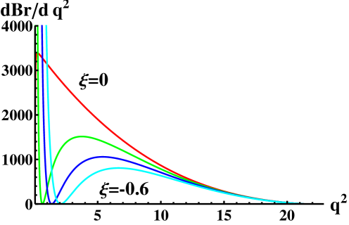
Figure 10: Behavior of $dBr/dq^{2}$ in the decay $B^{0}\rightarrow K^{0}\ell^{+}\ell^{-}$ in the unit of $G^{2}$ defined by Eq. (E.2). Curves are lined up in order of the cases $\xi=0$, $0.2$, $0.4$ and $0.6$ in the unit of GeV² (the colors red, green, blue and cyan, respectively).

References

[1] J.-T. Wei, et al. (Belle Collaboration),
Phys. Rev. Lett. 103 (2009) 171801.
[2]
J. P. Lees, et al. (BABAR Collaboration),
Phys. Rev. D 86 (2012) 032012.
[3]
R. Aaij et al. [LHCb Collaboration],
JHEP 1207 (2012) 133.
[4]
R. Aaij et al. [LHCb Collaboration],
JHEP 1302 (2013) 105.
[5]
T. Aaltonen et al. [CDF Collaboration],
Phys. Rev. Lett. 107 (2011) 201802.
[6]
A. Ali, P. Ball, L. T. Handoko and G. Hiller,
Phys. Rev. D 61 (2000) 074024 ;
A. Ali, E. Lunghi, C. Greub and G. Hiller,
Phys. Rev. D 66 (2002) 034002.
[7]
A. J. Buras,
hep-ph/9806471.
[8]
T. Feldmann and J. Matias,
JHEP 0301 (2003) 074.
[9]
C. Bobeth, G. Hiller, D. van Dyk and C. Wacker,
JHEP 1201 (2012) 107;
C. Hambrock, G. Hiller, S. Schacht and R. Zwicky,
arXive: 1308.4379 [hep-ph].
[10]
J. Lyon and R. Zwicky, arXive:1305.4797.
[11]
D. Becirevic, N. Kosnik, F. Mescia and E. Schneider,
Phys. Rev. D 86 (2012) 034034.
[12]
S. Jäger and J. M. Camalich,
JHEP 1305 (2013) 043.
[13]
M. Katuya and Y. Koide, Phys. Rev. D 19 (1979) 2631.
[14]
V. Luth, in Proceedings of the 1979 International
Symposium on Lepton and Photon Interaction at High Energy,
Fermilab, edited by T. B. W. Kirk and H. D. I. Abarbanel
(Fermilab, Batavia, Illinois, 1979); Report No.SLAC-PUB-2405,
LBL-9851.
[15]
M. Beneke, T. Feldmann and D. Seidel,
Nucl. Phys. B 612 (2001) 25.
[16]
A. Khodjamirian, Th. Mannel and Y.-M. Wang,
JHEP 1302 (2013) 010.
[17]
M. Beyer, D. Melikhov, N. Nikitin and B. Stech,
Phys. Rev. D 64 (2001) 094006;
S. W. Bosch and G. Buchalla,
Nucl. Phys. B 621 (2002) 459;
D. Melikhov and N. Nikitin, Phys. Rev. D 70 (2004) 114028.
[18]
Y. Koide and T. Yamashita,
Phys. Lett. B 711 (2012) 384.
[19]
S.L. Glashow, J. Iliopoulos, L. Maiani,
Phys. Rev. D 2 (1970) 1285.
[20]
Y. Koide, arXiv:1311.5320 [hep-ph].
[21]
Y. Sumino,
Phys. Lett. B 671 (2009) 477.
[22] Y. Koide, Phys. Rev. D 87 (2013), 016016.
[23]
Y. Koide,
Phys. Rev. D 23 (1981) 114.
[24]
B. Foster, A. D. Martin and M. G. Vincter, in Review of
Particle Physics, J. Beringer et al. (Particle Data Group),
Phys. Rev. D 86 (2012) 0100001.
[25]
Y. Y. Keum, M. Matsumori and A. I. Sanda,
Phys. Rev. D 72 (2005) 014013;
M. Matsumori and A. I. Sanda,
Phys. Rev. D 73 (2006) 114022.
[26]
H. Fusaoka and Y. Koide, Phys. Rev. D 57 (1998) 3986.
And see also, Z. -z. Xing, H. Zhang and S. Zhou,
Phys. Rev. D 77 (2008) 113016.
[27]
J. Beringer et al. (Particle Data Group),
Phys. Rev. D 86 (2012) 0100001.