Large eddy simulation of a muffler with the high-order spectral difference method

Abstract

The combination of the high-order accurate spectral difference discretization on unstructured grids with subgrid-scale modelling is investigated for large eddy simulation of a muffler at $Re=4.64\cdot 10^{4}$ and low Mach number. The subgrid-scale stress tensor is modelled by the wall-adapting local eddy-viscosity model with a cut-off length which is a decreasing function of the order of accuracy of the scheme. Numerical results indicate that although the high-order solver without subgrid-scale modelling is already able to capture well the features of the flow, the coupling with the wall-adapting local eddy-viscosity model improves the quality of the solution.

1 Introduction

Throughout the past two decades, the development of high-order accurate spatial discretization has been one of the major fields of research in computational fluid dynamics (CFD), computational aeroacoustics (CAA), computational electromagnetism (CEM) and in general computational physics characterized by linear and nonlinear wave propagation phenomena. High-order accurate discretizations have the potential to improve the computational efficiency required to achieve a desired error level. In fact, compared with low order schemes, high order methods offer better wave propagation properties and increased accuracy for a comparable number of degrees of freedom (DOFs). Therefore, it may be advantageous to use such schemes for problems that require very low numerical dissipation and small error levels [1]. Moreover, since computational science is increasingly used as an industrial design and analysis tool, high accuracy must be achieved on unstructured grids which are required for efficient meshing. These needs have been the driving force for the development of a variety of higher order schemes for unstructured meshes such as the Discontinuous Galerkin (DG) method [2, 3], the Spectral Volume (SV) method [4], the Spectral Difference (SD) method [5, 6], the Energy Stable Flux Reconstruction [7] and many others.

In this study we focus on a SD solver for unstructured hexahedral grids (tensorial cells). The SD method has been proposed as an alternative high order collocation-based method using local interpolation of the strong form of the equations. Therefore, the SD scheme has an important advantage over classical DG and SV methods, that no integrals have to be evaluated to compute the residuals, thus avoiding the need for costly high-order accurate quadrature formulas.

Although the formulation of high-order accurate spatial discretization is now fairly mature, their application for the simulation of general turbulent flows implies that particular attention has still to be paid to subgrid-scale (SGS) models. So far, the combination of the SD method with SGS models for LES has not been widely investigated. In 2010, Parsani et al. [8] reported the first implementation in study of a two-dimensional (2D) third-order accurate SD solver coupled with the Wall-Adapting Local Eddy-viscosity (WALE) model [14] and a cut-off length which is a decreasing function of the order of accuracy. A successful extension of that approach to a three-dimensional (3D) second-order accurate SD solver has been reported in [12]. Very recently, Lodato and Jameson [13] have presented an alternative technique to model the unresolved scales in the flow field: A structural SGS approach with the WALE Similarity Mixed model (WSM), where constrained explicit filtering represents a key element to approximate subgrid-scale interactions. The performance of such an algorithm has been also satisfactory.

In this study, we couple for the first time the approach proposed in [8] with a 3D fourth-order accurate SD solver, for the simulation of the turbulent flow in an industrial-type muffler at $Re=4.64\cdot 10^{4}$. The goal is to investigate if the coupling of a high-order SD scheme with a sub-grid closure model improves the quality of the results when the grid resolution is relatively low. The latter requirement is often desirable when a high-order accurate spatial discretization is used.

2 Physical model and numerical algorithm

In this study the system of the Navier-Stokes equations for a compressible flow are discretized in space using the SD method and the subgrid-scale stress tensor is modelled by the WALE approach.

2.1 Filtered Navier-Stokes equations

The three physical conservation laws for a general Newtonian fluid, i.e., the continuity, the momentum and energy equations, are introduced using the following notation: $\rho$ for the mass density, $\vec{u}\in\mathbb{R}^{dim}$ for the velocity vector in a physical space with $dim$ dimensions, $P$ for the static pressure and $E$ for the specific total energy which is related to the pressure and the velocity vector field by $E=\frac{1}{\gamma-1}\frac{P}{\rho}+\frac{|\vec{u}|^{2}}{2}$, where $\gamma$ is the constant ratio of specific heats and it is $1.4$ for air in standard conditions.

The system, written in divergence form and equipped with suitable initial-boundary conditions, is

$$\frac{\partial\textbf{w}}{\partial t}+\vec{\nabla}\cdot\left(\vec{\textbf{f}}_{C}\left(\textbf{w}\right)-\vec{\textbf{f}}_{D}\left(\textbf{w},\vec{\nabla}\textbf{w}\right)\right)=\frac{\partial\textbf{w}}{\partial t}+\vec{\nabla}\cdot\vec{\textbf{f}}=0,$$ (1)

where $\textbf{w}=\left(\overline{\rho},\overline{\rho}\tilde{\vec{u}},\overline{\rho}\tilde{E}\right)^{T}$ is the vector of the filtered conservative variables and $\vec{\textbf{f}}_{C}=\vec{\textbf{f}}_{C}\left(\textbf{w}\right)$ and $\vec{\textbf{f}}_{D}=\vec{\textbf{f}}_{D}\left(\textbf{w},\vec{\nabla}\textbf{w}\right)$ represent the convective and the diffusive fluxes, respectively. Here the symbols $(\overline{\cdot})$ and $(\tilde{\cdot})$ represent the spatially filtered field and the Favre filtered field defined as $\tilde{\vec{u}}=\overline{\rho\vec{u}}/\overline{\rho}$.

In a general 3D ($dim=3$) Cartesian space, $\vec{x}=\left[x_{1},x_{2},x_{3}\right]^{T}$, the components of the flux vector $\vec{\textbf{f}}\left(\textbf{w},\vec{\nabla}\textbf{w}\right)=\left[\textbf{f}_{1},\textbf{f}_{2},\textbf{f}_{3}\right]^{T}$ are given by

$$\textbf{f}_{1}=\left(\begin{array}[]{c}\overline{\rho}\tilde{u}_{1}\\ \overline{\rho}\tilde{u}_{1}^{2}+\overline{P}-\tilde{\sigma}_{11}+\tau_{11}^{sgs}\\ \overline{\rho}\tilde{u}_{1}\tilde{u}_{2}-\tilde{\sigma}_{21}+\tau_{21}^{sgs}\\ \overline{\rho}\tilde{u}_{1}\tilde{u}_{3}-\tilde{\sigma}_{31}+\tau_{31}^{sgs}\\ \tilde{u}_{1}\left(\overline{\rho}\tilde{E}+\overline{P}\right)-\tilde{u}_{1}\left(\tilde{\sigma}_{11}-\tau_{11}^{sgs}\right)-\tilde{u}_{2}\left(\tilde{\sigma}_{21}-\tau_{21}^{sgs}\right)-\tilde{u}_{3}\left(\tilde{\sigma}_{31}-\tau_{31}^{sgs}\right)-c_{P}\frac{\mu}{Pr}\frac{\partial\tilde{T}}{\partial x_{1}}+q_{1}^{sgs}\end{array}\right),$$

$$\textbf{f}_{2}=\left(\begin{array}[]{c}\overline{\rho}\tilde{u}_{2}\\ \overline{\rho}\tilde{u}_{1}\tilde{u}_{2}-\tilde{\sigma}_{12}+\tau_{12}^{sgs}\\ \overline{\rho}\tilde{u}_{2}^{2}+\overline{P}-\tilde{\sigma}_{22}+\tau_{22}^{sgs}\\ \overline{\rho}\tilde{u}_{2}\tilde{u}_{3}-\tilde{\sigma}_{32}+\tau_{32}^{sgs}\\ \tilde{u}_{2}\left(\overline{\rho}\tilde{E}+\overline{P}\right)-\tilde{u}_{1}\left(\tilde{\sigma}_{12}-\tau_{12}^{sgs}\right)-\tilde{u}_{2}\left(\tilde{\sigma}_{22}-\tau_{22}^{sgs}\right)-\tilde{u}_{3}\left(\tilde{\sigma}_{32}-\tau_{32}^{sgs}\right)-c_{P}\frac{\mu}{Pr}\frac{\partial\tilde{T}}{\partial x_{2}}+q_{2}^{sgs}\end{array}\right),$$

$$\textbf{f}_{3}=\left(\begin{array}[]{c}\overline{\rho}\tilde{u}_{3}\\ \overline{\rho}\tilde{u}_{1}\tilde{u}_{3}-\tilde{\sigma}_{13}+\tau_{13}^{sgs}\\ \overline{\rho}\tilde{u}_{2}\tilde{u}_{3}-\tilde{\sigma}_{23}+\tau_{23}^{sgs}\\ \overline{\rho}\tilde{u}_{3}^{2}+\overline{P}-\tilde{\sigma}_{33}+\tau_{33}^{sgs}\\ \tilde{u}_{3}\left(\overline{\rho}\tilde{E}+\overline{P}\right)-\tilde{u}_{1}\left(\tilde{\sigma}_{13}-\tau_{13}^{sgs}\right)-\tilde{u}_{2}\left(\tilde{\sigma}_{23}-\tau_{23}^{sgs}\right)-\tilde{u}_{3}\left(\tilde{\sigma}_{33}-\tau_{33}^{sgs}\right)-c_{P}\frac{\mu}{Pr}\frac{\partial\tilde{T}}{\partial x_{3}}+q_{3}^{sgs}\end{array}\right),$$

where $c_{P}$, $\mu$, $Pr$ and $T$ represent respectively the specific heat capacity at constant pressure, the dynamic viscosity, the Prandtl number and the temperature of the fluid. Moreover, $\sigma_{ij}$ represents the $ij-$component of the resolved viscous stress tensor [15].

Both momentum and energy equations differ from the classical fluid dynamic equations only for two terms which take into account the contributions from the unresolved scales. These contributions, represented by the specific subgrid-scale stress tensor $\tau_{ij}^{sgs}$ and by the subgrid heat flux vector defined $q_{i}^{sgs}$, appear when the spatial filter is applied to the convective terms [15]. The interactions of $\tau_{ij}^{sgs}$ and $q_{i}^{sgs}$ with the resolved scales have to be modeled through a subgrid-scale closure model because they cannot be determined using only the resolved flow field w.

2.1.1 The wall-adapted local eddy-viscosity closure model

The smallest scales present in the flow field and their interaction with the resolved scales have to be modeled through the subgrid-scale term $\tau_{ij}^{sgs}$. The most common approach to model such a tensor is based on the eddy-viscosity concept in which one assumes that the residual stress is proportional to a measure of the filtered local strain rate [15], which is defined as follows:

$$\tau_{ij}^{sgs}-\tau_{kk}^{sgs}\delta_{ij}=-2\,\overline{\rho}\,\nu_{t}\left(\tilde{S}_{ij}-\frac{\delta_{ij}}{3}\tilde{S}_{kk}\right).$$ (2)

In the WALE model, it is assumed that the eddy-viscosity $\nu_{t}$ is proportional to the square of the length scale of the cut-off length (or width of the grid filter) and the filtered local rate of strain. Although the model was originally developed for incompressible flows, it can also be used for variable density flows by giving the formulation as follows

$$\nu_{t}=\left(C\Delta\right)^{2}\left|\tilde{S}\right|.$$ (3)

Here $\left|\tilde{S}\right|$ is defined as

$$\left|\tilde{S}\right|=\frac{\left[\tilde{S}_{ij}^{d}\,\tilde{S}_{ij}^{d}\right]^{3/2}}{\left[\tilde{S}_{ij}\,\tilde{S}_{ij}\right]^{5/2}+\left[\tilde{S}_{ij}^{d}\,\tilde{S}_{ij}^{d}\right]^{5/4}},$$ (4)

where $\tilde{S}_{ij}^{d}$ is the traceless symmetric part of the square of the resolved velocity gradient tensor $\tilde{g}_{ij}=\frac{\partial\tilde{u}_{i}}{\partial x_{j}}$. Note that in Equation (3) $\Delta$, i.e., the cut-off length, is an unknown function. Often the cut-off length is taken proportional to the smallest resolvable length scale of the discretization. In the present work, the definition of the grid filter function is given in Section 2.2, where the SD method is discussed.

2.2 Spectral difference method

Consider a problem governed by a general system of conservation laws given by Equation (1) and valid on a domain $\Omega\subset\mathbb{R}^{dim}$ with boundary $\partial\Omega$ and completed with consistent initial and boundary conditions. The domain is divided into $N$ non-overlapping cells, with cell index $i$.

In order to achieve an efficient implementation of the SD method, all hexahedral cells in the physical domain are mapped into cubic elements using local coordinates $\vec{\xi}=\left[\xi_{1},\xi_{2},\xi_{3}\right]^{T}$. Such a transformation is characterized by the Jacobian matrix $\vec{\vec{\left.\mathrm{J}\right.}}_{i}$ with determinant $det(\vec{\vec{\left.\mathrm{J}\right.}}_{i})$. Therefore, system (1) can be written in the mapped coordinate system as

$$\frac{\partial\mathbf{w}_{i}^{\hskip 1.13791pt\vec{\xi}}}{\partial t}=-\frac{\partial\mathbf{f}_{1,i}^{\hskip 1.13791pt\vec{\xi}}}{\partial\xi_{1}}-\frac{\partial\mathbf{f}_{2,i}^{\hskip 1.13791pt\vec{\xi}}}{\partial\xi_{2}}-\frac{\partial\mathbf{f}_{3,i}^{\hskip 1.13791pt\vec{\xi}}}{\partial\xi_{3}}=-\vec{\nabla}^{\hskip 1.13791pt\vec{\xi}}\cdot\vec{\textbf{f}}^{\hskip 1.13791pt\vec{\xi}}_{i},$$ (5)

where $\mathbf{w}^{\hskip 1.13791pt\vec{\xi}}_{i}\equiv det(\vec{\vec{\left.\mathrm{J}\right.}}_{i})\,\mathbf{w}$ and $\vec{\nabla}^{\hskip 1.13791pt\vec{\xi}}$ are the conserved variables and the generalized divergence differential operator in the mapped coordinate system, respectively.

For a $\left(p+1\right)$-th-order accurate $dim$-dimensional scheme, $N^{s}$ solution collocation points with index $j$ are introduced at positions $\vec{\xi}_{j}^{s}$ in each cell $i$, with $N^{s}$ given by $N^{s}=\left(p+1\right)^{dim}$. Given the values at these points, a polynomial approximation of degree $p$ of the solution in cell $i$ can be constructed. This polynomial is called the solution polynomial and is usually composed of a set of Lagrangian basis polynomial $L_{j}^{s}\left(\vec{\xi}\right)$ of degree $p$:

$$\mathbf{W}_{i}\left(\vec{\xi}\right)=\sum_{j=1}^{N^{s}}\mathbf{W}_{i,j}\,L_{j}^{s}\left(\vec{\xi}\right).$$ (6)

Therefore, the unknowns of the SD method are the interpolation coefficients $\mathbf{W}_{i,j}=\mathbf{W}_{i}\left(\vec{\xi}_{j}^{s}\right)$ which are the approximated values of the conserved variables $\mathbf{w}_{i}$ at the solution points.

The divergence of the mapped fluxes $\vec{\nabla}^{\hskip 1.13791pt\vec{\xi}}\cdot\vec{\textbf{f}}^{\hskip 1.13791pt\vec{\xi}}$ at the solution points is computed by introducing a set of $N^{f}$ flux collocation points with index $l$ and at positions $\vec{\xi}_{l}^{f}$, supporting a polynomial of degree $p+1$. The evolution of the mapped flux vector $\vec{\textbf{f}}^{\hskip 1.13791pt\vec{\xi}}$ in cell $i$ is then approximated by a flux polynomial $\vec{\textbf{F}}^{\hskip 1.13791pt\vec{\xi}}_{i}$, which is obtained by reconstructing the solution variables at the flux points and evaluating the fluxes $\vec{\textbf{F}}^{\hskip 1.13791pt\vec{\xi}}_{i,l}$ at these points. The flux is also represented by a Lagrange polynomial:

$$\vec{\textbf{F}}^{\hskip 1.13791pt\vec{\xi}}_{i}\left(\vec{\xi}\right)=\sum_{l=1}^{N^{f}}\vec{\textbf{F}}^{\hskip 1.13791pt\vec{\xi}}_{i,l}\,L_{l}^{f}\left(\vec{\xi}\right),$$ (7)

where the coefficients of the flux interpolation are defined as

$$\vec{\textbf{F}}^{\hskip 1.13791pt\vec{\xi}}_{i,l}=\begin{cases}\vec{\textbf{F}}^{\hskip 1.13791pt\vec{\xi}}_{i}\left(\vec{\xi}_{l}^{f}\right),&\quad\vec{\xi}_{l}^{f}\in\Omega_{i},\\ \vec{\textbf{F}}_{\mathrm{num}}^{\hskip 1.13791pt\vec{\xi}}\left(\vec{\xi}_{l}^{f}\right),&\quad\vec{\xi}_{l}^{f}\in\partial\Omega_{i}.\end{cases}$$ (8)

Here $\vec{\textbf{F}}_{\mathrm{num}}^{\hskip 1.13791pt\vec{\xi}}$ is the numerical flux vector at the cell interface. In fact, the solution at a face is in general not continuous and requires the solution of a Riemann problem to maintain conservation at a cell level (i.e., the flux component normal to a face $\vec{\textbf{F}}_{\mathrm{num}}^{\hskip 1.13791pt\vec{\xi}}\cdot\vec{n}^{\hskip 1.13791pt\vec{\xi}}$ must be continuous between two neighboring cells). Approximate Riemann solvers are typically used (e.g. Rusanov Riemann solver). The tangential component of $\vec{\textbf{F}}_{\mathrm{num}}^{\hskip 1.13791pt\vec{\xi}}$ is usually taken from the interior cell.

Taking the divergence of the flux polynomial $\vec{\nabla}^{\hskip 1.13791pt\vec{\xi}}\cdot\vec{\textbf{F}}^{\hskip 1.13791pt\vec{\xi}}_{i}$ in the solution points results in the following modified form of (5), describing the evolution of the conservative variables at the solution points:

$$\frac{d\mathbf{W}_{i,j}}{dt}=-\left.\vec{\nabla}\cdot\vec{\textbf{F}}_{i}\right|_{j}=-\frac{1}{J_{i,j}}\left.\vec{\nabla}^{\hskip 1.13791pt\vec{\xi}}\cdot\vec{\textbf{F}}^{\hskip 1.13791pt\vec{\xi}}_{i}\right|_{j}=\mathbf{R}_{i,j},$$ (9)

where $\vec{\textbf{F}}_{i}$ is the flux polynomial vector in the physical space whereas $\mathbf{R}_{i,j}$ is the SD residual associated with $\mathbf{W}_{i,j}$. This is a system of ODEs, in time, for the unknowns $\mathbf{W}_{i,j}$. In this work, the optimized explicit eighteen-stages fourth-order Runge-Kutta schemes presented in [16] is used to solve such a system at each time step.

2.2.1 Solution and flux points distributions

In 2007, Huynh [9] showed that for quadrilateral and hexahedral cells, tensor product flux point distributions based on a one-dimensional flux point distribution consisting of the end points and the Legendre-Gauss quadrature points lead to stable schemes for arbitrary order of accuracy. In 2008, Van den Abeele et al. [10] showed an interesting property of the SD method, namely that it is independent of the positions of its solution points in most general circumstances. This property implies an important improvement in efficiency, since the solution points can be placed at flux point positions and thus a significant number of solution reconstructions can be avoided. Recently, this property has been proved by Jameson [11].

2.2.2 Cut-off length $\Delta$

In Section 2.1.1 we have seen that in the WALE model the cut-off length $\Delta$ is used to compute the turbulent eddy-viscosity $\nu_{t}$, i.e., Equation (3). Following the approach presented in [8], for each cell with index $i$ and each flux points with index $l$ and positions $\boldsymbol{\xi}_{l}^{f}$, we use the following definition of filter width

$$\Delta_{i,l}=\left[\frac{1}{N^{s}}det\left(\left.\vec{\vec{\left.\mathrm{J}\right.}}_{i}\right|_{\boldsymbol{\xi}_{l}^{f}}\right)\right]^{1/dim}=\left(\frac{det(J_{i,l})}{N^{s}}\right)^{1/dim}.$$ (10)

Notice that the cell filter width is not constant in one cell, but it varies because the Jacobian matrix is a function of the positions of the flux points. Moreover, for a given mesh, the number of solution points depends on the order of the SD scheme, so that the grid filter width decreases by increasing the polynomial order of the approximation.

3 Numerical results

The main purpose of this section is to evaluate the accuracy and the reliability of the fourth-order SD-LES solver for simulating a 3D turbulent flow in an industrial-type muffler. The results are compared with the particle image velocimetry (PIV) measurement performed at the Department of Environmental and Applied Fluid Dynamics of the von Karman Institute for Fluid Dynamics [17]. In Figure 1, the geometry of the muffler and its characteristic dimensions are illustrated, where the flow is from left to right.

Figure 1: Configuration of the 3D muffler test case.

At the inlet, mass density and velocity profiles are imposed. The inlet velocity profile in the $x_{3}$ direction is given by

$$u_{3}=u_{max}\left\{\frac{1}{2}-\frac{1}{2}\tanh{\left[2.2\left(\frac{r}{d/2}-\frac{d/2}{r}\right)\right]}\right\}.$$

At the outlet only the pressure is prescribed. In accordance to the experiments, the inlet Mach number and the Reynolds number, based on maximum velocity at the inlet $u_{max}$ and the diameter of the inlet/outlet $d$ ($d=4\,cm$), are set respectively to $M_{inlet}=0.05$ and $Re=4.64\cdot 10^{4}$.

The flow is computed using fourth-order ($p=3$) SD scheme on a grid with $36,612$ hexahedral elements which was generated with the open source software Gmsh [18]. Second-order boundary elements are used to approximate the curved geometry. The total number of DOFs is approximately $2.3\cdot 10^{6}$ (i.e., $36,612\cdot(p+1)^{3}$). The maximum CFL number used for the computations started from $0.1$ and increased up to $0.65$. After the flow field was fully developed, time averaging is performed for a period corresponding to about 25 flow-through times.

The computation is validated on the center plane of the expansion coinciding with the center planes of the inlet and outlet pipes using the PIV results from [17]. All of the measurements are taken on the symmetrical center plane of the muffler. The reference cross section corresponds to the entrance of the expansion chamber. It should be noted that the circular nature of the geometry acts as a lens causing a change in magnification in the radial direction ($x_{2}$) which prevents from capturing images close to the wall. It is found that outside $~{}1\,cm$ from the wall the magnification effect is negligible and as the mean stream-wise direction is in the direction of constant magnification and has only little effect on the particle correlations no corrections are deemed necessary.

In Figure 2, the non-dimensional mean velocity profile in the axial direction $\langle\tilde{u}_{3}\rangle/u_{max}$ is shown for four different cross sections in the expansion chamber, where the PIV measurements were done. In this figure, the PIV data are also plotted for comparison. Figure 3 shows the non-dimensional Reynolds stress $\langle u_{2}^{\prime}u_{3}^{\prime}\rangle/{u_{max}^{2}}$ at the same cross sections. Although the high-order implicit LES is already able to capture well the features of the flow field, the use of the WALE model improves the results. In particular, when the SGS model is active, the local extrema of the time-averaged velocity profiles and the second-order statistical moment (which get fairly oscillatory by moving far away from the inlet pipe) are better captured.

4 Conclusions

The fourth-order SD method in combination with the WALE model and the variable filter width performed well. The numerical results confirm that the model is correctly accounting for the unresolved shear stress computed from the resolved field, for the present internal flow. However, it should be noted that the SD discretization without subgrid-scale modelling also worked rather well, at least for the grid resolution used in this study.

Work is currently under way to test both approaches for different orders of accuracy, grid resolutions and other realistic turbulent flows. We believe that the flexibility of the high-order SD scheme on unstructured grids together with the development of robust sub-grid closure models for highly separated flows and efficient grid generators for high-order accurate schemes will allow to perform LES of industrial-type flows in the near future.

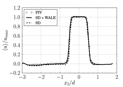
(a) $1d$ downstream.

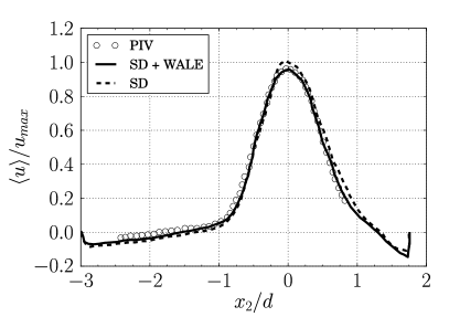
(b) $4d$ downstream.

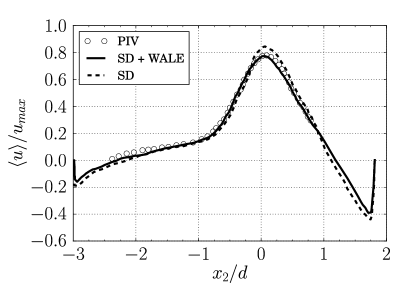
(c) $6d$ downstream.

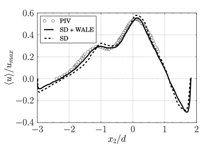
(d) $7d$ downstream.

Figure 2: Time-averaged velocity profile in the axial direction $\langle\tilde{u}_{3}\rangle/u_{max}$ at four cross sections in the expansion chamber, obtained with fourth-order ($p=3$) SD-LES method. Comparison with experimental measurements (PIV) [17].

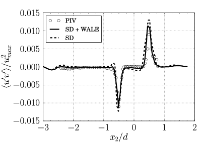
(a) $1d$ downstream.

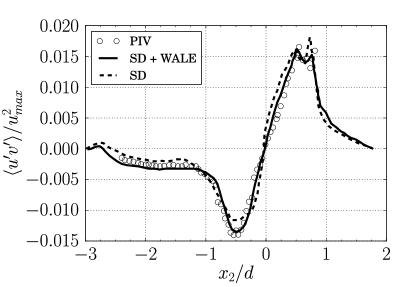
(b) $4d$ downstream.

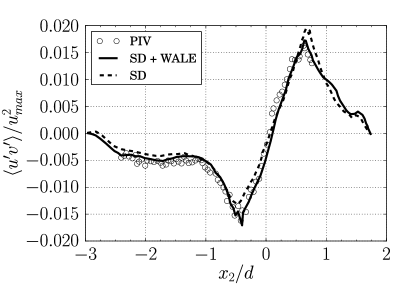
(c) $6d$ downstream.

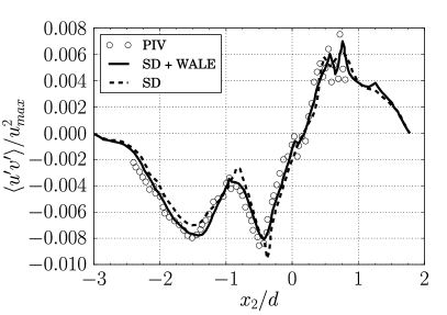
(d) $7d$ downstream.

Figure 3: Reynolds stress $\langle u_{2}^{\prime}u_{3}^{\prime}\rangle/u_{max}^{2}$ in the axial direction at four cross sections in the expansion chamber, obtained with fourth-order ($p=3$) SD-LES method. Comparison with experimental measurements (PIV) [17].

References

- [1] Wang, Z. J.: Adaptive High-order Methods in Computational Fluid Dynamics (Advances in Computational Fluid Dynamics), World Scientific Publishing Company (2011).
- [2] Busch, K., König, M., and Niegemann, J.: Discontinuous Galerkin methods in nanophotonics. Laser Photonics Rev. 5(6), 773–809 (2011).
- [3] Hesthaven, Jan S., and Warburton, Tim: Nodal Discontinuous Galerkin Methods: Algorithms, Analysis, and Applications. Texts in Applied Mathematics, 54. Computational Science & Engineering, Springer Publishing Company, Incorporated (2007).
- [4] Sun, Y., Wang, Z. J., and Liu Y.: Spectral (finite) volume method for conservation laws on unstructured grids VI: extension to viscous flow. J. of Comput. Phys., 215(1), 41–58 (2006).
- [5] May, G., and Jameson, A.: A spectral difference method for the Euler and Navier-Stokes equations on unstructured meshes. AIAA paper 2006-304. 44th AIAA Aerospace Sciences Meeting, Reno, Nevada, USA, January 9-12, 2006.
- [6] Sun, Y., Wang, Z. J., and Liu, Y.: High-order multidomain spectral difference method for the Navier-Stokes equations on unstructured hexahedral grids. Commun. Comput. Phys, 2(2), 310–333 (2007).
- [7] Castonguay, P., Vincent P., and Jameson, A.: Application of High-Order Energy Stable Flux Reconstruction Schemes to the Euler Equations. AIAA paper 2011-686. 49th AIAA Aerospace Sciences Meeting including the New Horizons Forum and Aerospace Exposition, Orlando, Florida, USA, January 4-7, 2011.
- [8] Parsani, M., Ghorbaniasl, G., Lacor C., and Turkel, E.: An implicit high-order spectral difference approach for large eddy simulation. J. Comput. Phys., 229(14), 5373–5393 (2010).
- [9] Huynh, H. T.: A flux reconstruction approach to high-order schemes including discontinuous Galerkin methods. AIAA paper 2007-4079. 18th AIAA Computational Fluid Dynamics Conference, Miami, Florida, USA, June 25-28, 2007.
- [10] Van den Abeele, K., Lacor, C., and Wang, Z. J.: On the stability and accuracy of the spectral difference method, J. Sci. Comput., 37(2), 162–188 (2008).
- [11] Jameson, A.: A proof of the stability of the spectral difference method for all orders of accuracy, J. Sci. Comput., 45(1-3), 348–358 (2010).
- [12] Parsani, M., Ghorbaniasl, G., and Lacor C.: Validation and application of an high-order spectral difference method for flow induced noise simulation. J. Comput. Acoust., 19(3), 241–268 (2011).
- [13] Lodato, G., and Jameson, A.: LES modeling with high-order flux reconstruction and spectral difference schemes. ICCFD paper 2201. 7th ICCFD Conference, Big Island, Hawaii, July 9-13, 2012.
- [14] Nicoud, F., and Ducros, F.: Subgrid-scale stress modelling based on the square of the velocity gradient tensor. Flow Turbul. Combust., 62(3), 183–200 (1999).
- [15] Pope, Stephen B.: Turbulent flows. Cambridge University Press (2003).
- [16] Parsani, M., Ketcheson, David I., and Deconinck, W.: Optimized explicit Runge-Kutta schemes for the spectral difference method applied to wave propagation problems, SIAM J. Sci. Comput, 35(2):A957-A986 (2013).
- [17] Bilka, M., and Anthoine, J.: Experimental investigation of flow noise in a circular expansion using PIV and acoustic measurements. AIAA paper 2008-2952. 14th AIAA/CEAS Aeroacoustics Conference, Vancouver, British Columbia, Canada, May 5-6, 2008.
- [18] Geuzaine, C., and Remacle J.-F.: Gmsh: a three-dimensional finite element mesh generator with built-in pre- and post-processing facilities. Int. J. Numer. Meth. Eng., 79(11), 1309–1331 (2009).