Abstract

Causal Dynamical Triangulations provide a non-perturbative regularization of a theory of quantum gravity. We describe how this approach connects with the asymptotic safety program and Hořava-Lifshitz gravity theory, and present the most recent results from computer simulations.

keywords: MG13 Proceedings. Plenary talk. Quantum gravity.

1 Introduction

We do not know if there exists a theory of quantum gravity and precisely how we should think about quantizing geometry. The amazing successes of quantum mechanics and quantum field theory have been obtained in the rigid background of flat spacetime. Can we extend the realm of quantization to include the geometry of spacetime itself in a consistent way? Even if the answer is affirmative (as will be argued shortly), we are still faced with the problem that starting out with general relativity (GR) and expanding around a fixed classical background geometry, the gravitational fluctuations are non-renormalizable in a conventional field-theoretical sense.

How should we deal with the non-renormalizable aspects? The logic behind string theory is in a sense in line with how non-renormalizable theories have been handled until now. Two examples in point are the four-fermion model of the weak interactions and the non-linear sigma model of pion interactions. In both cases new degrees of freedom were introduced, which made the more fundamental, underlying field theories renormalizable. The apparent non-renormalizability of the models was due to our incomplete understanding of the underlying short-distance physics. String theory introduces an infinite number of new field degrees of freedom in order to tame the UV divergences of the gravitational field. This solution to the UV problem has a certain elegance, since it can be described as moving from zero-dimensional point particles to one-dimensional strings in an (almost) unique way, dictated by relativistic invariance. When the string is expanded into modes, one is led to an infinite set of fields. However, despite the presence of an enormous number of degrees of freedom string theory has had difficulties reproducing anything like the universe we observe. Loop quantum gravity and its ramifications constitute other attempts to define a theory of quantum gravity [1]. In loop quantum gravity one insists that holonomies are quantum objects which are finite. This leads to a somewhat non-standard quantization with non-separable Hilbert spaces, and it is in general difficult to show that one obtains a $\hbar\to 0$ limit which can be identified with classical GR.

The asymptotic safety program [2] tries to address the problem of non-renormalizability in a more mundane way, using only ordinary quantum field theory. It appeals to the Wilsonian concept of renormalizability, where the UV or IR behaviour of a quantum field theory are linked to the existence of fixed points of the renormalization group. Accordingly, in this framework one conjectures that the behaviour of quantum gravity at high energies is governed by a non-Gaussian fixed point in the UV, which has properties similar to the Gaussian UV fixed point known from renormalizable quantum field theories. In a renormalizable theory with a Gaussian UV fixed point, sufficiently close to it there are only a finite number of independent operators that take us away from the fixed point when we integrate out high-frequency modes. Furthermore, the coupling constants associated with these operators scale to zero at the fixed point. For a Gaussian UV fixed point in flat spacetime we can (except for possible complications with gauge invariance etc.) obtain the possible operators by power counting. The associated coupling constants are in principle the only ones that need fine-tuning in order to reach the fixed point. One can use perturbation theory to check this picture when one is close to the Gaussian fixed point. Asymptotic safety assumes that a similar scenario is valid for a putative non-Gaussian fixed point, the only problem being that we currently have no examples of such non-Gaussian UV fixed points in four-dimensional conventional quantum field theory. Since the fixed point in question is non-Gaussian, we do not have perturbation theory available to investigate it. It is nevertheless a logical possibility that such a fixed point exists precisely in the case of quantum gravity. Over the last 20 years investigations using improved renormalization group techniques[3], as well as 2+$\varepsilon$ dimension expansions[4] have produced some evidence for the existence of such a UV fixed point for quantum gravity.

Finally, a simple way to address the non-renormalizability issue using only conventional quantum field theory has more recently been suggested by Hořava and since been dubbed Hořava-Lifshitz gravity[5]. It emphasizes unitarity and the requirement that the theory should be renormalizable. It achieves this by insisting on at most second-order time derivatives in the action but allowing for higher-order spatial derivatives. The price one pays is that the theory violates Lorentz invariance at short distances where the higher-derivative terms are important, the hope being that – in agreement with observations – the Lorentz invariance is approximately restored at large distances.

Causal dynamical triangulations (CDT) is a lattice regularization of quantum gravity[6, 7]. It provides us with a non-perturbative definition of the path integral of quantum gravity, where the length of the lattice links $a$ acts as a UV cut-off. Formally, the continuum limit is obtained when $a\to 0$. As a lattice theory it fits naturally into a Wilsonian framework and can therefore be thought of as an independent way of investigating the asymptotic safety scenario; one has a phase diagram in terms of the bare coupling constants and looks for second-order phase transition points which can serve as the non-Gaussian UV fixed points of asymptotic safety. Having identified such fixed points one can study the renormalization group flow close to them. At the same time, CDT is well suited to serve as a regularization of Hořava-Lifshitz (HL) gravity models, since both in CDT and HL gravity one integrates in the path integral over geometries which have a preferred time foliation. As will be discussed below, the CDT phase diagram also has many similarities with a Lifshitz phase diagram.

Before entering the detailed discussion of CDT results, let us discuss three key issues:

• Does it make sense to talk about a quantum theory of gravity, which includes fluctuating geometries, when conventional quantization is always performed with reference to a fixed geometry?

• Does it make sense to consider a lattice regularization of a diffeomorphism-invariant theory?

• Does it make sense to talk about a Wilsonian framework in a diffeomorphism-invariant theory, where one has not even defined what is meant by a (diffeomorphism-invariant) correlation length?

As it happens, all of the above questions can be answered affirmatively without addressing the more difficult question of whether there exists a quantum gravity theory in four-dimensional spacetime. In two dimensions, gravity becomes a very simple theory, since the integral of the scalar curvature is topological. Thus there is no dynamical action. Nevertheless the theory has a non-trivial partition function, and produces non-trivial amplitudes for universes with one boundary geometry “propagating” into another boundary geometry and for matter fields living on such fluctuating geometries. Of course, this theory has no propagating local gravitational degrees of freedom. However, the conceptual questions mentioned above do not really refer to the propagation of gravitational degrees of freedom, but to the fact that we are dealing with fluctuating geometry, in a setting where we only want to ask diffeomorphism-invariant questions. Viewed in this perspective, one could even say that the two-dimensional theory provides us with the ultimate test, since there hardly is any classical action (only the cosmological term). If we think about the quantum theory using the path integral as a sum over spacetime histories, we are dealing with a situation that is “maximally quantum”, in the sense that each configuration in the path integral has the same weight. This corresponds formally to the limit $\hbar\to\infty$, i.e. the ultimate quantum limit.

So-called 2d Liouville quantum gravity can be solved analytically, both using canonical quantization and the path integral. It is the quantum theory of fluctuating two-dimensional geometries with fixed topology, and therefore answers (1) above. The same theory can be regularized using lattices, using the formalism called “dynamical triangulations” (DT). In it one performs the path integral in the Euclidean sector by using equilateral triangles as building blocks, and gluing them together in all possible ways compatible with the given topology. In this way the path integral becomes the sum over a class of piecewise linear geometries, whose geometry is determined entirely by the way the building blocks are glued together, justifying the name “dynamical triangulations”. The link length $a$ of the building blocks acts as a UV cut-off. Somewhat surprisingly, one can solve this lattice theory analytically and in the limit $a\to 0$ recover the continuum quantum Liouville results. In other words, there exists a lattice regularization where one sums over spacetime geometries (as opposed to spacetime metrics), no gauge-fixing is needed (and therefore no issue of diffeomorphism-invariance arises), and the $a\to 0$ limit leads to a diffeomorphism-invariant theory, namely, quantum Liouville theory.

The lattice theory also fits beautifully into a Wilsonian framework, thereby answering question (3) above. To start with, it has universality in the sense that we are not restricted to using equilateral triangles as building blocks. Using instead almost any ensemble of polygons with side-length $a$, and gluing them together with almost any positive weights, the continuum limit $a\to 0$ will still be the same. By adding suitable higher-curvature action terms to this theory of planar graphs one again obtains the same continuum limit, demonstrating a Wilsonian universality with respect to both regularization and the choice of action.

Finally, is it possible to define the concept of diffeomorphism-invariant correlators depending on a diffeomorphism-invariant correlation length? In two dimensions, where we have no propagating gravitational field degrees of freedom, one has to add matter fields to the fluctuating geometries to answer this question. This can be done, and the answer is again in the affirmative [8]. To be more explicit, let us consider a matter field $\phi(x)$, whose dynamics is governed by some diffeomorphism-invariant action. Clearly it makes no sense to consider the correlation between two local fields $\phi(x)$ and $\phi(y)$, since $x$ and $y$ are just coordinates. In addition, since the geometry of spacetime is fluctuating, the geodesic distance between $x$ and $y$ will depend on the geometry, and we are summing over these geometries. How do we then define a meaningful diffeomorphism-invariant correlation between fields? In flat $d$-dimensional spacetime, let us rewrite the correlator of the scalar field $\phi(x)$ in the form

$$\langle\phi\phi(R)\rangle_{V}\equiv\frac{1}{V}\;\frac{1}{s(R)}\int{\cal D}\phi\,e^{-S[\phi]}\int\!\!d^{d}x\!\int\!\!d^{d}y\;\phi(x)\phi(y)\;\delta(R\!-\!|x-y|).$$ (1)

As indicated, this expression depends on a chosen distance $R$, but no longer on specific points $x$ and $y$, which instead are integrated over. The integrand can be read “from right to left” as first averaging over all points $y$ at a distance $R$ from some fixed point $x$, normalized by the volume $s(R)$ of the spherical shell of radius $R$, and then averaging over all points $x$, normalized by the total volume $V$ of spacetime. We assume translational and rotational invariance of the theory and that $V$ is so large that we can ignore any boundary effects related to a finite volume. This definition of a correlator is of course non-local, but unlike the underlying locally defined correlator has a straightforward diffeomorphism-invariant generalization to the case where gravity is dynamical, namely,

$$\langle\phi\phi(R)\rangle_{V} \equiv \frac{1}{V}\int{\cal D}[g]\,\int{\cal D}_{[g]}\phi\;\mbox{e}^{-S[g,\phi]}\;\delta\Big{(}V-\!\!\int\!\!d^{d}x\sqrt{\det g}\Big{)}\times$$ (2)

$$\int\!\!d^{d}x\!\int\!\!d^{d}y\,\;\frac{\sqrt{\det g(x)}\,\sqrt{\det g(y)}}{s_{[g]}(y,R)}\;\phi(x)\phi(y)\;\delta(R\!-\!D_{[g]}(x,y)),$$

which now includes a functional integration over geometries. The geometry corresponding to a metric $g_{ij}$ is denoted by $[g]$ and the dependence of the action, measures, distances and volumes refers to the specific geometry $[g]$, which is finally integrated over, but with $R$ and $V$ kept fixed. It can be shown that this definition allows us to think about correlators in the standard way. Most importantly in this context is the fact that the Wilsonian concept of a divergent correlation length when approaching a second-order phase transition – key to the universality of the continuum limit – is still true when integrating over fluctuating geometries[8].

2 Causal Dynamical Triangulations

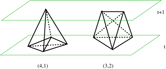
Figure 1: A triangulation in CDT consists of four-dimensional triangulated layers assembled from (4,1)- and (3,2)-simplices, interpolating between adjacent integer constant-time slices (left), which in turn are triangulations of $S^{3}$ in terms of equilateral tetrahedra. Each purely spatial tetrahedron at time $t$ forms the interface between two (4,1)-simplices, one in the interval $[t-1,1]$, and the other in $[t,t+1]$, as illustrated on the right. Although a (3,2)-simplex shares none of the five tetrahedra on its surface with a constant-time slice (the tetrahedra are all Lorentzian), it is nevertheless needed in addition to the (4,1)-building block to obtain simplicial manifolds with a well-defined causal structure.

The CDT lattice regularization differs in a crucial way from the DT lattice regularization discussed in the Introduction. While it uses the same action (the discretized Einstein-Hilbert action, in the form of the so-called Regge action[9]) as DT, it uses only triangulated manifolds with the topology of a direct product $[0,1]\times{}^{3}\Sigma$, and subject to a preferred proper-time foliation in the time direction. The motivation for this is twofold. While DT is inherently Euclidean in its set-up, CDT is an attempt to define the regularized path integral in spacetimes with Lorentzian signature. Following earlier ideas[10] we insist on including in the path integral only locally causal geometries, whose light cone structure is everywhere non-degenerate. CDT is an attempt to implement such a path integral, defined as a lattice regularization, much in the same way as was done using DT. (We refer the reader to a comprehensive recent review [11] for details.) Like the DT geometries, the CDT geometries are piecewise linear geometries constructed by gluing together a few standard building blocks, but such that they respect the proper-time foliation. In this construction we have space-like lattice links, to which we assign a length $ds^{2}=a_{s}^{2}=a^{2}$, and time-like lattice links, to which we assign a proper-time length $ds^{2}=a^{2}_{t}=-\alpha a^{2}$, where $a$ and $a_{s}$ are positive. This is illustrated in Fig. 1 in the case of four-dimensional spacetime, where four standard building blocks are needed, the so-called (4,1)- and (3,2)-building blocks shown in the figure and time-reversed (1,4)- and (2,3)-building blocks, the numbers referring to the number of vertices of the four-dimensional simplex at spatial slice $t$ and spatial slice $t+1$. The spatial slice at any $t$ is assumed to have the topology ${}^{3}\Sigma=S^{3}$ (we assume that space is compact, and have chosen the simplest topology), and is triangulated in terms of equilateral tetrahedra of link length $a_{s}$. At discrete times $t$ and $t+1$ we thus have two purely spatial triangulations of $S^{3}$. Fig. 1 illustrates how to fill in the four-dimensional “slab” between the two $S^{3}$-triangulations with four-simplices, preserving the topology $[0,1]\times S^{3}$. In the path integral we will sum over all triangulations of the three-sphere at $t$, all triangulations of the three-sphere at $t+1$, etc., and over all four-dimensional triangulations of the slabs compatible with the given choices of the spherical triangulations at $t$, $t+1$, $\dots$ . For each spacetime geometry thus obtained we can perform a rotation to Euclidean signature by rotating $\alpha$ from positive to negative values in the lower-half complex plane. The corresponding Regge action also rotates in the way expected for a rotation from Lorentzian to Euclidean signature, that is,

$$iS_{L}(\alpha)=-S_{E}(-\alpha).$$ (3)

The constraint of local causality is not a topological constraint, and after rotation to Euclidean signature leads to a summation over a restricted class of Euclidean geometries. The corresponding theory is therefore potentially different from “Euclidean quantum gravity” à la Hawking. This brings us to the second motivation for replacing the DT with the CDT regularization in spacetime dimensions $d$ larger than two. If one restricts oneself to the Euclidean Einstein-Hilbert action in Regge form, the DT lattice theory has no continuum limit. Studying the theory with Monte Carlo simulations, one finds a phase transition as a function of the bare gravitational coupling constant, but it is of first order. Such a first-order transition cannot be used to define a continuum quantum field theory. As discussed in the Introduction, we need a second-order transition to which we can associate a divergent correlation length. The situation will be different when we use the CDT regularization.

3 CDT phase structure

We will discuss here the four-dimensional CDT theory. We rotate it to Euclidean signature as described above. Because the four-dimensional theory cannot be solved analytically, we need to rotate it to Euclidean signature to be able to study it by Monte Carlo simulations.

Let us first write down the regularized Euclidean Einstein-Hilbert action for a CDT configuration. As mentioned earlier, we use the so-called Regge action, which can be used for any piecewise linear geometry. For a $d$-dimensional triangulation the curvature will be located at the $(d-2)$-dimensional subsimplices, which implies that in four dimensions the curvature is concentrated at the two-dimensional subsimplices (the triangles). In the case of CDT the Regge action becomes exceedingly simple, because we are using fixed building blocks to construct the geometries. The curvature depends only on how we glue these building blocks together. After using various identities relating the number of subsimplices and the order of vertices, links and triangles, the action will only depend on the total number $N_{0}$ of vertices, the total numbers $N_{4}^{(4,1)}$ and $N_{4}^{(3,2)}$ of (4,1)- and (3,2)-simplices and the parameter $\alpha$,

$$S_{E}[-\alpha;T] = -(\kappa_{0}+6\Delta)N_{0}(T)+\kappa_{4}\Big{(}N_{4}^{(3,2)}(T)+N_{4}^{(4,1)}(T)\Big{)}$$

$$+\Delta\Big{(}N_{4}^{(3,2)}(T)+2N_{4}^{(4,1)}(T)\Big{)},$$

where the asymmetry parameter $\Delta$ is a function of $\alpha$ such that $\Delta(\alpha\!=\!1)=0$. In this formula $\kappa_{0}\propto 1/G_{0}$, the bare inverse gravitational coupling constant, while $\kappa_{4}$ can be more or less identified with $\Lambda_{0}/G_{0}$, $\Lambda_{0}$ being the bare cosmological coupling constant. The CDT partition function is given by

$$Z(\kappa_{0},\kappa_{4},\Delta)=\sum_{T}\mbox{e}^{-S_{E}[T]},$$ (5)

where one sums over four-dimensional CDT triangulations of the kind described in the previous Section. We should point out that formula (5) contains a small subtlety. In the first place, one would not consider $\Delta$ as a coupling constant. It was merely chosen to parametrize the asymmetry between the links in spatial and temporal directions, but the classical Einstein-Hilbert action was adjusted precisely to take this into account. However, it turns out that in the region of bare coupling-constant space where we observe a potentially interesting phase structure, the entropy of configurations with the same action is as important as the action itself. Although the entropy is independent of $\Delta$, the real quantum effective action becomes in this way a function of $\Delta$. In the classical limit the contribution of the (bare) action will always be much more important than the entropy term, simply because the action is multiplied by $1/\hbar$, while this is not the case for the entropy term. However, the interesting Planckian physics we observe is of course not in this semiclassical limit. It follows that we have a theory depending on three coupling constants, $\kappa_{0}$, $\kappa_{4}$ and $\Delta$. For technical convenience, we keep the four-volume fixed during the Monte Carlo simulations, which effectively removes $\kappa_{4}$ as a coupling constant. We are thus left with two coupling constants, $\kappa_{0}$ and $\Delta$.

The numerical set-up is as follows: we choose a four-volume (the discrete number of four-simplices) and a large proper-time extent $t$ (the discrete number of lattice time steps), and perform the Monte Carlo simulations for a given choice of $\kappa_{0}$ and $\Delta$. We can measure the three-volume distribution as a function of proper time $t^{\prime}$ between 0 and $t$, and deduce from the measurements that there are three qualitatively different types of three-volume profiles $N_{3}(t^{\prime})$, depending on the choice of $\kappa_{0}$ and $\Delta$. Here $N_{3}(t^{\prime})$ denotes the number of tetrahedra forming a triangulation of the spatial slice at time $t^{\prime}$. The different profiles correspond to different phases, which we have denoted by A, B and C [12]. The corresponding phase diagram is shown in Fig. 2 (we refer to elsewhere[13] for details).

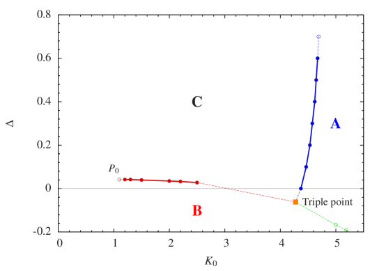
Figure 2: The phase diagram of four-dimensional CDT.

In phase B we observe a collapse of the four-dimensional universe to a three-dimension one, in the sense that all of the three-volume $N_{3}(t^{\prime})$, $t^{\prime}\in[0,t]$, is located at a single time. The situation in phase A is completely opposite. The three-volume $N_{3}(t^{\prime})$ is spread out over the whole time interval $[0,t]$, and the magnitude of $N_{3}(t^{\prime})$ is close to being a random variable, with little correlation with the neighbouring three-volumes $N_{3}(t^{\prime}+1)$ and $N_{3}(t^{\prime}-1)$ (at least, the correlation is rather short-ranged). Finally, in phase C the situation is again very different. There is no collapse of three-volume around a single spatial slice. Instead, the three-volumes $N_{3}(t^{\prime})$ at adjacent times are highly correlated, resulting in a genuinely four-dimensional universe. The universe has a definite extension in the time direction, independent of the choice of $t$, as long as $t$ is sufficiently large compared to the given choice of $N_{4}$. Along the remainder of the $t$-axis one finds only vanishing three-volume (to be precise, one finds three-volumes which are close to the minimal cut-off size of 5 tetrahedra, since we do not allow the computer algorithm to shrink the three-volume to strictly zero). The actual time extension of the universe depends on the chosen $N_{4}$ and scales proportional to $N_{4}^{1/4}$ as one would naïvely expect. Similarly, the non-zero three-volumes $N_{3}(t^{\prime})$ scale proportional to $N_{4}^{3/4}$. This is the reason why we claim that the universe is four-dimensional[12]. At first sight it may seem a triviality that the universe should scale in this fashion, but it is in fact highly non-trivial. Although the elementary building blocks are four-dimensional, nothing tells us that they will line up to form a four-dimensional object with approximately $N_{4}^{1/4}$ building blocks in each direction. Since absolutely no “background” geometry has been put in by hand to ensure the four-dimensionality of the resulting “quantum spacetime”, this will in general not happen at any scale, as exemplified by the situation in phases A and B. Furthermore, as we have already noted and as will be discussed later, in phase C we are far from any choice of the bare coupling constants where the classical action dominates.

We thus have identified three phases with very different geometric large-scale characteristics. Associated with these phases are phase transition lines, as shown in Fig. 2. We have investigated the order of these transitions, with the result that the transition A-C is first order, while the transition B-C is second order[14]. (We are currently not particularly interested in the transition A-B, since geometry in neither phase A nor B seems relevant as a model for a four-dimensional universe.)

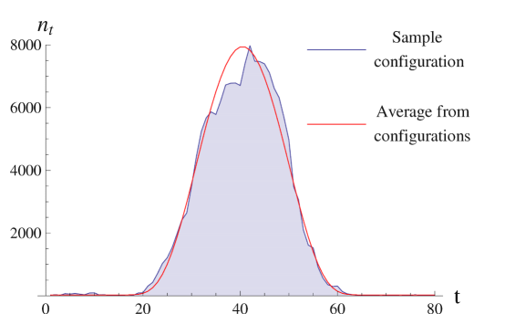
Figure 3: A typical three-volume profile (and the average profile) for some choice of coupling constants in phase C.

Following the Wilsonian logic on how to take the continuum limit, our main interest will be focused on the B-C phase transition line. Can it be used to define a UV limit of quantum gravity? Before addressing this point, we will take a closer look at the situation in phase C, where we seemingly observe four-dimensional universes.

4 The physics of phase C

A typical three-volume profile in phase C is shown in Fig. 3. Fig. 4 highlights the average value of the profile and the size of typical fluctuations. The data are collected for fixed values of the coupling constants and fixed $N_{4}$. For the average profile there is a perfect scaling $\propto N_{4}^{3/4}$ of the height and $\propto N_{4}^{1/4}$ of the width of the profile. However, the fluctuations of the height of the profile scale like $N_{4}^{1/2}$. This means that for fixed values of the bare coupling constants, taking $N_{4}\to\infty$, the relative fluctuations will go to zero and we will have a well-defined limit. For fixed values of the bare coupling constants, the average profile can be fitted perfectly to the formula

$$\langle N_{3}(i)\rangle\propto N_{4}^{{3}/{4}}\cos^{3}\left(\frac{i}{s_{0}N_{4}^{1/4}}\right),$$ (6)

where $i$ denotes (integer) lattice time, $N_{4}$ the total number of four-simplices and $N_{3}(i)$ the number of tetrahedra at time $i$ [15], and $s_{0}$ is a constant which will depend on the choice of bare coupling constants (the formula is of course not valid in the “stalk”, where $N_{3}(i)\approx 5$.).

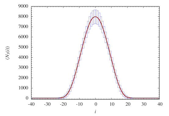
Figure 4: The average three-volume profile and the fluctuations for $N_{4}=360.000$, at $\kappa_{0}=2.2$ and $\Delta=0.6$.

Can the functional form of the expectation value found in (6) be obtained directly from an action principle? The answer is yes [16]. The minisuperspace approach to quantum gravity by Hartle and Hawking[17], which only involves the scale factor of the universe (equivalently, the three-volume) reduces the Einstein-Hilbert action to the “effective” action

$$S_{\mathit{e}f\!f}=-\frac{1}{24\pi G}\int dt\left(\frac{\dot{V_{3}}^{2}(t)}{V_{3}(t)}+k_{2}V_{3}^{1/3}(t)-\lambda V_{3}(t)\right),$$ (7)

where $t$ denotes proper time, $k_{2}$ is a numerical constant and $\lambda$ is a Lagrange multiplier (not a cosmological constant), because the total four-volume $V_{4}$ is kept fixed in the simulations. The classical solution of the equations of motion corresponding to $S_{ef\!f}$ is precisely the $\cos^{3}(t/V_{4}^{1/4})$ referred to in eq. (6).

From the computer simulations and the measurements of $\langle N_{3}(i)\rangle$ and $\langle N_{3}(i)N_{3}(j)\rangle$ it is possible to reconstruct the effective discretized action leading to (6). It has the form[15]

$$S_{discr}=k_{1}\sum_{i}\left(\frac{(N_{3}(i+1)-N_{3}(i))^{2}}{N_{3}(i)}+\tilde{k}_{2}N_{3}^{1/3}(i)-\tilde{\lambda}N_{3}(i)\right).$$ (8)

This is precisely the discretized version of (7), except for an overall sign. This overall sign does not affect the equations of motion derived from the actions, but it shows that in phase C we are far away from any semiclassical limit, even if the effective outcome (the average universe) is similar. Since the effective action (8) comes from combining the discretized, bare Einstein-Hilbert action and the entropy of configurations, as discussed earlier, it is clear that entropy plays an important role in phase C.

Finally, from the effective action (8), and comparing to (7), it is natural to consider $k_{1}$, which we can actually measure, as the dimensionless coupling constant

$$k_{1}\propto a^{2}/G(a),$$ (9)

where we have assumed a scale-dependence of the gravitational coupling constant $G$, using as scale parameter the lattice cut-off $a$. In the asymptotic safety scenario, $k_{1}$ should run to a constant different from zero when we approach a non-trivial UV fixed point, while it should go to zero in the IR, where $G(a)\to G$, the ordinary gravitational coupling constant. We have measured $k_{1}(\kappa_{0},\Delta)$, and there is a clear indication that it goes to zero when we keep $\Delta$ fixed and increase $\kappa_{0}$, moving in phase C towards phase $A$. Similarly, there is some evidence that $k_{1}(\kappa_{0},\Delta)$ does not go to zero when we approach the B-C phase transition line moving in phase C, keeping $\kappa_{0}$ constant while decreasing $\Delta$. This points to the B-C line being associated with UV physics. We will now discuss this further by studying lines of constant physics in phase C.

5 Renormalization group flow

The renormalization group equation in terms of the dimensionless gravitational coupling constant ${\hat{G}}(a)\propto 1/k_{1}(a)$ reads

$$G(a)=a^{2}{\hat{G}}(a),~{}~{}~{}~{}a\frac{\mbox{d}{\hat{G}}}{\mbox{d}a}=-\beta({\hat{G}}),~{}~{}~{}~{}\beta({\hat{G}})=2{\hat{G}}-c{\hat{G}}^{2}+\dots\;.$$ (10)

The $\beta$-function is assumed to have a non-trivial zero (if we ignore the dots, which signify higher-order contributions, it is at ${\hat{G}}^{*}=2/c$). Close to the fixed point we can write

$${\hat{G}}(a)={\hat{G}}^{*}-Ka^{\tilde{c}},~{}~{}~{}k_{1}(a)=k_{1}^{*}+\tilde{K}a^{\tilde{c}},$$ (11)

for some $K$, $\tilde{K}$, where the approach to the fixed point is governed by the exponent

$${\tilde{c}}=-\beta^{\prime}({\hat{G}}^{*}).$$ (12)

In a standard lattice theory one would now relate the lattice spacing near the fixed point to the bare coupling constants with the help of some correlation length $\xi$. As we have already discussed, the concept of a correlation length makes perfect sense even in a theory of fluctuating geometries (see eq. (2) for a definition of a diffeomorphism-invariant correlator). Having such a correlation length available would allow us to define a path of constant physics when we change the bare coupling constant (denoted by $g_{0}$), namely, by insisting that the correlation length $\xi(g_{0})$, expressed as the number of lattice spacings times the lattice length $a$, represents a physical length, which is constant when we approach the fixed point $g_{0}^{*}$ where $\xi(g_{0})$ diverges. Typically one has

$$\xi(g_{0})=\frac{c}{|g_{0}-g_{0}^{*}|^{\nu}},~{}~{}~{}{\rm i.e.}~{}~{}~{}a(g_{0})\propto|g_{0}-g_{0}^{*}|^{\nu},$$ (13)

thus determining how we should scale the lattice spacing to zero as a function of the bare coupling constant $g_{0}$. However, in four-dimensional quantum gravity without matter we do not yet have a suitable correlation length at our disposal which could play this role. In search of an alternative, let us first consider the equation $V_{4}=N_{4}a^{4}$, which defines the dimensionful continuum four-volume $V_{4}$ in terms of the number $N_{4}$ of four-simplices and the lattice spacing. If we could consider $V_{4}$ as fixed, we could replace the $a$-dependence of (11) by a $N_{4}$-dependence, with the advantage that $N_{4}$ is a parameter we can straightforwardly control. Re-expressing eq. (11) in terms of $N_{4}$ yields

$$k_{1}(N_{4})=k_{1}^{*}-K^{\prime}N_{4}^{-{\tilde{c}}/4},$$ (14)

for some $K^{\prime}$. Since we can measure $k_{1}$, we could determine the flow to the fixed point.

In order to apply (14), we need to ensure that we can consider $V_{4}$ as fixed when we change $N_{4}$. For each value of coupling constants and each value $N_{4}$ one has a three-volume profile like the one shown in Fig. 4. Let us be more specific and rewrite (6) as

$$N_{3}(i)=\frac{3}{4\omega}{\tilde{N}}_{4}^{3/4}\cos^{3}\left(\frac{i}{\omega{\tilde{N}}_{4}^{1/4}}\right),$$ (15)

and for the fluctuations

$$\delta N_{3}(i)=\gamma{\tilde{N}}_{4}^{1/2}F\left(\frac{i}{\omega{\tilde{N}}_{4}^{1/4}}\right),$$ (16)

where ${\tilde{N}}_{4}$ is the number of four-simplices of type (4,1) (and by construction the total number of tetrahedra contained in the spatial slices), and where $F(t)$ is a function we have measured[15]. ${\tilde{N}}_{4}$ is on average proportional to the total number of four-simplices, the constant of proportionality depending somewhat on the choice of bare coupling constants, as already noted. $\gamma$ and $\omega$ depend on the bare coupling constants $\kappa_{0}$ and $\Delta$. We can now write

$$\frac{\delta N_{3}(i)}{N_{3}(i)}=\frac{4\gamma\omega}{3{\tilde{N}}_{4}^{1/4}}\;\left(\frac{F(i/(\omega{\tilde{N}}_{4}^{1/4}))}{\cos^{3}(i/(\omega{\tilde{N}}_{4}^{1/4}))}\right).$$ (17)

Well away from the phase transition boundaries, our measurements show that $\omega$ and $\gamma$ are independent of ${\tilde{N}}_{4}$, when ${\tilde{N}}_{4}$ is not too small. Thus, increasing ${\tilde{N}}_{4}$ while staying at a specific point $(\kappa_{0},\Delta)$ in phase C does not correspond to keeping $V_{4}$ fixed, because during this process the size of the quantum fluctuations in the three-volume decreases relative to the expectation value of the three-volume according to

$$\frac{\delta N_{3}}{N_{3}}\propto\frac{1}{{\tilde{N}}_{4}^{1/4}}.$$ (18)

It is a reasonable requirement for a continuum limit that the ratio (17) be independent of ${\tilde{N}}_{4}$ for fixed $i/(\omega{\tilde{N}}_{4}^{1/4})$. Thus, if we start at a given ${\tilde{N}}_{4}^{(0)}$, using coupling constants $\kappa_{0}(0)$ and $\Delta(0)$, and change ${\tilde{N}}_{4}$, we have to change $\kappa_{0}$ and $\Delta$ such that

$$\gamma(\kappa_{0},\Delta)\,\omega(\kappa_{0},\Delta)=\gamma(\kappa_{0}(0),\Delta(0))\,\omega(\kappa_{0}(0),\Delta(0))\;\frac{{\tilde{N}}_{4}^{1/4}}{({\tilde{N}}_{4}^{(0)})^{1/4}}$$ (19)

holds. We can measure $\omega(\kappa_{0},\Delta)$ and $\gamma(\kappa_{0},\Delta)$ in phase C, and have done so, but eq. (19) is not sufficient to determine a curve $(\kappa_{0}({\tilde{N}}_{4}),\Delta({\tilde{N}}_{4})$. We need another condition. It is tempting to choose as a second condition that $\omega(\kappa_{0},\Delta)$ stay constant along a curve of constant $V_{4}$. This requirement implies according to (15) that all three-volume profiles along the curve can be scaled to coincide by identical scaling in “time” and “space” directions, something which is compatible with our intuitive understanding of what it means to have constant $V_{4}$. The requirement that $\omega(\kappa_{0},\Delta)=\omega(\kappa_{0}(0),\Delta(0))$ determines a curve starting at $(\kappa_{0}(0),\Delta(0))$. Moving along this curve, eq. (19) determines the relationship between $\gamma$ and ${\tilde{N}}_{4}$ according to

$$\gamma(\kappa_{0}({\tilde{N}}_{4}),\Delta({\tilde{N}}_{4}))=\gamma(\kappa_{0}(0),\Delta(0))\;\frac{{\tilde{N}}_{4}^{1/4}}{({\tilde{N}}_{4}^{(0)})^{1/4}},$$ (20)

provided it can be satisfied.

In Fig. (5) we show the lines of constant $\omega$ as functions of $\kappa_{0}$ and $\Delta$, superimposed on a contour plot of $\gamma(\kappa_{0},\Delta)$. If we start out some distance from the B-C phase boundary, the plot indicates that it is impossible to flow to the B-C transition line along lines of constant $\omega$ with increasing ${\tilde{N}}_{4}$.

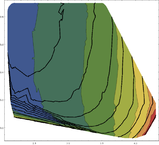
Figure 5: The flow diagram in phase C. The flow lines correspond to constant $\omega$ in eq. (15) (black lines). The contour plot refers to the change of $\gamma$ ($\gamma$ increases going from the blue to the red region).

However, the situation changes as we move closer to the B-C phase transition line. The lines of constant $\omega$ now seem to be directed towards the triple point. In addition, the increase of $\gamma$ is maximal when we move in the same direction towards the triple point. Thus there is the tantalizing possibility that we can have paths of constant physics leading to the triple point, with (20) satisfied when moving along the path.

While the condition $\omega=const.$ may seem a reasonable requirement to impose for constant $V_{4}$, we are not forced to adopt it. One can even argue that one should not use it. The reason is that $\omega$ changes as a function of the bare coupling constants $\kappa_{0}$ and $\Delta$. Its main dependence is on $\Delta$, and $\omega$ goes to zero when we approach the B-C phase transition line by decreasing $\Delta$ (within measuring accuracy). We thus have two options: if we regard the change in $\omega$ as reflecting a change in our universe, the universe contracts in the time direction when we approach the B-C line. In order to obtain a finite continuum time extent at the transition line one may therefore have to scale time and space with different powers of the cut-off $a$ when approaching the B-C line. This leads naturally to a Hořava-Lifshitz scenario, which we will discuss in the next Section.

Alternatively, one could adopt the viewpoint that all universes of the form (15) can be identified if we are allowed to rescale time relative to space by some constant that depends on the bare coupling constants. Such a freedom implies that we are not taking literally the microscopic identification of proper time as the number of lattice steps in the “time” direction times $a_{t}$, the lattice spacing in the time direction, but only claim that it is proportional to the “real” proper time. Thus we are not forced to take a path of constant $\omega$ to consider $V_{4}$ constant. However, as mentioned above, it leaves us short of one condition if we want to determine a path in the coupling constant space corresponding to what we call constant $V_{4}$.

6 Relation to Hořava-Lifshitz gravity

As we have described above, CDT provides a non-perturbative lattice regularization for a quantum theory of geometries, characterized by the presence of a preferred time foliation. In the Euclidean sector one can prove that the lattice theory has a transfer matrix which is reflection-positive[7]. One would therefore expect that a continuum theory obtained from the lattice theory will have a unitary time evolution.

The features just mentioned resemble those imposed in Hořava-Lifshitz gravity [5]. This suggests that CDT can provide a lattice regularization of quantum Hořava-Lifshitz gravity. Indeed, in the simplest case of two space-time dimensions, one can prove that CDT coincides with so-called quantum projectable HL gravity [19] with at most quadratic derivative terms. Of course, the situation in two dimensions is rather special. Although 1+1 dimensional CDT has a preferred time foliation, it is related to standard two-dimensional Euclidean quantum gravity (Liouville quantum gravity) in a simple way [6, 20]. CDT is the “effective” theory obtained from Liouville quantum gravity by integrating out all Liouville quantum gravity “baby universes”. As a consequence, the amplitudes of the two theories are related by a simple (non-analytic) mapping between their respective coupling constants.

In higher dimensions, Hořava’s idea was to introduce higher-derivative terms in the spatial directions to render the theory renormalizable, while having only second-order time derivatives to ensure unitarity. Unlike HL gravity, CDT does not introduce explicit higher-order derivative terms in the spatial directions. However, as already mentioned, since entropic terms are important, it may be that such higher-derivative terms are present in the effective CDT action. It is conceivable that for some choices of bare coupling constants CDT provides us with a regularization of quantum general relativity, while for others it is a regularization of quantum HL gravity.

The CDT phase diagram presented in Fig. 2 has a striking similarity to a Lifshitz phase diagram, as noticed already elsewhere[13, 21]. Even the characteristics of the phases A, B and C can be described in a language similar to the one used for a magnetic Lifshitz system (details can be found in earlier work [13]).

When we move towards the second-order phase transition line B-C, we observe a contraction of the quantum universe in the time direction. This is in agreement with the fact that we have a second-order transition and that the universe in phase B collapses to a single time slice. It indicates that in order to obtain a genuine continuum limit when approaching the B-C line, one may have to scale time and space differently, a characteristic feature of HL gravity too. Various possible isotropic and anisotropic relations between space and time have been discussed [13].

Can the average quantum universe we observe on the computer be understood as a HL universe rather than a universe coming from the effective GR minisuperspace action (7)? In the context of HL gravity, one can also derive a minisuperspace action[22], namely,

$$S_{mini}=\frac{2\pi^{2}}{16\pi G}\int\mbox{d}t\;a(t)^{3}\Big{(}3(1-3\lambda)\ \frac{\dot{a}^{2}}{a^{2}}-\gamma\ \frac{6}{a^{2}}+2\Lambda+{\tilde{V}}(a)\Big{)},$$ (21)

where we have used the scale factor $a(t)$ instead of $V(t)\propto a(t)^{3}$. The parameters $\lambda$ and $\gamma$ are equal to 1 in the case of ordinary general relativity, but can be different from 1 in HL gravity, and define the IR limit of HL gravity. The potential ${\tilde{V}}(a)$ contains inverse powers of the scale factor $a$ coming from possible higher-order spatial derivative terms.

Our reconstruction of the effective action from the computer data is compatible with the functional form (21) of the minisuperspace action. If we were able to extract the constant $\tilde{k}_{2}$ in front of the potential term in (8), it would enable us to fix the ratio $(1-3\lambda)/2\gamma$ appearing in (21) [15, 23]. At this stage, the precision of our measurements is insufficient to do so. The same is true for our attempts to determine ${\tilde{V}}(a)$ for small values of the scale factor, which is important for understanding UV quantum corrections to the potential near $a(t)=0$.

7 Summary

CDT was born as an attempt to formulate a non-perturbative path integral directly in spacetimes with Lorentzian signature. It can be rotated explicitly to Euclidean signature, a necessity if one wants to use Monte Carlo simulations to study the non-perturbatively defined theory of fluctuating geometries. Like the ADM formalism, the Lorentzian formulation introduces an asymmetry between space and time. This asymmetry survives after rotation to Euclidean signature, and can potentially make the theory different from so-called Euclidean quantum gravity. CDT rotated to Euclidean signature has a positive definite transfer matrix and thus a unitary time evolution when the theory is rotated back to Lorentzian time. Both the set-up with a preferred (proper) time and the resulting unitarity are reminiscent of the starting point of HL gravity in the continuum. The CDT formalism can be used as regularization of a quantum HL gravity theory, something which has already been done successfully in 2+1 dimensions [24]. Our original goal was to provide a non-perturbative regularization of GR, as a possible realization (and truly non-perturbative verification) of the asymptotic safety scenario. For this reason we have never added higher-order spatial derivative terms to the bare action, as is done in HL gravity, but such terms could in principle be created by the entropy factor. The phase diagram we observe is quite similar to a Lifshitz diagram, indicating that an interpretation in terms of HL gravity may be natural. An appealing possibility is that our approach includes both scenarios, where the asymptotic safety scenario with full GR invariance may correspond to a special choice of bare coupling constants, i.e. a fine-tuning of the relation between the Regge action and the entropy term in the effective quantum action. Better data and more observables will be required to discriminate between a “pure gravity” behaviour and an anisotropic deformation à la Hořava-Lifshitz in the deep ultraviolet.

Acknowledgment

JA and AG thank the Danish Research Council for financial support via the grant ”Quantum gravity and the role of black holes”, and the EU for support through the ERC Advanced Grant 291092, ”Exploring the Quantum Universe” (EQU). JJ acknowledges partial support through the International PhD Projects Programme of the Foundation for Polish Science within the European Regional Development Fund of the European Union, agreement no. MPD/2009/6. RL acknowledges support through several Projectruimte grants by the Dutch Foundation for Fundamental Research on Matter (FOM). The contributions of JA and RL were supported in part by the Perimeter Institute of Theoretical Physics. Research at Perimeter Institute is supported by the Government of Canada through Industry Canada and by the Province of Ontario through the Ministry of Economic Development & Innovation.

References

- [1] Approaches to quantum gravity, ed. D. Oriti (Cambridge University Press, UK, 2009).
- [2] S. Weinberg, in General relativity: Einstein centenary survey, eds. S.W. Hawking and W. Israel (Cambridge University Press, UK, 1979) 790-831.
-
[3]
M. Reuter,
Phys. Rev. D 57 971-985 (1998);
A. Codello, R. Percacci and C. Rahmede, Annals Phys. 324 414 (2009);
M. Reuter and F. Saueressig, arXiv:0708.1317;
M. Niedermaier and M. Reuter, Living Rev. Rel. 9 5 (2006) 5;
H.W. Hamber and R.M. Williams, Phys. Rev. D 72 044026 (2005);
D.F. Litim, Phys. Rev. Lett. 92 20130 (2004). -
[4]
H. Kawai and M. Ninomiya,
Nucl. Phys. B 336 115 (1990);
H. Kawai, Y. Kitazawa and M. Ninomiya, Nucl. Phys. B 393 280-300 (1993);
Nucl. Phys. B 404 684-716 (1993); Nucl. Phys. B 467 313-331 (1996);
T. Aida, Y. Kitazawa, H. Kawai and M. Ninomiya, Nucl. Phys. B 427 158-180 (1994). -
[5]
P. Hořava,
Phys. Rev. D 79 084008 (2009);
P. Hořava and C.M. Melby-Thompson, Phys. Rev. D 82 064027 (2010). - [6] J. Ambjørn and R. Loll, Nucl. Phys. B 536 407-434 (1998).
- [7] J. Ambjørn, J. Jurkiewicz and R. Loll, Nucl. Phys. B 610 347-382 (2001); Phys. Rev. Lett. 85 924 (2000).
-
[8]
J. Ambjørn and K.N. Anagnostopoulos,
Nucl. Phys. B 497 445 (1997);
J. Ambjørn, K.N. Anagnostopoulos, U. Magnea and G. Thorleifsson, Phys. Lett. B 388 713 (1996);
J. Ambjørn, J. Jurkiewicz and Y. Watabiki, Nucl. Phys. B 454 313-342 (1995); J. Ambjørn and Y. Watabiki, Nucl. Phys. B 445 129 (1995). - [9] T. Regge, Nuovo Cim. 19 558 (1961).
-
[10]
C. Teitelboim,
Phys. Rev. Lett. 50 (1983) 705-708;
Phys. Rev. D 28 (1983) 297-309. - [11] J. Ambjørn, A. Görlich, J. Jurkiewicz, R. Loll, Phys. Rep. 519 (2012) 127-210, arXiv:1203.3591.
- [12] J. Ambjørn, J. Jurkiewicz and R. Loll, Phys. Rev. Lett. 93 131301 (2004); Phys. Rev. D 72 064014 (2005).
- [13] J. Ambjørn, A. Görlich, S. Jordan, J. Jurkiewicz and R. Loll, Phys. Lett. B 690 413-419 (2010) 413-419.
- [14] J. Ambjørn, S. Jordan, J. Jurkiewicz and R. Loll, Phys. Rev. Lett. 107 211303 (2011); Phys. Rev. D 85 124044 (2012).
- [15] J. Ambjørn, A. Görlich, J. Jurkiewicz and R. Loll, Phys. Rev. Lett. 100 091304 (2008); Phys. Rev. D 78 063544 (2008).
- [16] J. Ambjørn, J. Jurkiewicz and R. Loll, Phys. Lett. B 607 205-213 (2005).
- [17] J.B. Hartle and S.W. Hawking, Phys. Rev. D 28 2960-2975 (1983).
- [18] S. Jordan and R. Loll, Causal Dynamical Triangulations without preferred foliation, arXiv:1305.4582.
- [19] J. Ambjørn, L. Glaser, Y. Sato and Y. Watabiki, 2d CDT is 2d Horava-Lifshitz quantum gravity, arXiv:1302.6359.
- [20] J. Ambjørn, J. Correia, C. Kristjansen and R. Loll, Phys. Lett. B 475 24-32 (2000).
- [21] P. Hořava, Class. Quant. Grav. 28 (2011) 114012, arXiv:1101.1081.
-
[22]
E. Kiritsis and G. Kofinas,
Nucl. Phys. B 821 467 (2009) 467;
R. Brandenberger, Phys. Rev. D 80 043516 (2009);
G. Calcagni, JHEP 0909 112 (2009). - [23] J. Ambjørn, A. Gorlich, J. Jurkiewicz, R. Loll, J. Gizbert-Studnicki and T. Trzesniewski, Nucl. Phys. B 849 144 (2011).
- [24] C. Anderson, S. J. Carlip, J. H. Cooperman, P. Horava, R. K. Kommu and P. R. Zulkowski, Phys. Rev. D 85 044027 (2012).