Langevin dynamics in inhomogeneous media: Re-examining the Itô-Stratonovich Dilemma

Abstract

The diffusive dynamics of a particle in a medium with space-dependent friction coefficient is studied within the framework of the inertial Langevin equation. In this description, the ambiguous interpretation of the stochastic integral, known as the Itô-Stratonovich dilemma, is avoided since all interpretations converge to the same solution in the limit of small time steps. We use a newly developed method for Langevin simulations to measure the probability distribution of a particle diffusing in a flat potential. Our results reveal that both the Itô and Stratonovich interpretations converge very slowly to the uniform equilibrium distribution for vanishing time step sizes. Three other conventions exhibit significantly improved accuracy: (i) the “isothermal” (Hänggi) convention, (ii) the Stratonovich convention corrected by a drift term, and (iii) a new convention employing two different effective friction coefficients representing two different averages of the friction function during the time step. We argue that the most physically accurate dynamical description is provided by the third convention, in which the particle experiences a drift originating from the dissipation instead of the fluctuation term. This feature is directly related to the fact that the drift is a result of an inertial effect that cannot be well understood in the Brownian, overdamped limit of the Langevin equation.

I Introduction

The dynamics of a particle coupled to a thermal heat bath is traditionally described by the Langevin equation of motion. Denoting the position and velocity of the particle at time $t$ by $r(t)$ and $v(t)=\dot{r}$, respectively, the Langevin equation reads coffey

$$m\dot{v} = f(r,t)-\alpha v+\beta(t),$$ (1)

where $m$ is the mass of the particle. This is Newtonian dynamics for which the applied force is described as a composite of three kinds: (i) deterministic forces $f(r,t)$, (ii) a friction force $-\alpha v$ proportional to the velocity with friction coefficient $\alpha\geq 0$, and (iii) a stochastic force $\beta(t)$ representing fluctuations arising from interactions with the embedding medium that produces the friction. The stochastic force can be conveniently modeled by a delta-correlated (“white”) Gaussian noise with statistical properties: $\langle\beta(t)\rangle=0$ and $\langle\beta(t)\beta(t^{\prime})\rangle=2\alpha k_{B}T\delta(t-t^{\prime})$, where $k_{B}$ is Boltzmann’s constant and $T$ is the thermodynamic temperature parisi . This definitions ensure that, over large times, the position of the particle produces the Boltzmann distribution $\rho(r)\sim\exp[-U(r)/k_{B}T]$, where $f=-\nabla U(r)$, $U(r)$ being the potential energy surface kampen . Moreover, in the case of a flat potential (i.e., for $f=0$), the particle exhibits diffusive behavior with diffusion coefficient $D=k_{B}T/\alpha$ - in agreement with the fluctuation-dissipation theorem kubo

Implied in the above description is that the friction coefficient $\alpha$ is a constant. Now consider the particle diffusing in an inhomogeneous medium with position-dependent friction coefficient $\alpha(r)$. Presumably, the dynamics of a particle in such an environment is governed by Eq. (1), with the constant $\alpha$ simply replaced by the position-dependent $\alpha(r)$. This is formally correct, but physically meaningless, as readily becomes obvious when one attempts to calculate the particle trajectory by integrating Eq. (1) over a short time interval $dt$ doob . For a uniform $\alpha$, the integral over the stochastic noise is a well-defined Wiener process

$$\int_{0}^{dt}\beta(t^{\prime})\,dt^{\prime}=\sqrt{2\alpha k_{B}Tdt}\,\sigma,$$ (2)

where $\sigma$ is a standard Gaussian random number with $\langle\sigma\rangle=0$ and $\langle\sigma^{2}\rangle=1$ coffey ; kampen . For a non-uniform $\alpha(r)$, the integral is ill-defined, since one needs to specify at which point along the trajectory the friction coefficient in Eq. (2) is evaluated. This ambiguity is known as the Itô-Stratonovich dilemma coffey ; mannella . In Itô’s interpretation ito , the friction coefficient is taken at the beginning of the time step, while the Stratonovich interpretation considers the algebraic mean of the initial and final frictions stratonovich (which, for a small time interval, is very close to the friction at the mid-point). In the Brownian (overdamped) limit of the Langevin equation (i.e., when the left hand side of Eq. (1) vanishes), neither of these two interpretations reproduce the Boltzmann distribution. Instead, it is the the so called “isothermal” (Hänggi) convention hanggi , which takes the friction coefficient at the end of the time step, that generates the correct equilibrium statistics lau ; footnote .

Equilibrium statistics may also be acheived within the Itô or the Stratonovich formulation for Brownian dynamics. In these conventions, however, the associated Focker-Planck equation must be augmented with a “spurious” force term proportional to the gradient of the logarithm of the friction coefficient $f_{s}\sim-k_{B}T\alpha^{\prime}(r)/\alpha(r)$ lau ; volpe ; sancho (see further discussion in section IV on the “corrected Stratonovich convention” employing a spurious drift correction associated with this extra term). The necessity of such spurious force term can be understood through the following example tupper . Consider a Brownian particle diffusing between two immiscible fluids with a sharp interface between them. In the absence of an external potential, the equilibrium distribution is uniform, and the particle is expected, on average, to spend an equal amount time on both sides of the interface. However, this expectation appears to contradict the observation that the particle diffuses slower, and therefore becomes trapped, on the more viscous side. These conflicting arguments can be reconciled by assuming that there exists a boundary-force that pushes the particle toward the less viscous fluid. Thus, the particle has a smaller probability to enter the more viscous side in a manner that exactly cancels the trapping effect.

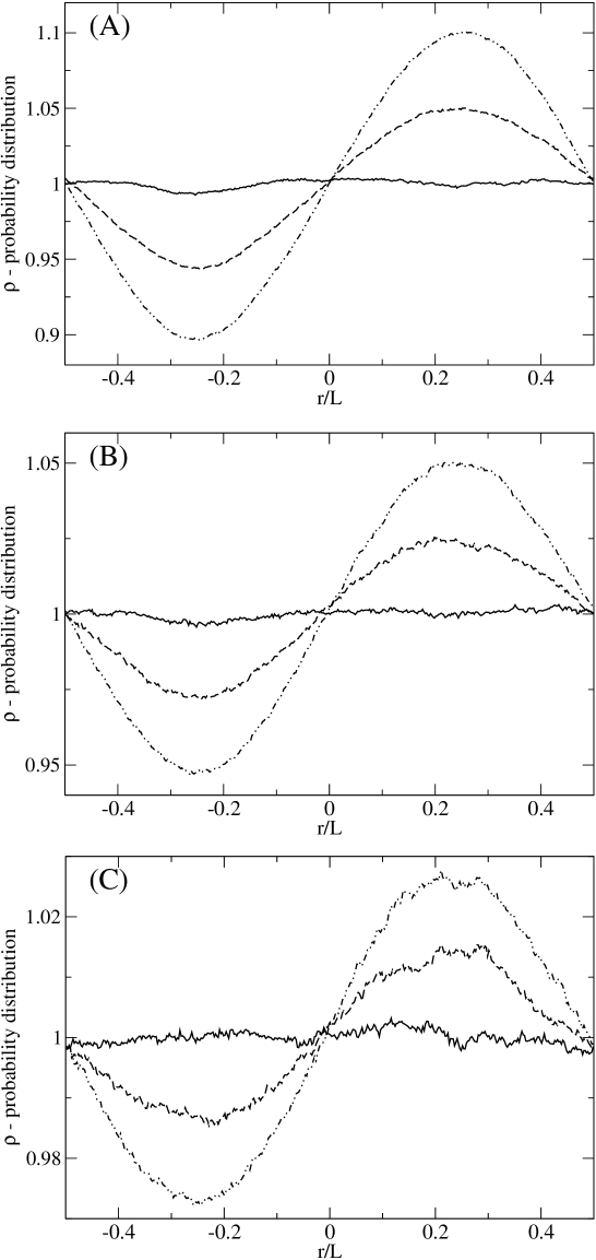
Figure 1: Probability distribution computed using Itô (dashed-dotted), Stratonovich (dashed), isothermal (solid line) conventions, for (A) $dt=0.1$, (B) $dt=0.05$, and (C) $dt=0.025$. Trajectories were generated using Eqs. (LABEL:pos-equation)-(LABEL:vel-equation), with $\bar{\alpha}_{r}=\bar{\alpha}_{t}=\alpha(r^{n})$ (Itô), $\bar{\alpha}_{r}=\bar{\alpha}_{t}=\int_{r^{n}}^{r^{n+1}}\!\!\!\!\alpha(r^{\prime})dr^{\prime}/(r^{n+1}-r^{n})$ (Stratonovich), $\bar{\alpha}_{r}=\bar{\alpha}_{t}=\alpha(r^{n+1})$ (isothermal).

So far there has been relatively little discussion of the Itô-Stratonovich dilemma in the framework of the full inertial Langevin equation. (Recent noticeable exceptions includes the treatment in Refs. sancho ; kupferman where the Brownian overdamped limit has been approached through “adiabatic elimination” of the inertial degrees of freedom.) This can be attributed to the less “catastrophic” consequences of the dilemma on the second order differential Langevin equation in comparison to the first order overdamped Brownian equation of motion. Suppose $r(t)$ is calculated by numerically integrating the equation of motion with $N$ small time steps of size $dt=t/N$. For the first order Brownian equation the velocity diverges, resulting in different results of $r(t)$ when applying different interpretations (Itô, Stratonovich, isothermal); even for $dt\rightarrow 0$ (see Ref. risken , section 3.3.3). In other words, no matter how small the integration time step is, different interpretations yield different trajectories, and the method of integration therefore seems accurate only to zeroth order in $dt$. In contrast, it is the acceleration that diverges for the second order Langevin equation, while the velocity remains finite. This means that all interpretations generate similar trajectories in the limit of vanishing time step sizes. While this definitely reduces the severity of the dilemma, it leaves open an important practical question concerning the rate of convergence of numerical integrators implementing different interpretations. The problem is demonstrated in Fig. 1, showing the spatial equilibrium distribution computed from Langevin dynamics simulations of a particle of mass $m=1$, in contact with a constant temperature bath $k_{B}T=1$, moving in a one-dimensional medium with a flat potential and a sinusoidal friction coefficient given by $\alpha(r)=2.75+2.25\sin(2\pi r/L)$, where $L=40$. The simulations employ the efficient G-JF Langevin integrator gjf (see also Eqs. (LABEL:pos-equation)-(LABEL:vel-equation) below), which has recently been introduced for simulations with constant $\alpha$. It is here modified according to the way that the friction coefficient is defined in each convention (see details in caption of Fig. 1). Since the potential energy is constant, the equilibrium distribution must be uniform. Our results in Fig. 1 show that both Itô and Stratonovich interpretations exhibit noticeable deviations from the correct uniform equilibrium distribution, and the deviations reflect the sinusoidal form of the friction function. Their magnitude seem to decrease linearly with $dt$, where the Stratonovich convention is approximately twice as accurate as Itô’s for a given $dt$. In contrast, the isothermal convention produces fairly uniform distributions (albeit somewhat noisy) which, even for $dt=0.1$, only deviates by less than $0.5\%$ from the correct value of 1.

We here argue that the success of the isothermal convention stems from the cancellation of two errors that it makes in the evaluations of the friction and noise terms in the Langevin equation of motion. We further suggest that there exists an alternative formulation that also generates the correct distribution for large time steps without making the errors in the dynamical description. This alternative convention is closely related to the more physical Stratonovich convention in which the friction coefficient is averaged over the path made by the particle during a time step. The new scheme does not require the addition of a drift term to the Langevin equation of motion. Instead, the drift originates from the friction term, not the noise, in the Langevin equation. We conclude that the spurious drift is an inertial effect.

II The New Convention

We follow a similar route to the one we have used in our treatment of homogeneous media with constant $\alpha$ gjf , and integrate Eq. (1) over a small time interval from $t_{n}$ to $t_{n+1}=t_{n}+dt$. This yields

$$m\left(v^{n+1}-v^{n}\right)=\int_{t_{n}}^{t_{n+1}}\!\!\!\!\!fdt^{\prime}-\!\!\int_{r_{n}}^{r_{n+1}}\!\!\!\!\!\alpha(r^{\prime})dr^{\prime}+\!\!\int_{t_{n}}^{t_{n+1}}\!\!\!\!\!\beta dt^{\prime},$$

(3)

where $r^{n}$ and $v^{n}$ represent the particle position and velocity at $t=t_{n}$, respectively. Equation (3) reveals the following important property of the fluctuation-dissipation relation in inhomogeneous systems. The integral of the second term in the equation, representing the total change in momentum due to the friction force, gives

$$\int_{r_{n}}^{r_{n+1}}\!\!\!\!\!\alpha(r^{\prime})dr^{\prime}=\bar{\alpha}_{r}\left(r^{n+1}-r^{n}\right),$$ (4)

where $\bar{\alpha}_{r}$ is the spatial average of the friction coefficient along the interval that the particle has traveled. We note that $\bar{\alpha}_{r}=[A(r^{n+1})-A(r^{n})]/(r^{n+1}-r^{n})$, where $A(r)$ is the primitive function of $\alpha(r)$. For smooth friction functions, $\bar{\alpha}_{r}$ is closely related to the Stratonovich friction coefficient, $\alpha_{s}$, namely $\bar{\alpha}_{r}\simeq\alpha_{\rm s}\simeq\alpha(r^{n})+\alpha^{\prime}(r^{n})(r^{n+1}-r^{n})/2$. In contrast, the meaning of the integral over the noise term in Eq. (3) (last term on the r.h.s.) is less clear. Since this is the sum of random Gaussian variables with vanishing correlation time, it can be formally written as an integral of a Wiener process (compare with Eq. (2)):

$$\int_{t_{n}}^{t_{n=1}}\beta(t^{\prime})\,dt^{\prime}=\sqrt{2\bar{\alpha}_{t}k_{B}Tdt}\,\sigma,$$ (5)

where $\bar{\alpha}_{t}$ is the temporal average of the friction coefficient during the time step. A striking observation that can be immediately made is that unlike the case of a constant friction, where $\bar{\alpha}_{r}=\bar{\alpha}_{t}=\alpha$, in the nonuniform case $\bar{\alpha}_{r}$ and $\bar{\alpha}_{t}$ are generally different.There is a fundamental difference between $\bar{\alpha}_{r}$ and $\bar{\alpha}_{t}$. While the former can be evaluated through Eq. (4) from the values of the end-points $r^{n}$ and $r^{n+1}$ (provided that the function $\alpha(r)$ is known), the evaluation of the latter requires full knowledge of how the path $r(t)$ is traveled during the time step. Without this information $\bar{\alpha}_{t}$ cannot be uniquely determined for a given $r^{n}$ and $r^{n+1}$, since there exist not only one path but an ensemble of trajectories leading from $r^{n}$ to $r^{n+1}$. This is the origin of the dilemma. While Eq. (5) is formally correct, it has no unique physical meaning for finite time steps as it is based on the assumption that the noise is temporally uncorrelated (white), which is only true for infinitesimally small $dt$. Over finite time steps, the friction gradient colors the noise, since the noise value at one time instance changes the trajectory of the particle and, thereby, influences the noise statistics at subsequent time instances.

Within the Stratonovich and isothermal conventions, Eq. (5) is interpreted as if the impulse of the stochastic force is a product of a standard Gaussian number $\sigma$ and a quantity $\sqrt{2\bar{\alpha}_{t}k_{B}Tdt}$ that depends on the particle’s coordinates at both the beginning and end of the time step. The dependency on the end-point implies that the mean stochastic impulse does not vanish (to be shown later in section IV). This feature, however, is problematic from the physical view point of the fluctuation-dissipation theorem. An insightful way to realize this is provided by Gillespie’s classical-mechanical derivation of the Langevin equation (see Ref. gillespie , section 4.5). In this ab-initio treatment, one considers the motion of a heavy particle in a bath of lighter particles with which it collides elastically. Assuming that the velocities of the bath particles are drawn from a Maxwell-Boltzmann distribution, it can be shown that the collisions produce a stochastic force whose mean is given by the friction force in the differential Langevin equation (1), while the noise term accounts for the fluctuations around the mean value. This implies that, when one considers the average over all possible noise realizations, the mean change in momentum due to the noise must vanish, and this feature must be incorporated in the integral form of the Langevin equation (3) to make it consistent with the fluctuation-dissipation relationship. In other words, within the framework of inertial Langevin dynamics, the noise term must be drawn from a distribution with zero average value, which leads to two seemingly conflicting conclusions. On the one hand, it suggests that the noise should not depend on the end-point. On the other hand, the noise is governed by the time-averaged friction coefficient $\bar{\alpha}_{t}$, which makes in unclear how it cannot be dependent on the particle’s destination. This seeming paradox can be avoided by determining $\bar{\alpha}_{t}$ based on the information existing at the beginning of the time step, namely $r^{n}$ and $v^{n}$,and using the a-priori best guess for the particle’s trajectory. Since $v\simeq v^{n}$, to leading order, we can assume that the particle travels with a constant velocity $v^{n}$ during the time step, which yields the approximation

$$\bar{\alpha}_{t}\simeq\alpha(r^{n})+\alpha^{\prime}(r^{n})\frac{v^{n}dt}{2},$$ (6)

to be used in Eq. (5). Combining this result with Eq (4) for the position-averaged friction that governs the dissipation term, we derive (in a manner similar to the one outlined in Ref. gjf ) the following velocity-explicit Verlet Langevin integrator

$$\!\!\!\!r^{n+1}\! = r\!^{n}+bdtv^{n}+\frac{bdt^{2}}{2m}f^{n}+\frac{bdt}{2m}\sqrt{2\bar{\alpha}_{t}k_{B}Tdt}\,\sigma^{n+1}$$

$$\!\!\!\!v^{n+1}\! = \!av^{n}\!+\!\frac{dt}{2m}\left(af^{n}+f^{n+1}\right)\!+\!\frac{b}{m}\sqrt{2\bar{\alpha}_{t}k_{B}Tdt}\,\sigma^{n+1},$$

where $f^{n}=f(r^{n})$, $\sigma^{n}$ is a random Gaussian number with zero mean and unity variance, and the coefficients $a$ and $b$ are given by: $b=(1+\bar{\alpha}_{r}dt/2m)^{-1}$, and $a=b(1-\bar{\alpha}_{r}dt/2m)$. Figure 2 demonstrates that our new convention, which assigns different values for the friction in the fluctuation and dissipation terms, generates a probability distribution that is essentially identical to the accurate distribution of the isothermal interpretation. The figure, in fact, reveals that when using the same seed for the random number generator, these two conventions generate almost identical trajectories and, thus, they reproduce probability distributions that are indistinguishable of each other in fine details. This observation presents a new puzzle since our new convention is closely related to the Stratonovich convention that uses the position-averaged friction in both terms and not to the isothermal convention that uses the friction value at the end-point. The solution, discussed below, provides physical insight into the so-called spurious drift generated by the friction gradient.

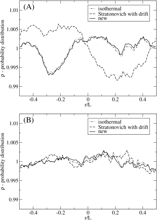
Figure 2: Probability distribution computed using the isothermal (dashed-dotted), corrected-Stratonovich (dashed), and the new convention of this paper (solid line), for (A) $dt=0.1$ and (B) $dt=0.025$. Results for the isothermal convention are replotted from Fig. 1. In the new convention, the trajectories are generated using Eqs. (LABEL:pos-equation)-(LABEL:vel-equation), with $\bar{\alpha}_{r}$ and $\bar{\alpha}_{t}$ given by Eq (4) and (6), respectively. In the corrected-Stratonovich convention, both $\bar{\alpha}_{r}$ and $\bar{\alpha}_{t}$ are given by Eq (4), and the newly computed position, $r^{n+1}$, is shifted by $-[\alpha^{\prime}(r^{n})/\alpha(r^{n})](k_{B}T/m)(dt^{2}/4)$ to correct for the spurious drift.

III The Drift

We have argued above that the noise-term in Eq. (3) should have zero mean when averaged over all possible noise realizations during one time step. To satisfy the second law of thermodynamics, the friction term in Eq. (3) must also have a zero mean; yet, this is not true for each time step, but rather upon averaging over an ensemble of Brownian particles that leave from $r^{n}$ with the Maxwell-Boltzmann velocity distribution (or, equivalently, upon averaging over all the occasions that a single particle travels through at $r^{n}$ in the long time limit). This requirement is necessary to ensure that the statistical-mechanical average change in the momentum of the particle vanishes and, therefore, that no real force acts on the particle while it diffuses in a flat potential. Thus, $\langle\bar{\alpha}_{r}\Delta r\rangle=0$, where $\Delta r=r^{n+1}-r^{n}$ ensures that no average momentum is contributed to the particle by the noise. Using the approximation $\bar{\alpha}_{r}\simeq\alpha(r^{n})+\alpha^{\prime}(r^{n})\Delta r/2$, this condition leads to

$$\alpha(r^{n})\langle\Delta r\rangle\simeq-\frac{\alpha^{\prime}(r^{n})}{2}\left\langle(\Delta r)^{2}\right\rangle=-\frac{\alpha^{\prime}(r^{n})}{2}\frac{k_{B}T}{m}dt^{2},$$ (9)

where the second equality is obtained by virtue of the equilibrium Maxwell-Boltzmann velocity distribution, and the fact that to linear order in $dt$, $\Delta r\simeq v^{n}dt$ and, therefore, $\langle(\Delta r)^{2}\rangle\simeq\langle(v^{n})^{2}\rangle dt^{2}=(k_{B}T/m)dt^{2}$. From Eq. (9) we conclude that the particle’s mean drift is given by

$$\langle\Delta r\rangle=-\frac{1}{2}\frac{\alpha^{\prime}(r^{n})}{\alpha(r^{n})}\frac{k_{B}T}{m}dt^{2}.$$ (10)

The associated force $f_{s}=-k_{B}T\alpha^{\prime}/\alpha$, is the force that produces the same mean drift in a uniform medium, in which case $\langle\Delta r\rangle=(f/2m)dt^{2}$. This force is obviously not real, which is why it is denoted “spurious” footnote2 . Our derivation demonstrates that the drift originates from the dissipation, not the fluctuation, term in Langevin equation of motion. This observation is directly related to the notion that the drift represents an inertial effect arising from the feature that when the particle travels toward a less viscous regime, it experiences less friction and therefore travels longer distances. This physical picture cannot be captured within the framework of overdamped Brownian dynamics in which the inertial degree of freedom is missing. Furthermore, our derivation suggests that another term frequently used in the literature; namely “noise induced drift” is somewhat misleading. This term stems from the proportionality of the drift to $k_{B}T$. However, as our deviation demonstrates, the noise term does not produce the drift. Instead, the linearity of $\langle\Delta r\rangle$ with temperature is due to mean squared velocity (which, per se, is obviously of thermal origin). At higher temperatures, the particle moves faster and this amplifies the magnitude of the inertial effect that produces the drift.

IV Concluding Remarks

We conclude by explaining why the seemingly more physical Stratonovich interpretation fails to produce the correct equilibrium distribution, and why the isothermal convention succeeds. We first note that by multiplying Eq. (II) by $\sigma^{n+1}$, and by using the leading order approximations $\bar{\alpha}\simeq\alpha(r^{n})$ (this is true in any convention as long as $\alpha(r)$ is sufficiently smooth), $b\simeq 1$, and the relations $\langle v^{n}\sigma^{n+1}\rangle=0$, $\langle\sigma^{n+1}\rangle=0$, and $\langle(\sigma^{n+1})^{2}\rangle=1$, we find that

$$\langle\sigma^{n+1}\Delta r\rangle\simeq\sqrt{2\alpha k_{B}Tdt}\,(dt/2m),$$ (11)

where $\alpha=\alpha(r^{n})$ for brevity. Now, as shown above, the the drift given by Eq. (10) originates from the dissipation term in Eq. (3), while the noise term in that equation has a zero mean. The Stratonovich convention interprets the friction term in essentially the same manner as our convention, but it also incorrectly assumes that $\bar{\alpha}_{t}=\bar{\alpha}_{r}$. While this seems like a minor difference, it directly causes the noise term to produce undesirable drift. Specifically, in the Stratonovich picture the noise term in Eq. (3) is given by $\sqrt{2\bar{\alpha}_{r}k_{B}Tdt}\sigma^{n+1}$, the mean value of which should be added to the middle part of Eq. (9). Using the expansion $\bar{\alpha}_{r}\simeq\alpha+\alpha^{\prime}\Delta r/2$ and the relationship expressed by Eq. (11), we find that the noise term in the Stratonovich convention generates a drift of size $\langle\Delta r\rangle=+(\alpha^{\prime}/\alpha)(k_{B}T/m)(dt^{2}/4)$, which eliminates half of the drift from the dissipation term. This error in the Stratonovich convention can be corrected by simply shifting the value of $r^{n+1}$ computed by the Langevin integrator Eqs. (LABEL:pos-equation)-(LABEL:vel-equation) by $-(\alpha^{\prime}/\alpha)(k_{B}T/m)(dt^{2}/4)$. The corrected-Stratonovich convention (which, as demonstrated in Fig. 2, also produces a fairly uniform distribution) corresponds to the overdamped limit of the Langevin equation when reached by adiabatic elimination of the velocity sancho . In the isothermal convention, $\alpha(r^{n+1})\simeq\alpha+\alpha^{\prime}\Delta r$ is used in both the dissipation and noise terms. When compared to the Stratonovich case, the difference is that $\alpha(r^{n+1})-\alpha(r^{n})\simeq 2[\bar{\alpha}_{r}-\alpha(r^{n})]$. This implies that in the isothermal convention, the dissipation term produces a drift which is twice larger than necessary, and the noise term eliminates half of this drift to bring it to just the right value. In other words, the isothermal convention benefits from the cancellation of two errors. The new convention, presented here, produces the correct drift from the dissipation term, and no drift (as should be) from the noise. We argue that this feature makes it the most physical approach, despite of the fact that all the three methods presented in Fig. 2 produce distributions that closely match the uniform equilibrium distribution.

- (1) W. T Coffey, Y. P. Kalmyfov, and J. T. Waldron, The Langevin equation: With application in physics, chemistry and electrical engineering (World Scientific, London, 1996).
- (2) G. Parisi,Statistical field theory (Addison Wesley, Menlo Park, 1988).
- (3) N. G. van Kampen, Stochastic processes in physics and chemistry (North-Holland, Amsterdam, 1981).
- (4) R. Kubo, Rep. Prog. Phys. 29, 255 (1966).
- (5) J. L Doob, Ann. Math 43, 351 (1942).
- (6) R. Mannella and V. P. E McClintock, Fluct. Noise Lett. 11 1240010 (2012).
- (7) K. Itô, Proc. Imp. Acad. Tokyo 20, 519 (1944).
- (8) R. L. Stratonovich, SIAM J. Contol. 4, 362 (1966).
- (9) P. Hänggi, Helv. Phys. Acta 51, 183 (1978).
- (10) A. W. C. Lau and T. C. Lubensky, Phys. Rev. E 76, 011123 (2007).
- (11) Strictly speaking, the “end of the time step” convention may not produce the correct equilibrium statistics in dimensions higher than 1, see discussion in M. Hütter and H. C. Öttinger, J. Chem. Soc., Faraday Trans. 94, 1403 (1998).
- (12) G. Volpe, L. Helden, T. Brettschneider, J. Wehr, and C. Bechinger, Phys. Rev. Lett. 104, 170602 (2010).
- (13) J. M. Sancho, Phys. Rev. E 84, 062102 (2011).
- (14) P. F. Tupper and X. Yang, Proc. R. Soc. A 468, 3864 (2012).
- (15) R. Kupferman, G. A Pavliotis, and A. M. Stuart, Phys. Rev. E. 70, 036120 (2004).
- (16) H. Risken, The Focker-Planck equation (Springer-Verlag, Berlin, 1988).
- (17) N. Grønbech-Jensen and O. Farago, Mol. Phys. 111, 983 (2013).
- (18) D. T. Gillespie, Markov processes: An introduction for physical scientists (Academic, San Diego, 1992).
- (19) The spurious force cannot be introduced into the Langevin equation as a real force since, unlike real forces, it cannot be associated with a potential energy gradient that leads to variations in the equilibrium distribution.