The Bolocam Galactic Plane Survey IX: Data Release 2 and Outer Galaxy Extension

Abstract

We present a re-reduction and expansion of the Bolocam Galactic Plane Survey, first presented by Aguirre et al. (2011a) and Rosolowsky et al. (2010a). The BGPS is a 1.1 mm survey of dust emission in the Northern galactic plane, covering longitudes $-10^{\circ}<\ell<90^{\circ}$ and latitudes $|b|<0.5^{\circ}$ with a typical $1-\sigma$ RMS sensitivity of 30-100 mJy in a $\sim 33\mbox{${}^{\prime\prime}$}$ beam. Version 2 of the survey includes an additional $\sim 20$ square degrees of coverage in the 3rd and 4th quadrants and $\sim 2$ square degrees in the 1st quadrant. The new data release has improved angular recovery, with complete recovery out to $\sim 80\mbox{${}^{\prime\prime}$}$ and partial recovery to $\sim 300\mbox{${}^{\prime\prime}$}$, and reduced negative bowls around bright sources resulting from the atmospheric subtraction process. We resolve the factor of 1.5 flux calibration offset between the v1.0 data release and other data sets and determine that there is no offset between v2.0 and other data sets. The v2.0 pointing accuracy is tested against other surveys and demonstrated to be accurate and an improvement over v1.0. We present simulations and tests of the pipeline and its properties, including measurements of the pipeline’s angular transfer function.

The Bolocat cataloging tool was used to extract a new catalog, which includes 8594 sources, with 591 in the expanded regions. We have demonstrated that the Bolocat 40^′′ and 80^′′ apertures are accurate even in the presence of strong extended background emission. The number of sources is lower than in v1.0, but the amount of flux and area included in identified sources is larger.

1 Introduction

Observations in the millimeter continuum provide the best method to identify a Galaxy-wide sample of star-forming clumps. The emission is optically thin, minimally affected by temperature and can be surveyed over large areas. Unlike targeted observations, blind surveys allow for a complete and systematic study of dense gas clumps.

In the past decade, there have been many Galactic plane surveys at millimeter/submillimeter wavelengths, of which the Bolocam Galactic Plane Survey (Aguirre et al. 2011a; Rosolowsky et al. 2010b) was the first to be completed and publicly released. ATLASGAL (Schuller et al. 2009) surveyed the southern Galactic plane at 870 $\mu\textrm{m}$. The JCMT Galactic Plane Survey, or JPS, will survey the Northern plane at 850 $\mu\textrm{m}$. In the past 3 years, the Hi-Gal Galactic Plane survey observed the Galaxy from 70 to 500 $\mu\textrm{m}$ with the Herschel Space Observatory, sensing the peak of the dust SED with minimal spatial filtering (Molinari et al. 2010a). The survey has provided access to the peak of the dust spectral energy distribution at modest ($\lesssim 40\mbox{${}^{\prime\prime}$}$) resolution (Traficante et al. 2011). Together, these surveys provide a complete map of long-wavelength dust emission across the Galactic plane.

Long-wavelength data are essential for constraining the dust emissivity, one of the free parameters in greybody spectral energy distribution (SED) fits. Shetty et al. (2009a, b) demonstrated the need for long-wavelength data to accurately determine both $\beta$, the dust emissivity spectral index, and temperature. Juvela & Ysard (2012) also showed that adding additional wavelengths to an SED fit, even with lower signal-to-noise, significantly reduces the degeneracy in the fit.

Millimeter-wave dust emission also has the advantage of being relatively insensitive to temperature. When looking at cold gas, $T\lesssim 20$ K, all of the Herschel bands deviate from a Rayleigh-Jeans temperature approximation. Longer wavelength observations are less affected by temperature assumptions. The 1.1 mm band is in many cases the longest wavelength unaffected by free-free emission, providing the least environmentally-biased view of optically thin dust emission and therefore total dust mass.

Similarly, at millimeter wavelengths, the dust opacity is low enough that all clumps detected in the BGPS are expected to be optically thin (with the possible exception of Sgr B2; Bally et al. 2010). In combination with the weak temperature dependence, this feature of 1.1 millimeter emission allows for the most direct and straightforward estimates of total dust mass.

Millimeter-bright dust clumps are generally associated with high-density, star-forming gas. Previous surveys have found cold, massive molecular clouds via the ${}^{12}\textrm{CO}$ and ${}^{13}\textrm{CO}$ 1-0 lines (Dame et al. 2001a; Jackson et al. 2006). However, these clouds are only moderate density, $n(\textrm{H}_{2})\sim 10^{2}-10^{3}$ $\textrm{cm}^{-3}$, while dust-detected clumps have typical densities $n(\textrm{H}_{2})\gtrsim 10^{4}$ $\textrm{cm}^{-3}$(Dunham et al. 2010). The dense gas in these clumps is more directly associated with star and cluster formation (Dunham et al. 2011a; Battersby et al. 2010), allowing for systematic studies of pre-star-forming and star-forming gas.

The BGPS v1.0 data has been public since 2009, and has been used extensively as both a finder chart and a tool to probe Galactic properites. It was used to examine the properties of maser sources (Pandian et al. 2012; Chen et al. 2012), outflow sources (Ioannidis & Froebrich 2012), and high-mass star-forming regions (Reiter et al. 2011; Battersby et al. 2011; Dunham et al. 2011b). It has served as the basis for studies of forming clusters (Alexander & Kobulnicky 2012; Ginsburg et al. 2012) and intermediate-mass stars (Arvidsson et al. 2010). The BGPS and other surveys have served as finder charts for large-scale millimeter line studies of the Galactic plane (Schenck et al. 2011; Schlingman et al. 2011; Ginsburg et al. 2011; Shirley et al. 2013). BGPS clumps have been used as the target sample for distance determinations to large cloud populations (Ellsworth-Bowers et al. 2013). Dunham et al. (2011a) used the BGPS to measure properties of star forming regions as a function of Galactocentric radius. These and many other ongoing and planned studies demonstrate the need for, and benefits of, publicly available blind legacy surveys.

This paper presents v2.0 of the Bolocam Galactic Plane Survey (BGPS), with a complete data release available at irsa.ipac.caltech.edu/data/BOLOCAM_GPS/. In Paper I (Aguirre et al. 2011a), the initial processing of the BGPS v1.0 was described in detail. It was noted in Section 5 of Aguirre et al. (2011a) that there was a discrepancy between our survey and previously published results. This discrepancy raised the possibility of a flux calibration error in the Version 1 (hereafter v1.0) results: we confirm and correct the error in this paper. In addition, we have made significant improvements to the data pipeline, measured important features of the pipeline including its angular transfer function, improved the pointing accuracy, and added new observations.

The paper is as follows: We resolve the flux calibration discrepancy in Section 2. In Section 3, we discuss new observations included in the v2.0 data. Section 4 describes changes to the data reduction process and new data products. Section 5 and Section 6 measure the angular transfer function of the BGPS v2.0 pipeline and properties of extracted sources respectively. The paper concludes with a brief discussion of the results and a summary.

2 Calibration

The original calibration, along with tables of color correction and a detailed treatment of the filter response, are described in Aguirre et al. (2011b). We discuss important changes in v2.0 in this section.

2.1 Why was there a multiplicative offset in the v1.0 data release?

In Aguirre et al. (2011a), we reported that a ‘correction factor’ of about 1.5 on average was needed to bring our data into agreement with other 1 mm data sets. We discovered that the published v1.0 BGPS images have a different calibration reported in their FITS headers than was used in processing the data. The calibration used in the released data was borrowed from a previous observing run, during which a different bias voltage was used, and differed from the pipeline-derived calibration by a factor $\approx 1.5$, completely explaining the discrepancy.

2.2 Comparing v1.0 and v2.0 calibration

We checked the data for consistency with the measured calibration offset. In order to compare flux densities in identical sources, we performed aperture photometry on the v2.0 data based on the locations of v1.0 sources using both the ‘source masks’ from Bolocat v1.0 (Rosolowsky et al. 2010a) and circular apertures centered on the Bolocat v1.0 peaks. Source masks, also known as label masks, are images in which the value of a pixel is either 0 for no source or the catalog number if there is a source associated with that pixel.

We measured the multiplicative offset between v1.0 and v2.0 by comparing these aperture-extracted fluxes. For each aperture size, we measured the best-fit line between the v1.0 and v2.0 data using a total least squares (TLS) method weighted by the flux measurement errors as reported in the catalogs. The agreement with $S_{{\rm v}2.0}=1.5~{}S_{{\rm v}1.0}$, as expected based on Section 2.1, is within 10%, although the larger apertures show a slight excess with $S_{{\rm v}2.0}\approx(1.6\mathchar 45\relax 1.7)~{}S_{{\rm v}1.0}$. This excess is expected given the improved extended flux recovery in v2.0 (see Section 5). The v2.0/v1.0 flux ratio is weakly dependent on the source flux density, with higher v2.0/v1.0 ratios for brighter sources.

2.3 Comparison to Other Surveys

In Section 5.5 of Aguirre et al. (2011a), we compared the BGPS v1.0 data to other data sets from similar-wavelength observations. We repeat those comparisons here using the v2.0 data and demonstrate that v2.0 achieves better agreement with other data sets than v1.0. Full details of the comparison were given in Aguirre et al. (2011b).

We compare to 3 data sets in the same $\sim 1$ mm atmospheric window. Two data sets from MAMBO II, the Motte et al. (2007, M07) Cygnus X survey and the Rathborne et al. (2006, R06) IRDC survey, overlap with the BGPS. The SIMBA 1.3 mm survey of the $\ell=44^{\circ}$ region is the largest survey in the 1 mm band that overlaps with ours (Matthews et al. 2009, M09).

The comparison data sets have angular transfer functions that differ from the BGPS. In order to account for the difference, we allow for a large angular scale offset between the observations. We fit a line of the form $y=mx+b$ to the data, where $x$ and $y$ represent the pixel values gridded to 7.2^′′ pixels. The $b$ value allows for a local offset, i.e. a non-zero $b$ value indicates a substantial difference in the angular transfer function. Since such an additive offset is unlikely to apply across the entire observed region, we also fit the offset for small sub-regions in the M07 and M09 data, focusing on DR21 and a region centered on G45.5+0.1 respectively.

Table 1: Flux comparison with R06, M07, and M09

Comparison	Pixels		Pixels		Pixels
Survey	$>3~{}{\rm MJy~{}sr}^{-1}$		$>10~{}{\rm MJy~{}sr}^{-1}$		$>20~{}{\rm MJy~{}sr}^{-1}$
BGPS v1.0	$m$	$b$	$m$	$b$	$m$	$b$
R06	1.39	$-2.00$	1.46	$-2.79$	1.53	$-4.77$
M07	1.51	$4.13$	1.44	$13.78$	1.36	$27.45$
M07DR21	1.36	$28.03$	1.31	$37.91$	1.25	$49.44$
M09	1.32	$-0.22$	1.25	$4.94$	1.21	$9.88$
M09a	1.50	$-5.15$	1.51	$-4.82$	1.53	$-5.11$
BGPS v2
R06	1.05	$3.67$	1.02	$5.03$	1.00	7.05
M07	1.16	$6.51$	1.12	$12.75$	1.08	21.04
M07DR21	1.09	$21.98$	1.07	$27.61$	1.04	34.21
M09	0.73	$1.33$	0.69	$6.75$	0.66	13.45
M09a	0.96	$-3.21$	0.94	$-0.69$	0.89	2.91

The table values $m$ and $b$ are given for a linear fit of the form $y=mx+b$.
References: Rathborne et al. (2006, R06; MAMBO), Motte et al. (2007, M07; MAMBO), Matthews et al. (2009, M09; SIMBA).
M09a refers to the G45.5+0.1 region, and M07DR21 refers to the DR21 region

The results of that comparison are displayed in Table 1, which includes the original comparison from Aguirre et al. (2011a). BGPS v2.0 is in much better agreement with the other data sets than v1.0, but it retains a significant additive offset, particularly with respect to MAMBO. The additive offset is explained by a difference in the angular transfer function; the MAMBO observing strategy of fast position switching allows structures on the scale of the array to be preserved, while Bolocam’s fast-scan strategy does not. The differing observing strategy explains why there is an additive offset between Bolocam and MAMBO, but no such offset for SIMBA, which was used in a fast-scan mode similar to Bolocam. The varying backgrounds in separate regions account for some of the remaining multiplicative offset. When individual sub-regions are compared, the additive and multiplicative offsets more clearly separate into independent components, i.e. a line with an additive offset is a better fit to the data.

To enable a comparison of flux density between the surveys, we must account for the different spectral bandpasses of the instruments. The relative flux density measured between the instruments depends on the spectral index $\alpha_{\nu}$ of the observed source; $\alpha_{\nu}=2$ corresponds to a perfect black body on the Rayleigh-Jeans tail. In Table 2 we show the relative flux densities expected for Bolocam, MAMBO and SIMBA; they differ by at most 19% for spectral indices $\alpha_{\nu}<5$. Bolocam flux densities are expected to be higher because Bolocam has a higher effective central frequency than either of the other instruments.

In Aguirre et al. (2011a), we measured Bolocam v1.0/MAMBO and Bolocam v1.0/SIMBA ratios in the range $0.66<R<0.83$, indicating a clear disagreement between the surveys. With the v2.0  data, we measure ratios $0.97<R_{SIMBA}<1.08$ and $0.89<R_{MAMBO}<0.99$. These numbers still indicate that the BGPS is too faint by $\lesssim 20\%$ relative to the expectations laid out in Table 2, but with a systematic calibration error no better than 20% in each survey, this level of agreement is reasonable.

Table 2: Relative flux measurements of Bolocam, MAMBO, and SIMBA for different input sources

$\alpha$	Bolocam/MAMBO	Bolocam/SIMBA
1.0	1.092	1.096
1.5	1.092	1.096
2.0	1.092	1.096
2.5	1.110	1.119
3.0	1.126	1.140
3.5	1.138	1.157
4.0	1.146	1.170
4.5	1.151	1.181
5.0	1.152	1.188

Response functions are computed using an atmospheric transmittance of 1 mm of precipitable water vapor.

3 Expansion of the BGPS and Observations

Thirteen nights of additional data were acquired from December 15th, 2009 to January 1st, 2010. The target fields and areas covered are listed in Table 3 as boxes in Galactic latitude and longitude, with position angles to the Galactic plane indicated. The original observations are described in Section 2 of Aguirre et al. (2011a).

Table 3: Observations

Target	Longitude	Latitude	Longitude Size	Latitude Size	Position Angle
IRAS 22172	102.91	-0.64	1.67	1.07	0
l106	105.81	0.15	1.48	1.33	0
l111w	108.23	-0.43	3.35	2.78	0
l111n	110.50	2.18	4.19	2.21	0
l111s	111.07	-1.64	2.32	1.10	0
l119	119.40	3.08	3.29	0.83	330
l123	123.68	2.65	2.87	1.07	12
l126	125.70	1.93	1.06	1.08	0
l129	129.21	0.11	1.82	1.63	0
camob1	141.20	-0.31	2.79	3.40	0
l154	154.83	2.38	1.68	1.27	0
l169	169.42	-0.32	4.08	2.05	0
sh235	172.94	2.50	4.60	1.34	0
l181	181.11	4.40	2.19	1.20	0
l182	182.36	0.23	3.25	1.18	28
l195	195.92	-0.66	3.04	1.18	56
l201	201.57	0.30	1.32	1.37	0
ngc2264	202.97	2.21	2.20	1.32	0
orionBnorth	204.01	-11.86	2.17	1.33	335
orionB	206.73	-16.21	2.36	2.35	30
orionAspine	212.45	-19.24	4.35	2.48	0
monr2	213.54	-12.13	2.70	2.78	0
l217	217.69	-0.24	1.91	1.04	0

All numbers are in degrees.

The new target fields were selected from visual inspection of FCRAO OGS ${}^{12}\textrm{CO}$ integrated maps, Dame et al. (2001b) ${}^{12}\textrm{CO}$ maps, and IRAS 100 $\mu\textrm{m}$  maps. The fields were selected primarily to provide even spacing in RA in order to maximize observing efficiency, and were therefore not blindly selected.

Additionally, the Orion A and B and Mon R2 clouds were observed in observing campaigns by collaborators. These complexes are not directly part of the BGPS, but are included in this data release reduced in the same manner as the Galactic plane data. They are much closer than typical BGPS sources and their selection for mapping is very biased, but we include them in the archival data. Parts of the Orion A nebula remain proprietary as of this release, but are expected to be released upon publication of Kauffmann et al (in prep). The California nebula has also been observed and the data published in Harvey et al. (2013).

Finally, some archival CSO data was recovered and added to the BGPS. These data include maps of M16 and M17. M17 is an extraordinarily bright 1.1 mm source that was poorly covered in the BGPS because it is below $b=-0.5$.

The Bolocat cataloging tool was run on these new fields and they have been included in the v2.0 catalog. Some of their properties are displayed in Section 6. A total of 591 new sources not covered in the v1.0 survey were extracted.

4 Data Reduction and Data Products

4.1 A brief review of ground-based millimeter observational techniques

Observations at wavelengths longer than 2 $\mu\textrm{m}$ and shorter than 2 cm from the ground are strongly affected by emission and absorption from our own atmosphere. Optical and radio observations from the ground see through a transparent atmosphere, but millimeter observations are dominated by bright foreground emission that dominates the astrophysical signal. This foreground must be removed in order to create maps of astrophysical emission.

Chapin et al. (2013) presented a summary of the techniques used to separate astrophysical and atmospheric signals in (sub)millimeter bolometric observations. The Bolocam observations reported in this paper were conducted with a fast-scanning strategy that places some of the ‘fixed’ astrophysical emission at a different sampling frequency than the varying foreground atmosphere. This approach is one of the most efficient and flexible and has been used predominantly over alternatives, such as a nodding secondary, in most recent large-scale observing campaigns (Aguirre et al. 2011a; Schuller 2012).

A variety of different atmospheric removal algorithms have been successfully utilized, but in addition to removing the atmospheric foreground, these approaches remove some of the astrophysical signal. In order to recover signal on angular scales up to the array size, the most commonly used approach for bright Galactic signals is an iterative reconstruction process. This process assembles a model of the astrophysical emission, subtracts it from the observed timestream, and repeats, each time reducing the amount of astrophysical signal that is removed by the algorithm. This general approach was first used on Bolocam data by Enoch et al. (2006) and refined in Aguirre et al. (2011a). We directly examine the effects of the data reduction methods below.

4.2 Sky Subtraction

We compared a few different methods for atmospheric subtraction and astrophysical image reconstruction, but settled on an approach very similar to that used in v1.0. This subsection recounts the minor changes from v1.0 and includes discussion of alternative approaches.

The PCA method (Enoch et al. 2006, 2007) with iterative flux density restoration was used for v2.0 as for v1.0. In the PCA atmosphere removal method, the $n$ eigenvectors corresponding to the highest values along the diagonal of the covariance matrix (the most correlated components) are nulled. We nulled 13 PCA components in both v1.0 and v2.0. The selection of 13 components produced the best compromise between uniform background noise and fully restored peak signal. Simulations show that the point source recovery is a very weak function of number of PCA components nulled (nPCA), while extended flux recovery is a strong function of nPCA. However, residual atmospheric signal was substantially reduced with higher nPCA. In v2.0, 20 iterations were used instead of the 50 used in v1.0; in both surveys, convergence was clearly achieved by 20 iterations, and generally individual iterations are indistinguishable by $\sim 5$ iterations.

The iterative process adopts the non-negative flux density above some cutoff as a model of the astrophysical sky and subtracts that flux density from the timestream before repeating the atmospheric subtraction. This approach allows large angular scale structures to be recovered by removing them from the timestreams before they can contribute to the correlated signal.

The v2.0 pipeline was more succesful than in v1.0 at removing negative bowls (see Section 6.2 for visual examples). Negative bowls are introduced because the atmospheric subtraction process assumes that the mean level of any timestream, and therefore any map, is zero. The iterative process allows this assumption to be violated, creating maps with net positive signal.

The reduced impact of negative bowls is attributed to a few small changes to the pipeline that each slightly mitigate the bowls.

1. The astrophysical model is created by deconvolving the positive emission rather using positive pixels directly. The deconvolution process, which removes sub-beam-scale noise, was made more stable in v2.0 by performing a local signal-to-noise cut using the noise maps described in Section 4.3.1; in v1.0 there was no reliable noise map available during the iterative map making process.

2. Better image co-alignment reduced inter-observation spatial offsets. The astrophysical models therefore better reproduced the timestream data.

3. Improvement in the bolometer gain calibration, which is done on a per-observation basis in v2.0, improved the convergence of the iterative map maker.

These changes are individually minor, but together resulted in significant improvements to the map quality.

The quadratic planar fit sky subtraction method discussed in Sayers et al. (2010) was implemented and tested for 1.1mm Galactic plane data in the v2.0 pipeline, but was not used for the final data products. In principle, this method should do a substantially better job at removing smooth atmospheric signal from timestreams than PCA cleaning because it is based on physically expected atmospheric variation. The spatial recovery was better than the aggressive 13-PCA approach, but as with a simpler median subtraction approach (subtracting the median timestream from all bolometers), a great deal of spurious signal from the atmosphere remained in the maps, and the noise properties were highly non-uniform, rendering source extraction difficult. It was also more computationally expensive and did not remove correlated electronic readout noise, which PCA subtraction did. The Sayers et al. (2010) approach is likely more effective at 143 GHz because the atmosphere is better-behaved at lower frequencies. We speculate that it is also more effective for deep extragalactic fields in which more repeat observations of the same field are able to distinguish atmospheric from real signal on the angular scales of the array.

4.3 Data products

The BGPS data are available from the Infrared Processing and Analysis Center (IPAC) at irsa.ipac.caltech.edu/data/BOLOCAM_GPS/. The v2.0 data products include the pipeline-processed maps and Bolocat label masks as in v1.0.

In the v2.0 data release, there are two new map types released: noise maps and median maps. A variant of the noise maps was produced in v1.0, while the median maps are an entirely new data product.

4.3.1 Noise Maps

Residual bolometer timestreams are automatically generated as part of the iterative map-making process. The residual is the result of subtracting the astrophysical model (which is smooth, noiseless, and non-negative) from the atmosphere-subtracted data timestream. The resulting timestream should only contain the remaining astrophysical noise. However, maps of the residual timestream contain sharp edge features because the astrophysical model is sharp-edged (i.e., transitions from 0 to a non-zero value from one pixel to the next). These sharp transitions are mitigated in the presence of noise.

We therefore created noise maps by taking the local standard deviation of the residual map. Pixels in the original map that were not sampled (i.e., represented by NaN in the FITS data file) are ignored when computing this local standard deviation and their values are set to be an arbitrarily high number ($100$ Jy/beam) such that pixels near the map edge are assumed to have extremely high noise (which is reasonable, since these pixels are affected by a variety of artifacts rendering them unreliable measurements of the true astrophysical flux). The local noise is computed within a $FWHM=10$-pixel gaussian, which enforces a high noise level within $\sim 2\mbox{${}^{\prime}$}$ of the map edge. This method produces good noise maps (i.e., in agreement with the standard deviation calculated from blank regions of the signal map) and was used both within the iterative process and for cataloging.

We show the noise per pixel for each half square degree in the inner galaxy in Figure 1. The noise level in each outer-galaxy field is summarized in Figure 2. Because the outer galaxy coverage is irregular, we show the noise per observed region rather than dividing the regions into degree-scale sub-regions.

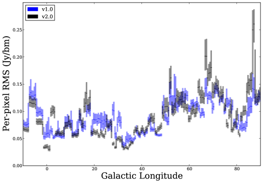
Figure 1: Map noise for 0.5 degree cuts in longitude in the range $|b|<0.5^{\circ}$. The solid horizontal lines show the median noise in the map, while the shaded regions highlight the 1-$\sigma$ (68%) interval (quantiles 16-84) of the noise. The noise is the local weighted standard deviation (rms) over a $FWHM=10$-pixel region (see Section 4.3.1).

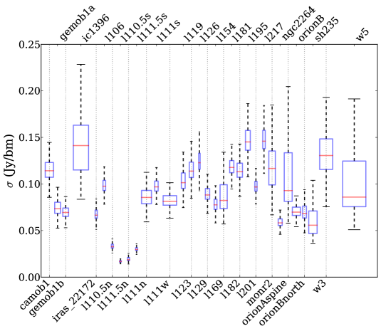
Figure 2: The noise in each outer galaxy field shown with box plots. The red lines indicate the median, the boxes show the 25%-75% range, and the black dashed lines (‘whiskers’) show the 16%-84% (1-$\sigma$) range. Unlike Figure 1, the field size for each region varies, which is why there is a much broader spread in the widths of the individual noise distributions. The size of the region is proportional to the box width.

4.4 Median Maps

Some artifacts (cosmic ray hits, instrumental artifacts) inevitably remained at the end of the process. In order to mitigate these effects, “median maps” were created. The value of each spatial pixel was set to the median value of the timestream points intersecting that pixel; pixels with fewer than 3 data points were set to NaN. The noise in the median maps was in some cases lower than that in the weighted mean maps, particularly for fields with fewer total observations. They uniformly have mitigated instrument-related artifacts such as streaking. These maps are released in addition to the weighted-mean maps, which often have higher signal-to-noise.

4.5 Pointing

In order to get the best possible pointing accuracy in each field, all observations of a given area were median-combined using the montage package, which performs image reprojections, to create a pointing master map (Berriman et al. 2004). Each individual observation was then aligned to the master using a cross-correlation technique (Welsch et al. 2004):

1. The master and target image were projected to the same pixel space

2. A cross-correlation image was generated, and the peak pixel in the cross-correlation map was identified

3. Sub-pixel alignment was measured by performing a 2nd-order Taylor expansion around the peak pixel

This method is similar to the version 1.0 method, but the new peak-finding method proved more robust than the previous Gaussian fitting approach. The v1.0 Gaussian fitting approach is often used in astronomy (e.g., http://www.astro.ucla.edu/~mperrin/IDL/sources/subreg.pro), but it is biased when images are dominated by extended structure. This bias occurs because the least-squares fitting approach will identify the broader peak that represents auto-correlation of astrophysical structure rather than the cross-correlation between the two images. In v1.0, we attempted to mitigate this issue by subtracting off a ‘background’ component before fitting the Gaussian peak, but this method was not robust.

The improved approach to pointing resulted in typical RMS offsets between the individual frames and the master $\sigma_{\mathbf{x}}\sim 2$ ^′′. The improvement in the point spread function is readily observed (see Section 6.2).

4.6 Pointing Comparison

We carefully re-examined the pointing throughout the BGPS using a degree-by-degree cross-correlation analysis between the v1.0, v2.0, and Herschel Hi-Gal 350 $\mu\textrm{m}$ data. The Herschel data were unsharp-masked (high-pass filtered) by subtracting a version of the data smoothed with a $\sigma=120\mbox{${}^{\prime\prime}$}$ Gaussian. The result was then convolved with a $\sigma=8.9\mbox{${}^{\prime\prime}$}$ Gaussian to match the Herschel to the Bolocam beam sizes.

Errors on the offsets were measured utilizing the Fourier scaling theorem to achieve sub-pixel resolution (inspired by Guizar-Sicairos & Fienup 2008). The errors on the best-fit shift were determined using errors estimated from the BGPS data and treating the filtered Hi-Gal data as an ideal (noiseless) model. The tools for this process, along with a test suite demonstrating their applicability to extended structures in images, are publicly available at http://image-registration.readthedocs.org/.

The cross-correlation technique calculated the $\chi^{2}$ statistic as a function of the offset. For a reference image $Y$ and observed image $X$ with error per pixel $\sigma_{xy}$,

$$\chi^{2}=\sum\frac{(X-Y(\Delta x,\Delta y))^{2}}{\sigma_{xy}^{2}}$$

where $\Delta x$ and $\Delta y$ are the pixel shifts. Because Y is not actually an ideal model but instead is a noisy image, we increase $\sigma_{xy}$ by the rms of the difference between the aligned images, using a corrected $\sigma_{c}^{2}=\sigma_{BGPS}^{2}+RMS(X-Y(\Delta x_{b},\Delta y_{b}))$, where $\Delta x_{b},\Delta y_{b}$ are the best-fit shifts.

For the majority of the examined 1-square-degree fields, the signal dominated the noise and we were able to measure the offsets to sub-pixel accuracy. A plot of the longitude / latitude offsets between v2.0 and v1.0 and Herschel Hi-Gal is shown in Figure 3.

Table 4 lists the measured offsets in arcseconds between images for all 1 degree fields from $\ell=351\mbox{${}^{\circ}$}$ to $\ell=65\mbox{${}^{\circ}$}$. The offsets represent the Galactic longitude and latitude shifts in arcseconds from the reference (left) to the ‘measured’ field (right).

Table 5 shows the means of the columns in Table 4, weighted by the error in the measurements and by the number of sources. Weighting by the number of sources is used for comparison with other works that attempt to measure the pointing offset on the basis of catalog source position offsets. None of the measured offsets are significant; in all cases the scatter exceeds the measured offset.

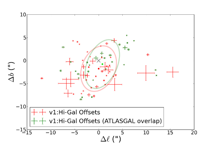
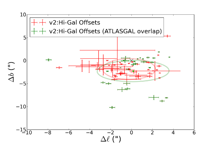
Figure 3: Plots of the latitude and longitude offsets of individual 1-degree fields in v1.0 (a) and v2.0 (b) as compared with Herschel Hi-Gal. Offsets were measured using a cross-correlation technique described in the text. The error bars correspond to $\Delta\chi^{2}<2.3$, or $1-\sigma$ for Gaussian distributed noise and 2 degrees of freedom. The circles and ellipses represent the mean and standard deviation (unweighted) offsets in the whole survey (red) and the $(351\mbox{${}^{\circ}$}<\ell)\cup(\ell<20\mbox{${}^{\circ}$})$ ATLASGAL-overlap regions (green). In both cases, the mean offset is consistent with zero (shown as a black x), but many individual fields show significant offsets. Note that the scales are different; there are far fewer outliers in the v2.0-Herschel comparison (b) and the average offset is much closer to zero. The errors are larger in the non-ATLASGAL overlap region because there is less signal in the $35\mbox{${}^{\circ}$}<\ell<65\mbox{${}^{\circ}$}$ range.

Table 4: Cross-Correlation Offsets

Field Name	$\Delta\ell$(HG-v2)	$\Delta b$(HG-v2)	$\Delta\ell$(v1-v2)	$\Delta b$(v1-v2)	$\Delta\ell$(HG-v1)	$\Delta b$(HG-v1)	N(v1 sources)
l351	$0.37(-0.21)$	$-0.65(0.21)$	$3.12(-0.16)$	$1.83(0.14)$	$-2.17(-0.19)$	$-2.33(0.19)$	56
l352	$1.10(-0.07)$	$0.37(0.07)$	$3.14(-0.06)$	$1.45(0.06)$	$-1.93(-0.07)$	$-0.97(0.07)$	87
l353	$3.35(-0.13)$	$-8.07(0.13)$	$-3.80(-0.08)$	$-12.41(0.08)$	$7.39(-0.12)$	$4.30(0.12)$	65
l354	$2.14(-0.48)$	$-7.98(0.50)$	$-3.71(-0.11)$	$-12.04(0.09)$	$5.51(-0.43)$	$2.81(0.44)$	52
l355	$2.92(-0.20)$	$-8.78(0.20)$	$-3.57(-0.11)$	$-12.12(0.09)$	$6.24(-0.20)$	$2.42(0.20)$	54
l356	$-0.62(-0.37)$	$-0.06(0.35)$	$-1.29(-0.22)$	$-0.96(0.17)$	$0.68(-0.34)$	$1.58(0.32)$	42
l357	$-0.56(-0.43)$	$0.56(0.41)$	$-0.06(-0.24)$	$-0.39(0.17)$	$-0.56(-0.42)$	$0.56(0.39)$	23
l358	$2.14(-0.14)$	$0.56(0.14)$	$-0.62(-0.14)$	$0.17(0.12)$	$2.78(-0.14)$	$-0.25(0.14)$	35
l359	$2.63(-0.08)$	$1.90(0.06)$	$-10.05(-0.08)$	$5.86(0.07)$	$12.10(-0.10)$	$-3.21(0.07)$	248
l000	$3.61(-0.07)$	$0.77(0.06)$	$-1.10(-0.04)$	$1.55(0.03)$	$5.30(-0.07)$	$-0.89(0.06)$	318
l001	$0.59(-0.05)$	$0.37(0.07)$	$-3.36(-0.05)$	$1.31(0.06)$	$11.92(-0.16)$	$-2.02(0.11)$	368
l002	$-0.39(-0.26)$	$-6.13(0.25)$	$1.46(-0.24)$	$2.14(0.19)$	$-1.41(-0.15)$	$-7.93(0.14)$	170
l003	$-2.73(-0.21)$	$-4.75(0.20)$	$0.62(-0.18)$	$3.54(0.17)$	$-3.46(-0.10)$	$-7.96(0.10)$	243
l004	$-1.86(-0.28)$	$-10.18(0.26)$	$-0.34(-0.23)$	$0.11(0.19)$	$-3.71(-0.21)$	$-8.44(0.19)$	70
l005	$1.18(-0.29)$	$-0.28(0.28)$	$-3.99(-0.19)$	$-3.54(0.19)$	$4.39(-0.21)$	$3.49(0.19)$	78
l006	$0.83(-0.05)$	$0.60(0.06)$	$-1.17(-0.05)$	$-1.36(0.06)$	$5.88(-0.05)$	$5.48(0.05)$	109
l007	$1.97(-0.17)$	$-0.39(0.16)$	$-4.50(-0.09)$	$-4.50(0.00)$	$6.00(-0.12)$	$3.87(0.11)$	93
l008	$1.58(-0.14)$	$0.68(0.16)$	$4.58(-0.12)$	$1.43(0.15)$	$-2.39(-0.13)$	$-0.37(0.15)$	59
l009	$1.74(-0.10)$	$-1.52(0.09)$	$6.15(-0.09)$	$1.00(0.09)$	$-4.82(-0.08)$	$-2.29(0.08)$	55
l010	$0.28(-0.08)$	$-0.17(0.08)$	$3.70(-0.08)$	$1.98(0.09)$	$-4.18(-0.08)$	$-3.78(0.07)$	77
l011	$-1.05(-0.04)$	$-1.56(0.04)$	$-0.94(-0.03)$	$-0.04(0.02)$	$-1.18(-0.07)$	$-4.22(0.08)$	122
l012	$-2.31(-0.10)$	$-2.31(0.10)$	$-3.80(-0.08)$	$-0.70(0.09)$	$1.49(-0.09)$	$-1.83(0.08)$	102
l013	$-0.75(-0.05)$	$0.07(0.05)$	$-1.49(-0.05)$	$-0.59(0.05)$	$0.66(-0.05)$	$0.86(0.06)$	198
l014	$-0.28(-0.20)$	$-1.86(0.20)$	$6.05(-0.15)$	$-1.72(0.16)$	$-5.88(-0.15)$	$-0.25(0.15)$	137
l015	$-2.19(-0.26)$	$-5.01(0.26)$	$5.79(-0.17)$	$-2.64(0.19)$	$-7.93(-0.20)$	$-2.19(0.20)$	164
l016	$-0.90(-0.45)$	$-6.30(0.45)$	$5.79(-0.26)$	$-2.31(0.28)$	$-4.28(-0.25)$	$-2.92(0.20)$	63
l017	$-0.45(-0.32)$	$-4.95(0.36)$	$-1.29(-0.22)$	$-3.88(0.26)$	$2.42(-0.26)$	$1.18(0.27)$	62
l018	$0.17(-0.23)$	$-0.84(0.21)$	$-1.07(-0.17)$	$-1.97(0.17)$	$1.24(-0.15)$	$0.56(0.14)$	55
l019	$-7.93(-0.28)$	$0.17(0.25)$	$0.89(-0.11)$	$-2.69(0.10)$	$-7.42(-0.25)$	$2.92(0.23)$	179
l020	$2.43(-0.07)$	$-2.01(0.08)$	$0.07(-0.07)$	$-2.60(0.06)$	$2.50(-0.06)$	$0.70(0.06)$	110
l021	$2.64(-0.21)$	$-1.18(0.21)$	$1.86(-0.17)$	$-1.74(0.16)$	$0.68(-0.14)$	$0.68(0.14)$	103
l022	$1.74(-0.21)$	$-2.76(0.21)$	$-0.65(-0.16)$	$0.48(0.14)$	$3.57(-0.20)$	$-3.12(0.20)$	87
l023	$2.69(-0.12)$	$-3.75(0.11)$	$-0.20(-0.09)$	$-0.31(0.08)$	$3.08(-0.10)$	$-3.42(0.10)$	213
l024	$2.70(-0.09)$	$-2.70(0.09)$	$-0.44(-0.09)$	$-0.27(0.08)$	$2.32(-0.10)$	$-2.40(0.10)$	250
l025	$1.62(-0.08)$	$-1.95(0.08)$	$0.08(-0.07)$	$1.15(0.07)$	$1.65(-0.06)$	$-3.25(0.07)$	183
l026	$1.66(-0.15)$	$-0.42(0.16)$	$0.06(-0.12)$	$0.62(0.13)$	$1.72(-0.10)$	$-1.21(0.11)$	151
l027	$1.46(-0.15)$	$-0.34(0.14)$	$-0.48(-0.12)$	$0.87(0.12)$	$2.28(-0.10)$	$-1.04(0.10)$	119
l028	$2.56(-0.07)$	$1.21(0.08)$	$6.22(-0.07)$	$8.35(0.07)$	$-3.63(-0.11)$	$-7.17(0.12)$	188
l029	$-0.96(-0.11)$	$-0.73(0.11)$	$4.58(-0.09)$	$6.38(0.09)$	$-5.27(-0.09)$	$-7.27(0.09)$	177
l030	$0.06(-0.11)$	$-0.28(0.12)$	$2.05(-0.09)$	$3.23(0.11)$	$-3.21(-0.07)$	$-6.58(0.06)$	276
l031	$-1.10(-0.06)$	$-0.42(0.05)$	$-1.69(-0.03)$	$-1.46(0.02)$	$0.44(-0.07)$	$3.19(0.07)$	354
l032	$-0.24(-0.08)$	$-0.60(0.09)$	$1.18(-0.08)$	$-2.42(0.08)$	$-2.33(-0.09)$	$1.88(0.08)$	189
l033	$2.07(-0.05)$	$-2.21(0.05)$	$6.10(-0.06)$	$-5.71(0.06)$	$-4.04(-0.06)$	$3.56(0.06)$	210
l034	$-2.32(-0.09)$	$0.04(0.08)$	$-0.46(-0.05)$	$-0.10(0.05)$	$-1.55(-0.11)$	$-5.88(0.10)$	203
l035	$-1.88(-0.12)$	$-2.05(0.12)$	$0.31(-0.11)$	$-0.59(0.10)$	$-2.08(-0.13)$	$-1.41(0.12)$	247
l036	$-1.63(-0.14)$	$-0.96(0.15)$	$0.82(-0.12)$	$3.01(0.11)$	$-2.62(-0.14)$	$-4.19(0.14)$	126
l037	$-1.07(-0.32)$	$-2.87(0.29)$	$-2.31(-0.25)$	$0.51(0.24)$	$0.73(-0.23)$	$-2.31(0.21)$	83
l038	$-1.60(-0.15)$	$-3.18(0.17)$	$-0.79(-0.12)$	$0.34(0.14)$	$-0.59(-0.11)$	$-3.40(0.12)$	69
l039	$0.62(-0.26)$	$-3.43(0.24)$	$-0.23(-0.16)$	$1.12(0.14)$	$1.10(-0.19)$	$-4.30(0.17)$	69
l040	$1.74(-0.23)$	$-3.43(0.24)$	$1.86(-0.18)$	$2.98(0.17)$	$1.38(-0.17)$	$-5.20(0.16)$	40
l041	$0.23(-0.29)$	$-2.48(0.29)$	$1.07(-0.24)$	$5.23(0.20)$	$-0.96(-0.23)$	$-7.70(0.23)$	44
l042	$-1.01(-0.48)$	$-2.81(0.45)$	$0.11(-0.26)$	$5.06(0.23)$	$-2.02(-0.34)$	$-7.42(0.29)$	36
l043	$0.08(-0.10)$	$-1.15(0.09)$	$2.07(-0.08)$	$-2.52(0.09)$	$-1.74(-0.07)$	$0.84(0.05)$	17
l044	$-1.63(-0.29)$	$-4.11(0.27)$	$4.78(-0.26)$	$-8.16(0.20)$	$-4.44(-0.17)$	$4.11(0.15)$	27
l045	$-1.52(-0.16)$	$-3.43(0.15)$	$4.42(-0.14)$	$-7.73(0.12)$	$-5.36(-0.10)$	$4.32(0.09)$	30
l046	$-0.90(-0.27)$	$-2.70(0.27)$	$-1.24(-0.26)$	$-5.29(0.21)$	$1.69(-0.25)$	$3.71(0.25)$	53
l047	$0.68(-0.85)$	$-3.38(0.63)$	$0.34(-0.38)$	$-3.71(0.27)$	$3.26(-0.56)$	$4.39(0.41)$	11
l048	$-0.45(-1.35)$	$-4.05(1.31)$	$8.16(-0.27)$	$-3.32(0.30)$	$-6.08(-0.76)$	$-0.23(0.76)$	6
l049	$-2.15(-0.08)$	$-1.00(0.08)$	$-0.35(-0.05)$	$-0.75(0.06)$	$-3.35(-0.09)$	$0.08(0.05)$	113
l050	$0.56(-0.18)$	$-0.79(0.19)$	$1.77(-0.14)$	$-0.14(0.12)$	$-0.73(-0.06)$	$-12.66(0.30)$	31
l051	$-1.91(-0.73)$	$-1.69(0.82)$	$4.95(-0.23)$	$0.45(0.32)$	$-3.15(-0.36)$	$-1.35(0.45)$	9
l052	$-2.70(-2.16)$	$-0.90(2.25)$	$-3.71(-0.54)$	$3.26(0.21)$	$3.38(-1.51)$	$-5.18(1.35)$	0
l053	$-3.04(-0.39)$	$-1.91(0.38)$	$-1.01(-0.28)$	$2.59(0.19)$	$-0.39(-0.30)$	$-5.68(0.28)$	26
l054	$-3.26(-0.60)$	$-1.01(0.61)$	$1.35(-0.27)$	$1.35(0.18)$	$-2.36(-0.45)$	$-3.26(0.43)$	26
l055	$-4.05(-1.26)$	$-1.35(1.26)$	$-0.23(-0.34)$	$1.58(0.23)$	$-3.15(-0.81)$	$-3.15(0.76)$	4
l056	$-4.72(-1.28)$	$-1.12(1.28)$	$4.39(-0.44)$	$-0.79(0.24)$	$-1.24(-0.53)$	$-0.11(0.53)$	10
l057	$-3.15(-1.76)$	$0.45(1.71)$	$2.81(-0.50)$	$0.11(0.21)$	$1.35(-1.08)$	$-1.35(0.99)$	1
l058	$-1.35(-1.30)$	$-1.35(1.22)$	$-6.86(-0.48)$	$0.79(0.25)$	$2.02(-0.99)$	$-2.02(0.79)$	4
l059	$0.45(-1.08)$	$-3.15(0.99)$	$-4.28(-0.23)$	$1.12(0.68)$	$-6.75(-1.71)$	$-4.95(1.26)$	2
l060	$3.43(-0.29)$	$5.34(0.29)$	$-7.09(-0.14)$	$4.61(0.17)$	$10.30(-0.24)$	$1.29(0.23)$	17
l061	$-6.92(-0.29)$	$-1.52(0.23)$	$5.12(-0.16)$	$3.54(0.16)$	$-11.89(-0.23)$	$-3.85(0.19)$	4
l062	$-1.80(-1.62)$	$-1.80(1.80)$	$4.72(-0.18)$	$5.18(0.25)$	$-5.85(-1.71)$	$-4.05(1.62)$	1
l063	$-0.68(-0.95)$	$-2.02(0.88)$	$2.64(-0.18)$	$4.67(0.27)$	$-6.41(-0.83)$	$-7.09(0.81)$	5
l064	$2.25(-2.43)$	$-2.25(2.07)$	$-24.98(-0.43)$	$-2.92(0.83)$	$15.52(-1.26)$	$-2.48(1.15)$	1
l065	$-1.35(-3.60)$	$2.25(3.82)$	$-24.08(-0.63)$	$-4.28(0.99)$	$9.90(-1.80)$	$-2.70(1.62)$	1

The offsets reported are in units of arcseconds, and the values in parentheses represent the 1-$\sigma$ error bars.

Table 5: Cross-Correlation Offset Means and Standard Deviations

	$\Delta\ell$(HG-v2)	$\Delta b$(HG-v2)	$\Delta\ell$(v1-v2)	$\Delta b$(v1-v2)	$\Delta\ell$(HG-v1)	$\Delta b$(HG-v1)
Mean	$0.23$	$-1.8$	$0.16$	$-0.37$	$-0.0047$	$-1.7$
Standard Deviation	$2.2$	$2.5$	$5.3$	$3.9$	$4.9$	$3.7$
Weighted Mean	$-0.47$	$-0.89$	$0.26$	$-1.1$	$-0.089$	$-0.87$
Weighted Standard Deviation	$1.7$	$1.8$	$3.1$	$3.5$	$4$	$3.6$
N(src) Weighted Mean	$-0.24$	$-1.1$	$0.26$	$0.58$	$-1.3$	$-1.9$
N(src) Weighted Standard Deviation	$2.3$	$2.1$	$3.5$	$3.2$	$5.7$	$3.6$
N(src) Weighted Mean $\ell<21$	$-0.24$	$-1$	$1.5$	$0.84$	$-3.7$	$-1.9$
N(src) Weighted Standard Deviation $\ell<21$	$2.9$	$2.8$	$4.1$	$3.2$	$7.3$	$3.4$

The offsets reported are in units of arcseconds, and the values in parentheses represent the 1-$\sigma$ error bars.

4.7 Addressing the ATLASGAL offset

Contreras et al. (2013) performed a comparison of the Bolocam and ATLASGAL catalogs, identifying a systematic offset between the catalogs of $\Delta\ell=-4.7\mbox{${}^{\prime\prime}$}$, $\Delta b=1.2\mbox{${}^{\prime\prime}$}$. Because the offset is measured between catalog points, the meaning of this measured offset is not immediately clear. In the BGPS maps in the ATLASGAL-BGPS overlap region, there were 12 individual sub-regions ($3\mbox{${}^{\circ}$}\times 1\mbox{${}^{\circ}$}$, with $1\mbox{${}^{\circ}$}\times 1\mbox{${}^{\circ}$}$ regions in the CMZ) that could have independendent pointing. Because we did not have direct access to the ATLASGAL maps or catalog at the time of writing, we compared the Bolocam v1.0 and v2.0 catalogs to each other determine whether the pointing changes in v2.0 might account for the observed ATLASGAL offset, assuming the v2.0 pointing is more accurate than the v1.0 pointing.

We performed an inter-catalog match between v1.0 and v2.0, considering sources between the two catalogs to be a match if the distance between the centroid positions of the two sources is $<40\mbox{${}^{\prime\prime}$}$ (this distance is more conservative than that used in Section 6.2). We then compared the pointing offset as measured by the mean offset between the catalogs to the offset measured via cross-correlation analysis of the maps on a per-square-degree basis. The catalog and image offsets agree well, with no clear systematic offsets between the two estimators. The scatter in the catalog-based measurements is much greater, which is expected since the source positions are subject to spatial scale recovery differences between the versions and because the sources include less signal than the complete maps.

There is no clear net offset between either version of the BGPS and the Herschel Hi-Gal survey, or between the two versions of the BGPS. However, the scatter in the pointing offsets between v1.0 and Herschel is substantially greater than the v2.0-Herschel offsets. The offset measured in Contreras et al. (2013) is likely a result of particularly large offsets in a few fields with more identified sources. As shown in Table 5, the mean offset, weighted by number of sources, is greater for the ATLASGAL overlap region than overall. We reproduce a number similar to the ATLASGAL-measured longitude offset of $\Delta\ell=-4.7\mbox{${}^{\prime\prime}$}$ (our source-count-weighted $\Delta\ell=-3.7\mbox{${}^{\prime\prime}$}$), despite a much larger standard deviation and despite no significant offset being measured directly in the images. These measurements imply that the pointing offset measured by Contreras et al. (2013) was localized to a few fields and that the offset is corrected in the v2.0 data.

5 The Angular Transfer Function of the BGPS

5.1 Simulations with synthetic sky and atmosphere

In order to determine the angular response of the Bolocam array and BGPS pipeline in realistic observing conditions, we performed simulations of a plausible synthetic astrophysical sky with synthetic atmospheric signal added to the bolometer timestream.

To generate the simulated atmosphere, we fit a piecewise power law to a power spectrum of a raw observed timestream (Figure 4). The power spectrum varies in amplitude depending on weather conditions and observation length, but the shape is generally well-represented by $1/f$ “pink” noise ($P_{\nu}\propto\nu^{-1.5}$) for $\nu<2$ Hz and flat “white” noise ($P_{\nu}\sim const$) for $\nu\geq 2$ Hz, where $\nu$ is the frequency. We show a fitted timestream power spectrum in Figure 4. The deviations from $1/f$ and white noise have little effect on the reduction process.

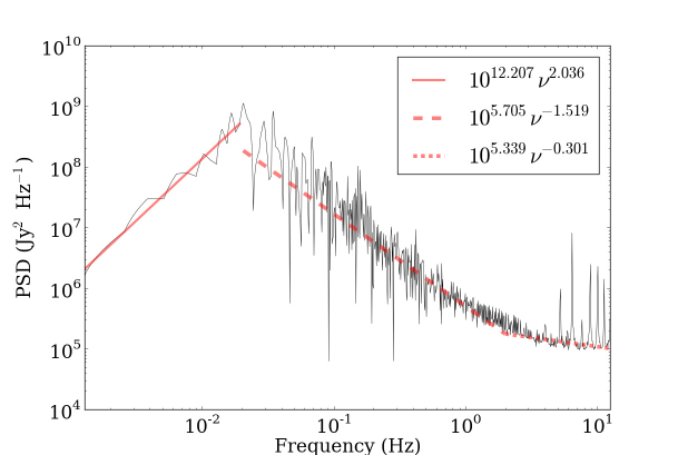
Figure 4: Fit to the raw downsampled power spectrum of a $\sim 30$ minute observation. Three independent power laws are fit to the data, with a fixed break at 0.02 Hz (below which the AC-coupled bolometer bias and readout electronics remove signal) and a fitted break at higher frequency, near 2 Hz, where the power spectrum flattens towards white noise. The beam FWHM is at about 4 Hz using the standard scan rate of 120^′′ s^-1.

The Fourier transform of the atmosphere timestream is generated by applying noise to the fitted power spectrum. The power at each frequency is multiplied by a random number sampled from a Gaussian distribution with width 1.2, determined to be a reasonable match to the data, and mean 1.0. The resulting Fourier-transformed timestream $d(t)$ is $FT(d(t))=(r_{\nu 1}P_{f})^{1/2}+i(r_{\nu 2}P_{f})^{1/2}$, where $r_{1}$ and $r_{2}$ are the normally distributed random variables and $P_{f}$ is the fitted power-law power spectrum. The atmosphere timestream is then created by inverse Fourier transforming this signal.

Gaussian noise is added to the atmospheric timestream of each bolometer independently, which renders the correlation between timestreams imperfect. This decorrelation is important for the PCA cleaning, which would remove all of the atmosphere with just one nulled component if the correlation was exact. The noise level set in the individual timestreams determines the noise level in the output map.

5.1.1 Simulated Map Parameters

We simulated the astrophysical sky by randomly sampling signal from an azimuthally symmetric 2D power-law distribution in Fourier space. The power distribution as a function of angular frequency is given by

$$P(1/r)\propto(1/r)^{-\alpha_{ps}}$$ (1)

where $r$ is the angular size-scale and $\alpha_{ps}$ is the power-law spectral index for power spectra. We modeled this signal using power spectrum power-law indices ranging from -3 to +0.5; in the HiGal $\ell=30\mbox{${}^{\circ}$}$ Science Demonstration Phase (SDP) field, the power-law index measured from the 500 $\mu\textrm{m}$ map is $\alpha_{ps}\sim 2$ over the scales of interest for comparison with Bolocam. The data were smoothed with a model of the instrument PSF to simulate the telescope’s aperture and illumination pattern. For each power-law index, three realizations of the map using different random seeds were created. The signal map was then sampled into timestreams with the Bolocam array using a standard pair of perpendicular boustrophedonic scan patterns. Examples of one of these realizations with identical random seeds and different power laws are shown in Figure 5.

Simulations performed with $\alpha_{ps}=3$ yielded no recovered astrophysical emission for normalizations in which the astrophysical sky was fainter than the atmosphere. Such a steep power spectrum is inconsistent with both BGPS and other observations: as noted above, Herschel sees structure with $\alpha_{ps}\sim 2$. The fact that the BGPS detected a great deal of astrophysical signal, none of which was brighter than the atmosphere, confirms that $\alpha_{ps}=3$ is unrealistic.

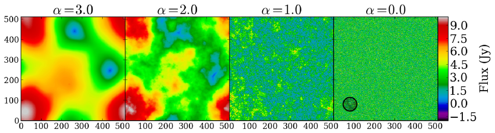
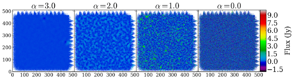
Figure 5: Examples of input (top) and output (bottom) maps for different input power-spectrum power law $\alpha_{ps}$ values. For very steep power laws, most of the power is on the largest scales. $\alpha_{ps}=0$ is white noise. The axis scales are in pixels, where each pixel is 7.2^′′, so each field is approximately 1^∘ on a side. The Bolocam footprint is plotted with a large circle of diameter 480^′′ and smaller circles of diameter 33^′′ representing each beam in its appropriate relative location. It is shown in the right panel of the top figure as an indication of the largest possible recovered angular scales; it is about 1/8th the width of the map. The input images are normalized to have the same peak flux density. The pipeline recovers no emission from the simulation with $\alpha_{ps}=3$, but this value of $\alpha_{ps}$ is not representative of the real astrophysical sky.

5.2 The Angular Transfer Function

We used a subset of these power-law simulations to measure the amount of recovered signal at each angular (spatial) scale. For each power-law in the range $1<\alpha_{ps}<2$, we used three different realizations of the map to measure the angular transfer function, defined as $STF(f)=F_{out}(f)/F_{in}(f)$ where $f$ is the angular frequency, $F_{out}$ is the azimuthally averaged power-spectrum of the pipeline-processed map, and $F_{in}$ is the azimuthally averaged power-spectrum of the simulated input map.

The angular transfer function shows only weak dependence on the ratio of astrophysical to atmospheric power, and is approximately constant at $\sim 95\%$ recovery over the range of angular scales between the beam size and $\sim 1.5\mbox{${}^{\prime}$}$. The angular transfer function is shown in Figure 6. At larger angular scales, in the range $2\mbox{${}^{\prime}$}-8\mbox{${}^{\prime}$}$, the recovery is generally low ($<80\%$). Our simulations included the full range of observed astrophysical to atmospheric flux density ratios, from $\sim 10^{-2}$ for the Central Molecular Zone (CMZ) down to $\sim 10^{-4}$ for sparsely populated regions in the $\ell\sim 70\mbox{${}^{\circ}$}$ region.

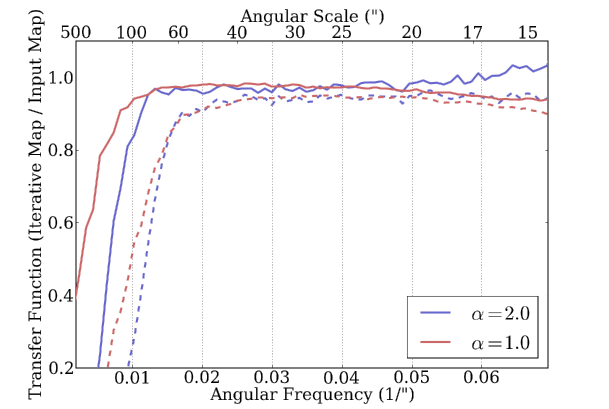
Figure 6: The angular transfer function over the range of angular scales where the BGPS data are reliable after 20 iterations (solid) and without iterative mapping (dashed). At higher angular frequency (smaller angular scale), the beam smooths out any signal. At lower angular frequency, the atmospheric subtraction removes signal. The benefits of iterative mapping in recovered flux density on all scales, but particularly the improvement in large-scale recovery, are evident. The simulations used for this measurement had a power-law sky structure with $\alpha_{ps}=2$ (blue) and $\alpha_{ps}=1$ (red).

Chapin et al. (2013) perform a similar analysis for the SCUBA-2 pipeline. Our transfer function (Figure 6) cuts off at a scale $\sim 1/6$ the SCUBA-2 scale. While the angular extent of the Bolocam footprint is only slightly smaller than SCUBA-2’s, some feature of the instrument or pipeline allows SCUBA-2 to recover larger angular scales. We speculate that the much larger number of bolometers in the SCUBA-2 array allows the atmosphere to be more reliably separated from astrophysical and internal electrical signals (bias and readout noise), so the SCUBA-2 pipeline is able to run with an atmosphere subtraction algorithm less aggressive than the 13-PCA approach we adopted.

5.3 Comparison to other data sets: Aperture Photometry

Given an understanding of the angular transfer function, it is possible to compare the BGPS to other surveys, e.g. Hi-Gal, ATLASGAL, and when it is complete, the JCMT Galactic Plane Survey (JPS), for temperature and $\beta$ measurements.

Because of the severe degeneracies in temperature/$\beta$ derivation from dust SEDs (e.g. Shetty et al. 2009b, a; Kelly et al. 2012), we recommend a conservative approach when comparing BGPS data with other data sets. For compact sources, aperture extraction with background subtraction in both the BGPS and other data set should be effective. Section 6.1 discusses aperture extraction in the presence of typical power-law distributed backgrounds.

5.4 Comparison to other data sets: Fourier-space treatment

In order to compare extended structures, which includes any sources larger than the beam, a different approach is required. The safest approach is to “unsharp mask” (high-pass-filter) both the BGPS and the other data set with a Gaussian kernel with FWHM $\lesssim 120\mbox{${}^{\prime\prime}$}$ ($\sigma\lesssim 51\mbox{${}^{\prime\prime}$}$). The filtering will limit the angular dynamic range, but will provide accurate results over the angular scales sampled.

Direct comparison of power spectra over the reproduced range is also possible. A demonstration of this approach is given in Figure 7, which shows the structure-rich $\ell=30^{\circ}$ field. The BGPS power spectrum has a shape very similar to that of HiGal. The spectral index is a commonly used measure of the ratio between flux densities at two different wavelengths in the radio,

$$\frac{F_{2}}{F_{1}}=\left(\frac{\lambda_{2}}{\lambda_{1}}\right)^{-\alpha_{\nu}}=\left(\frac{\nu_{2}}{\nu_{1}}\right)^{\alpha_{\nu}}$$ (2)

The spectral index between the BGPS at 1.1 mm and Herschel at 500 $\mu\textrm{m}$ is $\alpha_{\nu}\sim 3.7$ over the range $33\mbox{${}^{\prime\prime}$}<dx<300\mbox{${}^{\prime\prime}$}$, although because the BGPS angular transfer function is low at the large end of this range, this is only an ‘eyeball’ estimate. On the Rayleigh-Jeans tail, $\alpha_{\nu}=\beta+2$, so this spectral index is consistent with typical dust emissivity index $\beta$ measurements in the range $1.5<\beta<2$.

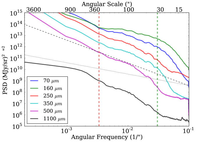
Figure 7: A comparison of the power spectra of the $\ell=30\mbox{${}^{\circ}$}$ HiGal SDP fields with the BGPS power spectrum covering the same area. The area included is 1 square degree. The dashed and dotted black lines indicate power laws with $\alpha_{ps}=2$ and $\alpha_{ps}=1$ respectively, with arbitrary normalizations, as a guide for comparison. The vertical dashed red and green lines indicate the large angular scale 50% recovery point of the BGPS (given an $\alpha_{ps}=1$ input) and the BGPS beam FWHM respectively. The ratio of 500 $\mu\textrm{m}$ to 1100 $\mu\textrm{m}$ in this example and over the marked range has a spectral index $\alpha_{\nu}\sim 3.7$. Note that the 500 $\mu\textrm{m}$ power begins falling off more steeply at $\sim 40\mbox{${}^{\prime\prime}$}$ because the Herschel FWHM beam size is $\sim 42\mbox{${}^{\prime\prime}$}$ at 500 $\mu\textrm{m}$, slightly larger than Bolocam’s (at 250 and 350 $\mu\textrm{m}$, the Herschel beam is $\sim 23\mbox{${}^{\prime\prime}$}$ and $30\mbox{${}^{\prime\prime}$}$, respectively; Traficante et al. 2011).

6 Source Extraction

Rosolowsky et al. (2010a) presented the Bolocat catalog of sources extracted from the v1.0 data with a watershed decomposition algorithm. We have used the same algorithm to create a catalog from the v2.0 catalog. We have also performed comparisons between the v1.0 and v2.0 data based on the extracted sources. The new catalog was derived using the same Bolocat parameters as in v1.0. This catalog includes regions that were not part of the v1.0 survey area, but we restrict our comparison between v1.0 and v2.0 to the area covered by both surveys.

6.1 Aperture Extraction

One major change from the v1.0 catalog is that the fluxes in the v2.0 catalog are reported with background subtracted. The backgrounds are calculated from the mode of the pixels in the range $[2R,4R]$, where R represents the aperture radius (20^′′, 40^′′, or 60^′′). The mode is computed using the IDL astrolib routine skymod.pro, which returns the mean of the selected data if the mean $\bar{\mu}$ is less than the median $\mu_{1/2}$ (indicating low “contamination” from source flux) or $3\mu_{1/2}-2\bar{\mu}$ otherwise, then performs iterative rejection of bad pixels (Landsman 1995; Stetson 1987).

We performed aperture extraction on simulated data sets to determine what size apertures are appropriate when comparing to other data sets. In Figure 8, we show the results of aperture extraction with and without background subtraction on a simulated power-law generated image with $\alpha_{ps}=2$ before and after pipeline processing. The map has had point sources added to it randomly distributed throughout the field with flux densities randomly sampled from the range $[0.1,1]$ Jy, and the power-law extended flux has an amplitude $\approx 1.8$ Jy. Sources are extracted from the pipeline-processed map using Bolocat, then the same source locations and masks are used to extract flux measurements from the input map. Figure 9 shows the input, pipeline-processed, and point-source-only maps along with the Bolocat apertures to give the reader a visual reference for an $\alpha_{ps}=2$ background with point sources. The scatter between the flux density measurements derived from the input simulated sky map and the iteratively produced map is small when background subtraction is used (the blue points), but large and unpredictable otherwise (the red points).

The agreement between the flux densities extracted from the iterative map and the input synthetic map is excellent for 40^′′ diameter background-subtracted apertures. For these apertures, the RMS of the difference between the iterative map and the input map fluxes is $\sigma=0.03$ Jy when background subtraction is used, indicating the utility and necessity of this approach. The agreement is similarly good for 80^′′ apertures ($\sigma=0.10$ Jy), but the 120^′′ apertures exhibit a source- and background-brightness dependent bias, so we recommend against apertures that large when comparing to other data sets.

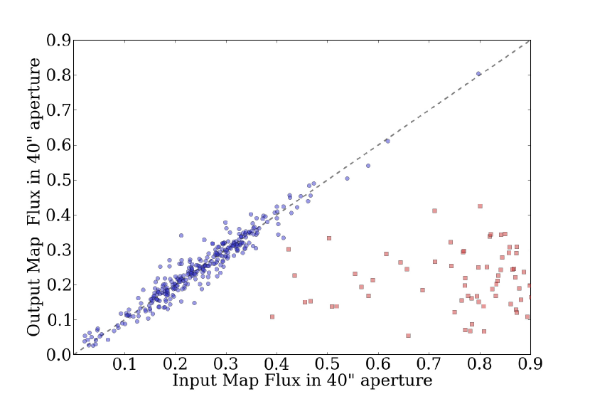
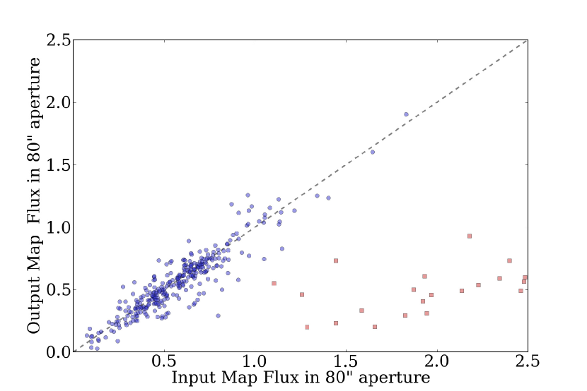
Figure 8: The aperture-extracted flux densities in a simulated map. Sources are identified from the pipeline-processed map, then flux densities are extracted from both the unprocessed input map and the pipeline-processed map. The X-axis shows the flux density of the source in the input map with (blue circles) and without (red squares) the flux density in a background annulus subtracted. Many of the red sources are not displayed as they are far to the right side of the plot, indicating poor agreement between the input and processed maps. The Y-axis shows the flux density extracted in the same aperture from the output pipeline-processed map. The black dashed line is the 1-1 line. The left plot shows 40^′′ and the right plot 80^′′ diameter apertures. Section 6 describes the background subtraction process; the v2.0 catalog reports background-subtracted flux density measurements.

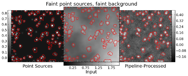
Figure 9: Images from a simulation of a power-law distributed background with $\alpha_{ps}=2$ and point sources with peak flux densities in the range $[0.1,1]$ Jy/beam. The left panel shows the pipeline-processed map, which was used to define the Bolocat masks shown as red contours. The colorbars show the flux density in units of Jy/beam. The power-law flux density distribution is evident as the structure between point sources in the left image; it is only weakly recovered by the pipeline because most of the power is on large angular scales and therefore filtered out.

There are caveats to this analysis. If the “background” power-law map has a peak flux density $\gtrsim 10\times$ the peak point-source flux density, the point sources will not be recovered: the cataloging algorithm will pick out peaks in the power law flux distribution. These cannot be analyzed with simple aperture extraction for an $\alpha_{ps}=2$ flux density distribution. However, for shallower power-law distributions, i.e. $\alpha_{ps}\lesssim 1$, aperture extraction effectively recovered accurate flux-densities in the processed maps - shallow power-law distributions more strongly resemble point-source-filled maps.

6.2 Catalog Matching between v1.0 and v2.0

We matched the v1.0 and v2.0 catalogs based on source proximity. For each source in v1.0, we identified the nearest neighbor from v2.0, and found that 5741 v2.0 sources are the nearest neighbor for a v1.0 source out of 8004 v2.0 sources in the v1.0-v2.0 overlap region. Similarly, we identified the nearest neighbor in v1.0 for each v2.0 source, finding 5745 v1.0 sources are the nearest neighbor for a v2.0 source out of 8358 v1.0 sources. There are 5538 v1.0-v2.0 source pairs for which each member of the pair has the other as its nearest-neighbor. These sources are clearly reliable and stable source identifications and constitute about 70% of the v2.0 sample.

Most of the unmatched sources have low flux density (Figure 10), but some were significantly higher - these generally represent sources that were split or merged going from v1.0 to v2.0. A few examples of how mismatches can happen are shown in Figures 11 and 12. The low-flux-density sources were most commonly unmatched in regions where the noise in v1.0 and v2.0 disagreed significantly. The high-flux-density mismatches tend to be different decompositions of bright sources and are preferentially found near very bright objects, e.g. in the Galactic center region.

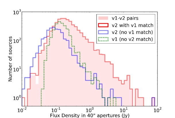
Figure 10: Histograms showing the sources matched between the v1.0 and v2.0 catalogs. Most of the v2.0 sources (5741 of 8004 v2.0 sources in the v1.0-v2.0 overlap region) have matches from v1.0, but there is a substantial population with no match. The unmatched sources tend to have lower flux densities. The shaded area shows 1-1 matches, while the solid red line shows one-way (unreciprocated) matches.

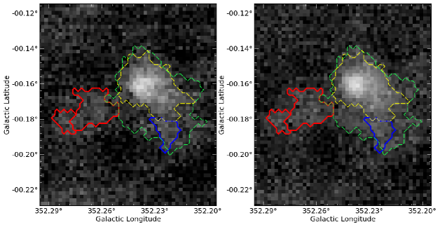
Figure 11: Contours of the extracted sources overlaid on grayscale images of a region in v1.0 (left) and v2.0 (right). The v1.0 data are scaled up by the $1.5\times$ calibration correction. The red contours show new v2.0 sources with no v1.0 match, while the blue contours show v1.0 sources with no v2.0 match. The green and yellow contours show v2.0 and v1.0 sources with a one-to-one match, respectively. In this example, the v2.0 source is significantly larger than the v1.0 source and merges with a shoulder that was classified as a separate source in v1.0. Additional v2.0 sources are detected because of increased signal-to-noise in the red-contoured regions.

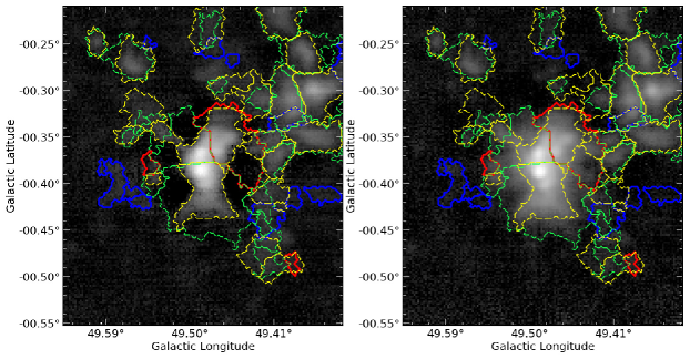
Figure 12: Same as Figure 11, but for the W51 complex. The area displayed is larger in order to encompass the entire source structure. The v2.0 sources are larger than the corresponding v1.0 sources because the negative bowl structures have been filled in. The red contours show regions where v2.0 sources were detected, but because of crowding no nearest-neighbor pair was identified in v1.0: there are more v2.0 sources than v1.0 sources. In this region, the brightest v2.0 sources are larger and brighter, but there are fewer fainter sources than in v1.0.

6.3 Source flux density, size, shape, and location distributions

We reproduce parts of Rosolowsky et al. (2010a) Figures 17 and 19 as our own Figures 13 and 14. These figures show the distributions of extracted source properties (flux density, size, and aspect ratio) for the v1.0 and v2.0 data. The source flux density distributions above the completeness cutoff are consistent between v1.0 and v2.0, both exhibiting power-law flux density distributions

$$\frac{dN}{dS_{\nu}}\propto S_{\nu}^{-\alpha_{src}}$$ (3)

with values in the range $\alpha_{src}=2.3-2.5$ for sources with $S_{\nu}\gtrsim 0.5$ Jy. In the left panel of Figure 13, we have included the v2.0 aperture-extracted data both with and without annular background subtraction. The v1.0 catalog had no background subtraction performed because the backgrounds were thought to be negligible, but the v2.0 catalog has had background subtraction performed so that the flux densities reported more accurately represent the sky. The v2.0 data include more large sources.

The longitude and latitude source flux density distribution plots, Figure 15 of Rosolowsky et al. (2010a), are reproduced in Figure 15. The properties are generally well-matched, although even with the 1.5$\times$ correction factor to the v1.0 data, there is more flux density per square degree in v2.0  sources. The gain in flux density recovery is both because of an increased flux density recovery on large angular scales and because of improved noise estimation, which results in a greater number of pixels being included in sources (see Section 6.2 for more details and Figures 11 and 12 for examples).

A two-dimensional histogram providing a broad overview of the survey contents is shown in Figure 16. The ratio of source counts per half square degree is included in panel 3. This figure illustrates that the two catalog versions are broadly consistent, and the regions in which they differ significantly tend to have fewer sources. The most extreme ratios of v2.0 to v1.0 source counts tend to occur along field edges both because of preferentially low source counts and because the v2.0 images have slightly greater extents in latitude than the v1.0.

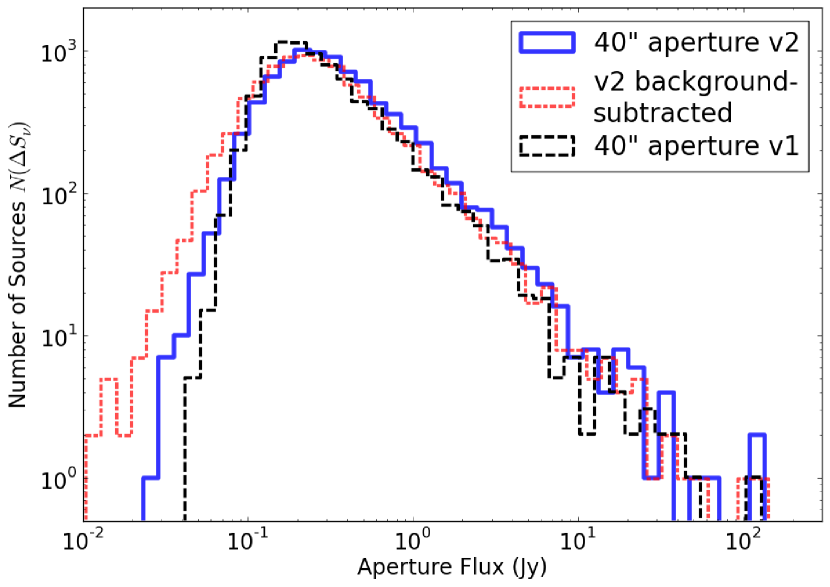
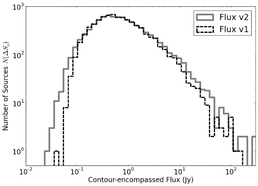
Figure 13: Comparisons of v1.0 and v2.0 flux density histograms. (left) Flux density distribution within 40^′′ diameter apertures. The 40^′′ apertures show the v2.0 data both with and without annular background subtraction; the v1.0 data are not background-subtracted. The histogram lines are slightly offset in order to minimize overlap. (right) Flux density distribution in contour-defined apertures. No background subtraction is performed for the contour-based flux densities in either version.

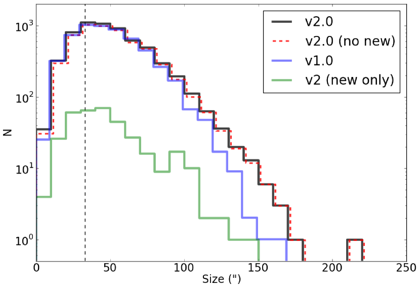
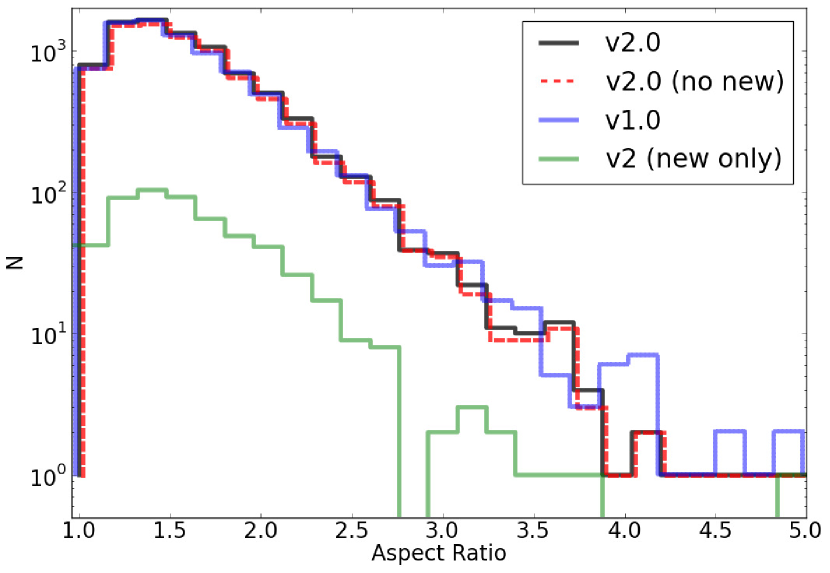
Figure 14: Distributions of deconvolved angular sizes (left) and aspect ratios (right) of sources in the BGPS catalog. The vertical dashed line in the left figure is plotted at the FWHM of the beam. The BGPS v2.0 includes newly observed regions not in the v1.0 survey, so separate histograms excluding the new (red dashed) and excluding the old (green solid) regions are shown. In both plots, the histograms are slightly offset to reduce line overlap.

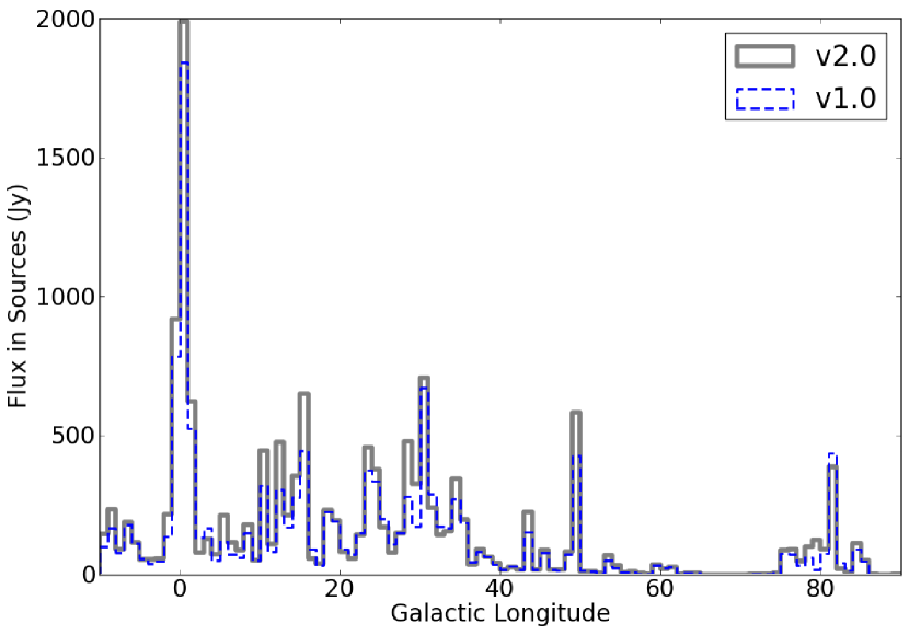
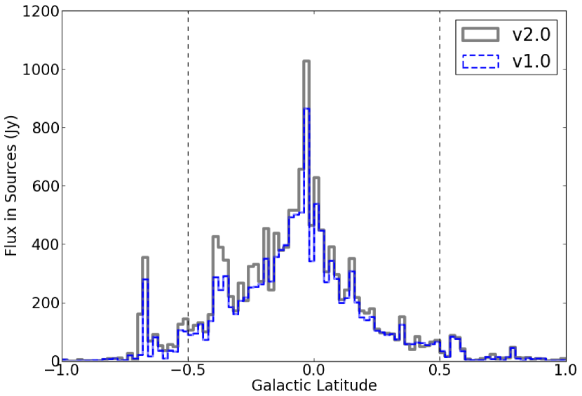
Figure 15: Distribution of total flux density in catalog sources as a function of longitude (left) and latitude (right) in the Galactic plane. The distributions contain sources extracted in the $-10\mbox{${}^{\circ}$}<\ell<90\mbox{${}^{\circ}$}$ region. (right) Vertical dashed lines indicate the extent of complete coverage in the latitude direction ($\pm 0.5\mbox{${}^{\circ}$}$). The large excess in v2.0 compared to v1.0 at $b\sim-0.4$ is due to the W51 complex, in which the flux density recovered in v2.0 was $1.5\times$ greater than in v1.0, largely because of reduced negative bowls around the brightest two sources (see Figure 12).

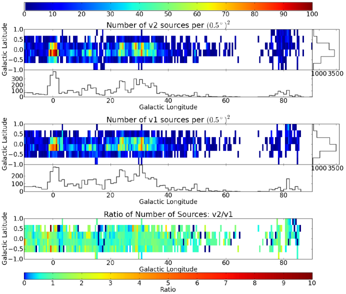
Figure 16: The two-dimensional distribution of source counts in both v1.0 and v2.0. The colors in the first two panels illustrate the number of sources per half-degree-squared bin as indicated by the top colorbar. The bottom colorbar labels the ratio of the count of v2.0 to v1.0 sources. The histograms are coarse versions of Figure 13 and show the projection of the 2D histograms along each axis. A preference toward negative-latitude sources is evident at $\ell<60\mbox{${}^{\circ}$}$, corresponding to our view of the Galaxy from slightly above the plane.

7 Conclusions

We presented Version 2 of the Bolocam Galactic Plane Survey, which is a significant improvement over v1.0 in pointing and flux calibration accuracy. The v2.0 data show an improvement in large angular scale recovery. The v2.0 release includes new observations of regions in the outer galaxy.

• We have characterized the angular transfer function of the Bolocam pipeline. Flux recovery is $>95\%$ for scales between $33\mbox{${}^{\prime\prime}$}<dx\lesssim 80\mbox{${}^{\prime\prime}$}$. The angular transfer function shows a sharp drop in recovered power above $\gtrsim 100\mbox{${}^{\prime\prime}$}$ scales.

• We compared the pointing of the BGPS to that in Hi-Gal, and found that the surveys are consistent to within the measurement error $\sigma\approx 3.5\mbox{${}^{\prime\prime}$}$.

• We measured the power spectral density in some regions and compared it to that in Hi-Gal, concluding that the power spectra are consistent with the normally used dust emissivity values in the range $\beta\sim 1.5-2$.

• A new version of the catalog has been released. The improved quality of the v2.0 images has some effects on the BGPS catalog but the basic statistical properties of the catalog have not significantly changed. Because of changing noise properties within the images, only 70% of the individual sources in v2.0 have an obvious v1.0 counterpart and vice versa. The remaining 30% of sources do not have obvious counterparts because of two effects:

  1. At low significance, changing noise levels recover different features at marginal significance. It is likely that low significance sources in v1.0 and v2.0 are both real features but have been rejected in the other catalog because of the relatively conservative limits placed on catalog membership.

  2. At high significance, the catalog algorithm is dividing up complex structure using the underlying watershed algorithm. In this case, the precise boundaries between objects are sensitive to the shape of the emission. All of the high significance features appear in both catalogs, but the objects to which a piece of bright emission is assigned can vary.

Despite these changes in the catalogs, the overall statistical properties of the population show little variation except that the largest sources appear brighter and larger owing to better recovery of the large scale flux density.

Acknowledgements: We thank the referee for a timely and constructive report. This work was supported by the National Science Foundation through NSF grant AST-1008577. The BGPS project was supported in part by NSF grant AST-0708403, and was performed at the Caltech Submillimeter Observatory (CSO), supported by NSF grants AST-0540882 and AST-0838261. The CSO was operated by Caltech under contract from the NSF. Support for the development of Bolocam was provided by NSF grants AST-9980846 and AST-0206158. ER is supported by a Discovery Grant from NSERC of Canada. NJE and MM were supported by NSF Grant AST-1109116.

References

- Aguirre et al. (2011a) Aguirre, J. E. et al. 2011a, ApJS, 192, 4
- Aguirre et al. (2011b) —. 2011b, ApJS, 192, 4
- Alexander & Kobulnicky (2012) Alexander, M. J. & Kobulnicky, H. A. 2012, ApJ, 755, L30
- Arvidsson et al. (2010) Arvidsson, K., Kerton, C. R., Alexander, M. J., Kobulnicky, H. A., & Uzpen, B. 2010, AJ, 140, 462
- Bally et al. (2010) Bally, J. et al. 2010, ApJ, 721, 137
- Battersby et al. (2011) Battersby, C. et al. 2011, A&A, 535, A128
- Battersby et al. (2010) Battersby, C., Bally, J., Jackson, J. M., Ginsburg, A., Shirley, Y. L., Schlingman, W., & Glenn, J. 2010, ApJ, 721, 222
- Berriman et al. (2004) Berriman, G. B. et al. 2004, in Astronomical Society of the Pacific Conference Series, Vol. 314, Astronomical Data Analysis Software and Systems (ADASS) XIII, ed. F. Ochsenbein, M. G. Allen, & D. Egret, 593
- Chapin et al. (2013) Chapin, E. L., Berry, D. S., Gibb, A. G., Jenness, T., Scott, D., Tilanus, R. P. J., Economou, F., & Holland, W. S. 2013, MNRAS, 430, 2545
- Chen et al. (2012) Chen, X. et al. 2012, ApJS, 200, 5
- Contreras et al. (2013) Contreras, Y. et al. 2013, A&A, 549, A45
- Dame et al. (2001a) Dame, T. M., Hartmann, D., & Thaddeus, P. 2001a, ApJ, 547, 792
- Dame et al. (2001b) —. 2001b, ApJ, 547, 792
- Dunham et al. (2011a) Dunham, M. K., Rosolowsky, E., Evans, II, N. J., Cyganowski, C., & Urquhart, J. S. 2011a, ApJ, 741, 110
- Dunham et al. (2011b) —. 2011b, ApJ, 741, 110
- Dunham et al. (2010) Dunham, M. K. et al. 2010, ApJ, 717, 1157
- Ellsworth-Bowers et al. (2013) Ellsworth-Bowers, T. P. et al. 2013, ApJ, 770, 39
- Enoch et al. (2007) Enoch, M. L., Glenn, J., Evans, II, N. J., Sargent, A. I., Young, K. E., & Huard, T. L. 2007, ApJ, 666, 982
- Enoch et al. (2006) Enoch, M. L. et al. 2006, ApJ, 638, 293
- Ginsburg et al. (2012) Ginsburg, A., Bressert, E., Bally, J., & Battersby, C. 2012, ApJ, 758, L29
- Ginsburg et al. (2011) Ginsburg, A., Darling, J., Battersby, C., Zeiger, B., & Bally, J. 2011, ApJ, 736, 149
- Guizar-Sicairos & Fienup (2008) Guizar-Sicairos, M. & Fienup, J. R. 2008, Opt. Express, 16, 7264
- Harvey et al. (2013) Harvey, P. M. et al. 2013, ApJ, 764, 133
- Ioannidis & Froebrich (2012) Ioannidis, G. & Froebrich, D. 2012, MNRAS, 421, 3257
- Jackson et al. (2006) Jackson, J. M. et al. 2006, ApJS, 163, 145
- Juvela & Ysard (2012) Juvela, M. & Ysard, N. 2012, A&A, 541, A33
- Kelly et al. (2012) Kelly, B. C., Shetty, R., Stutz, A. M., Kauffmann, J., Goodman, A. A., & Launhardt, R. 2012, ApJ, 752, 55
- Landsman (1995) Landsman, W. B. 1995, in Astronomical Society of the Pacific Conference Series, Vol. 77, Astronomical Data Analysis Software and Systems IV, ed. R. A. Shaw, H. E. Payne, & J. J. E. Hayes, 437
- Matthews et al. (2009) Matthews, H. et al. 2009, AJ, 138, 1380
- Molinari et al. (2010a) Molinari, S. et al. 2010a, A&A, 518, L100
- Molinari et al. (2010b) —. 2010b, A&A, 518, L100
- Motte et al. (2007) Motte, F., Bontemps, S., Schilke, P., Schneider, N., Menten, K. M., & Broguière, D. 2007, A&A, 476, 1243
- Pandian et al. (2012) Pandian, J. D., Wyrowski, F., & Menten, K. M. 2012, ArXiv e-prints
- Rathborne et al. (2006) Rathborne, J. M., Jackson, J. M., & Simon, R. 2006, ApJ, 641, 389
- Reiter et al. (2011) Reiter, M., Shirley, Y. L., Wu, J., Brogan, C., Wootten, A., & Tatematsu, K. 2011, ApJ, 740, 40
- Rosolowsky et al. (2010a) Rosolowsky, E. et al. 2010a, ApJS, 188, 123
- Rosolowsky et al. (2010b) —. 2010b, ApJS, 188, 123
- Sayers et al. (2010) Sayers, J. et al. 2010, ApJ, 708, 1674
- Schenck et al. (2011) Schenck, D. E., Shirley, Y. L., Reiter, M., & Juneau, S. 2011, AJ, 142, 94
- Schlingman et al. (2011) Schlingman, W. M. et al. 2011, ApJS, 195, 14
- Schuller (2012) Schuller, F. 2012, in Society of Photo-Optical Instrumentation Engineers (SPIE) Conference Series, Vol. 8452, Society of Photo-Optical Instrumentation Engineers (SPIE) Conference Series
- Schuller et al. (2009) Schuller, F. et al. 2009, A&A, 504, 415
- Shetty et al. (2009a) Shetty, R., Kauffmann, J., Schnee, S., & Goodman, A. A. 2009a, ApJ, 696, 676
- Shetty et al. (2009b) Shetty, R., Kauffmann, J., Schnee, S., Goodman, A. A., & Ercolano, B. 2009b, ApJ, 696, 2234
- Shirley et al. (2013) Shirley, Y. L. et al. 2013, ApJ
- Stetson (1987) Stetson, P. B. 1987, PASP, 99, 191
- Traficante et al. (2011) Traficante, A. et al. 2011, MNRAS, 416, 2932
- Welsch et al. (2004) Welsch, B. T., Fisher, G. H., Abbett, W. P., & Regnier, S. 2004, ApJ, 610, 1148