A model for the ESR-STM phenomenon

Abstract

We propose a model to account for the observed ESR-like signal at the Larmor frequency in the current noise STM experiments identifying spin centers on various substrates. The theoretical understanding of this phenomenon, which allows for single spin detection on surfaces at room temperature, is not settled for the experimentally relevant case that the tip and substrate are not spin polarized. Our model is based on a direct tip-substrate tunneling in parallel with a current flowing via the spin states. We find a sharp signal at the Larmor frequency even at high temperatures, in good agreement with experimental data. We also evaluate the noise in presence of an ac field near resonance and predict splitting of the signal by the Rabi frequency.

Observing and manipulating single spins is of considerable interest in quantum information. A particularly promising method of detecting a single spin on a surface is by using a Scanning Tunneling Microscope (STM) review . The technique has been initiated and developed by Y. Manassen and various collaborators and has the appealing feature of being useful at ambient conditions, in contrast to other techniques operating at very low temperatures lowt . It is based on monitoring the noise, i.e. the current-current correlations, in the STM current and observing a signal at the expected Larmor frequency, similar to an Electron Spin Resonance (ESR) experiment, except that here no oscillating field is applied. The frequency of the signal varies linearly with the applied magnetic field, confirming that the STM in fact detects an isolated spin on the surface. This phenomenon was demonstrated on oxidized Si(111) surface manassen1 ; manassen2 . Afterwards it was also observed in Fe atoms manassen3 on Si(111) as well as on a variety of organic molecules on a graphite surface durkan and on Au(111) surfaces messina ; mannini ; mugnaini . Recent extensions have resolved two resonance peaks on oxidized Si(111) $7\times 7$ surface corresponding to site specific $g$ factors komeda ; sainoo and also enabled the observation of the hyperfine coupling review ; manassen4 .

The theoretical understanding of the ESR-STM effect is not settled review . The emergence of a finite frequency in a steady state stationary situation is a non-trivial phenomenon. An obvious mechanism for coupling the charge current to the spin precession is spin-orbit coupling mozyrsky . It was shown, that an ESR signal is present in the noise of systems with spin-orbit coupling only when the leads are polarized, either for a strong Coulomb interaction bulaevskii ; gurvitz or for the non-interacting case gurvitz . This was shown even in linear response entin . However, it was found that the signal vanishes when the lead polarization vanishes or with parallel polarizations. In the experiments the leads are very weakly polarized by the magnetic field with polarization parallel to that of the localized spin, hence the ESR signal vanishes within these models bulaevskii ; gurvitz . It was argued that an effective spin polarization is realized as a fluctuation effect either for a small number of electrons that pass the localized spin in one cycle balatsky or due to 1/f magnetic noise of the tunneling current manassen5 . It was further shown that spin-orbit coupling in an asymmetric dot can yield an oscillating electric dipole, possibly affecting the STM current levitov .

In the present work we start by showing that the problem of tunneling via spin states in the presence of spin-orbit interaction has strictly no resonance signal; the presence of an electric dipole coupling does not change this conclusion. We then study a model in which an additional direct coupling between the dot and the reservoir is included. Our model is motivated by studies of quantum dots with spin-orbit lopez and by STM studies of a two-impurity Kondo system that shows a significant direct coupling between the tip and substrate states bork ; hamad . We find that the interference of the direct current and the one via the spin does show an ESR signal in the noise, which increases with the direct coupling. This feature is consistent with the unusual non-monotonic contour plot presented in Refs. manassen1, ; manassen2, , i.e. the signal is maximized when the STM tip is not directly on the spin center but slightly ($\sim 1$nm) away, so as to maximize an overlap with a surface state of the substrate. The signal intensity relative to the background is small, yet it is sharp even at temperatures much higher than the ESR frequency; the consistency of this behavior with the experimental data is discussed below. Finally, we also evaluate the noise in presence of an ac field near resonance and predict splitting of the signal.

The setup we consider consists of a molecule $M$ with spin $1/2$ on a metallic substrate and also in contact with an STM tip. The tip and the substrate define two electron reservoirs $T,S$. The two states of the molecule, associated to the two spin orientations of the molecule have energies separated by a Zeeman splitting due to an external magnetic field ${\bf B}=B\hat{e}_{z}$, and are coupled by tunneling processes to the two reservoirs. We assume, in addition, spin-orbit (SO) coupling, which renders these tunneling terms spin dependent, in particular allowing for tunneling with spin-flip. The Hamiltonian is

$${\cal H}=\sum_{\alpha=T,S}{\cal H}_{\alpha}+{\cal H}_{M}+\sum_{\alpha=T,S}{\cal H}_{M,\alpha}.$$ (1)

The first term, with ${\cal H}_{\alpha}=\sum_{k\alpha,\sigma}\varepsilon_{k{\alpha}}c^{\dagger}_{k{\alpha},\sigma}c_{k{\alpha},\sigma}$, corresponds to the unpolarized reservoirs. The molecule is described by the simple model

$${\cal H}_{M}=\sum_{\sigma=\pm}\varepsilon_{\sigma}d^{\dagger}_{\sigma}d_{\sigma},$$ (2)

with the energy of two spin orientations separated by the Zeeman splitting $\varepsilon_{\pm}=\pm\omega_{z}$/2. The last term of ${\cal H}$ is the coupling to the reservoirs,

$${\cal H}_{M,\alpha}=w\sum_{k{\alpha},\sigma,\sigma^{\prime}}\left[c^{\dagger}_{k{\alpha},\sigma}U_{\sigma,\sigma^{\prime}}^{\alpha\dagger}d_{\sigma^{\prime}}+H.c\right],$$ (3)

where $U^{\alpha}$ are unitary matrices for $\alpha=T,S$.

Let us now notice that the above Hamiltonian does not contain the minimum ingredients to describe the ESR-STM effect. In fact, the unitary transformation $c_{k\alpha,\sigma}^{\prime}=\sum_{\sigma^{\prime}}U_{\sigma,\sigma^{\prime}}^{\alpha}c_{k\alpha,\sigma^{\prime}}$ diagonalizes in spin the tunneling Hamiltonian while leaves unchanged the Hamiltonians of the unpolarized reservoirs. The result is ${\cal H}_{M,\alpha}=w\sum_{k{\alpha},\sigma}[c^{\prime\dagger}_{k{\alpha},\sigma}d_{\sigma}+H.c]$. Hence, the full Hamiltonian is a sum over two decoupled spin states and observables such as current noise cannot present any feature depending on the level spacing in the molecule, as previously noted in a detailed calculation gurvitz .

The next ingredient to explore is a molecular electric dipole $e{\bf r}$ that couples to an electric field ${\bf E}$, e.g. due to tip proximity levitov . Assuming a molecule with several levels, in the absence of ${\bf E}$, ${\cal H}_{M}$ has eigenstates $|m,\sigma\rangle$ with eigenvalues $E_{m}\pm\mbox{\small$\frac{1}{2}$}\omega_{z,m}$ ($m=0$ is the ground state) where $\omega_{z,m}$ is the splitting due to a Zeeman term ${\cal H}_{Z}$. Extending the one-dimensional model levitov , the oscillating electric dipole $\sim\mbox{e}^{-i\omega_{z,0}t}$ can be described by the 2nd order matrix element

$$\sum_{m\neq 0}\frac{\langle 0,-|{\bf E}\cdot{\bf r}|m,-\rangle\langle m,-|{\cal H}_{Z}|0,+\rangle}{E_{0}-E_{m}},$$ (4)

where the asymmetry of the molecule allows for $\langle m,-|{\cal H}_{Z}|0,+\rangle\neq 0$ for $m\neq 0$. Adding this off-diagonal term to ${\cal H}_{M}$ results in eigenstates related to $|0,\pm\rangle$, i.e. $d_{\sigma}$, by a unitary spin rotation. Therefore Eqs. (2) and (3) retain their structure, the spin states decouple and no ESR-STM effect, hence some additional modulation of the tunnel barrier is needed levitov .

Then, we keep considering the simple Hamiltonian (2) for the molecule and we proceed to introduce the main feature of our model. Namely, a direct tunneling between the tip and substrate so that the Hamiltonian (1) acquires an additional term

$${\cal H}_{TS}=W\sum_{kT,k^{\prime}S,\sigma,\sigma^{\prime}}\left[c_{kT,\sigma}^{\dagger}U_{\sigma,\sigma^{\prime}}^{TS}c_{k^{\prime}S,\sigma^{\prime}}+H.c.\right]$$ (5)

In terms of the operators $c^{\prime}_{k\alpha,\sigma}$ previously defined, ${\cal H}_{TS}$ involves the unitary matrix ${\tilde{U}}=U^{T}U^{TS}U^{S\dagger}$ which can be written as a general rotation of the form ${\tilde{U}}=U^{\rm SO}{U}^{S}$ with $U^{\rm SO}=\mbox{e}^{i\sigma_{z}\phi_{1}/2}$, and $U^{S}=\mbox{e}^{i\sigma_{z}\phi_{2}/2}\mbox{e}^{i\sigma_{y}\theta/2}\mbox{e}^{-i\sigma_{z}\phi_{2}/2}$, where $\sigma_{x,y,z}$ the Pauli matrices. We note that with $\theta=0$ the spin states decouple, hence $\theta\neq 0$ is essential for the ESR effect. In terms of the unitary transformation $c^{\prime\prime}_{kT,\sigma}=\sum_{\sigma^{\prime}}{\hat{U}}^{S}_{\sigma,\sigma^{\prime}}c^{\prime}_{kS,\sigma^{\prime}}$ the direct $TS$ coupling becomes spin diagonal with the matrix $U^{SO}$ while ${\cal H}_{M,S}$ becomes off diagonal with ${\hat{U}}^{S}$. The phase $\phi_{2}$ can be eliminated by defining $d_{\sigma}=\mbox{e}^{i\sigma\phi_{2}/2}{\tilde{d}}_{\sigma}$, $c^{\prime}_{kT,\sigma}=\mbox{e}^{i\sigma\phi_{2}/2}{\tilde{c}}_{kS,\sigma}$ and $c^{\prime\prime}_{kS,\sigma}=\mbox{e}^{i\sigma\phi_{2}/2}{\tilde{c}}_{kS,\sigma}$. The different Hamiltonian terms become

$${\cal H}_{TS} = W\sum_{kT,k^{\prime}S,\sigma}[{\tilde{c}}^{\dagger}_{kT,\sigma}\mbox{e}^{i\sigma\phi_{1}}{\tilde{c}}_{k^{\prime}S,\sigma}+H.c.]$$

$${\cal H}_{M,S} = w\sum_{kS,\sigma}[{\tilde{c}}^{\dagger}_{kS,\sigma}{\tilde{d}}_{\sigma}+H.c.]$$

$${\cal H}_{M,T} = w\sum_{kT,\sigma,\sigma^{\prime}}[{\tilde{c}}^{\dagger}_{kT,\sigma}\left(\mbox{e}^{i\sigma_{y}\theta/2}\right)_{\sigma,\sigma^{\prime}}{\tilde{d}}_{\sigma^{\prime}}+H.c.]$$ (6)

while the ${\cal H}_{T},{\cal H}_{S}$ terms of (1) remain unchanged with the ${\tilde{c}}_{k\alpha,\sigma},{\tilde{d}}_{\sigma}$ operators.

For this model, the charge current operator flowing into the tip reads $\hat{J}_{T}(t)=\hat{J}_{M\rightarrow T}(t)+\hat{J}_{S\rightarrow T}(t)$, where the first term corresponds to the current flowing through the molecule, while the second one is due to the direct tunneling $W$. We expect the T-M capacitance to be smaller than the M-S one birk , hence the circuit current but is dominated by the tip current $\hat{J}_{T}$. The corresponding noise spectrum can be decomposed as ${\cal S}(t,\omega)={\cal S}_{M}(t,\omega)+{\cal S}_{W}(t,\omega)$. The first term corresponds to current-current correlation functions involving current operators through the molecule, while the second one corresponds to those due to the direct current between tip and substrate,

$${\cal S}_{M}(t,\omega) = \int_{-\infty}^{+\infty}d\tau\langle\hat{J}_{T}(t)\hat{J}_{M\rightarrow T}(t-\tau)+$$

$$\hat{J}_{M\rightarrow T}(t)\hat{J}_{T}(t-\tau)\rangle e^{i\omega\tau},$$

$${\cal S}_{W}(t,\omega) = 2\int_{-\infty}^{+\infty}d\tau\langle\hat{J}_{S\rightarrow T}(t)\hat{J}_{S\rightarrow T}(t-\tau)\rangle e^{i\omega\tau}.$$ (7)

In what follows we focus on the first term, which contains the relevant information involving the scattering processes through the molecule. The second one represents a background signal, which is usually subtracted from the experimental data. The current is induced by applying a dc bias voltage $V$, which relates the chemical potentials of the tip and substrate as $\mu_{T}=\mu_{S}+eV$. In this stationary case ${\cal S}_{l}(t,\omega)\equiv{\cal S}_{l}(\omega)$, $l=W,M$.

Consider now the experimentally relevant parameters. The DC current $I=\langle\hat{J}_{T}\rangle\sim 0.1-1$nA for $V\approx 1$V review . In our model we find that the Larmor frequency appears in the noise when $W\gg w$, hence the DC conductance is dominated by the $W$ term. The latter is ferrer $G_{W}=\frac{2e^{2}}{h}\frac{4x}{(1+x)^{2}}$, where $x=\pi^{2}W^{2}N_{T}N_{S}$ and $N_{T,S}$ are the tip and substrate density of states, taken as constants in the $(\mu_{T},\mu_{S})$ range. Assuming $N_{T,S}\sim 1/b$, where $b$ is the bandwidth of these reservoirs, we estimate $W/b\approx 10^{-3}$ corresponding to a weak tunneling regime with $x\ll 1$. The resonance is sharp, with a width of review $\Delta\omega/2\pi\approx 1$MHz, much smaller than the resonance frequency, typically $\omega_{z}/2\pi\approx 500$MHz. A golden rule estimate, consistent with our data for small $w,W$, gives a resonance width $\Delta\omega=2\pi w^{2}/b$. The ensuing estimate for the DC current via the molecule is $\langle J_{M\rightarrow T}\rangle=2e\Delta\omega/2\pi$. The $\Delta\omega$ value above yields $\sim 10^{-12}$A, verifying that the DC current is indeed dominated by the direct conductance $G_{W}$. Considering $b\approx 5eV$ we estimate $w/b\approx 10^{-5}$. We note that the experiments were at room temperature, $T\gg\omega_{z}$, hence the linewidth is not sensitive to temperature. We assume that the chemical potential of the substrate $\mu_{S}=0$ lies between the two levels. Our results depend weakly on the position of these levels, as long as at least one of them is in between $\mu_{S}$ and $\mu_{R}$.

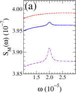
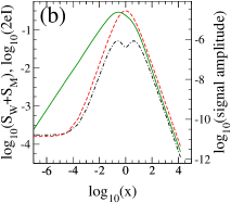
Figure 1: (Color online) (a) noise spectrum ${\cal S}_{M}$ for various direct couplings $W$ between reservoirs: 0 (dashed red), 0.05 (solid blue) and 0.1 (dash-dotted violet). Parameters are: $\mu_{T}=0.5$, $\mu_{T}=0$, $T=0.05$, $w=5\cdot 10^{-4}$, $\epsilon_{\pm}=\pm 10^{-5}$ and b=5. (b) amplitude of the signal at the Larmor frequency (solid green), the background noise ${\cal S}_{W}+{\cal S}_{M}$ (dot-dashed black) and $2eI$ (dashed red) as functions of $x$. Parameters are $w=0.01$, $\epsilon_{\pm}=\pm 5\cdot 10^{-3}$, other parameters as in (a).

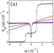
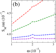
Figure 2: (Color online) Noise spectrum ${\cal S}_{M}$ at various temperatures $T$: 0 (black triangles down), $5\cdot 10^{-5}$ (red triangles up), $10^{-4}$ (green diamond), $5\cdot 10^{-4}$ (blue squares), and $5\cdot 10^{-3}$ (violet circles). Parameters are: $W=0.1$ and those in Fig 1a. (b) shows a magnified part of (a) in the resonance vicinity.

We now show results for the noise spectrum in our model. We have calculated ${\cal S}_{M}(\omega)$ and ${\cal S}_{T}(\omega)$ following the procedure of Ref. noise0, . We use $\theta=\pi$ and $\phi_{1}=\pi/2$ to maximize the resonance effect, (the value of $\phi_{1}$ is irrelevant to the resonance effect). We chose $W,w,T,eV,\epsilon_{\pm}$ not too far from the experimental estimates (in eV units). Both reservoirs are modeled as semi-infinite 1D chains with bandwidth $b$ so that $x=(4W/b)^{2}$.

Fig. 1a shows the onset of the Larmor frequency in the noise ${\cal S}_{M}$ as the direct coupling $W$ is turned on. We have studied the effect of $w$ on this resonance and extended the model to different tunneling coupling to the tip and substrate $w_{S}$ and $w_{T}$, respectively. We found that the the width (as expected above for $w_{T}=w_{S}$) as well as the amplitude scale as $w_{S}w_{T}$. In Fig. 1b we show the amplitude of the signal as a function of $x$, the background noise and the classical shot noise $2eI$. The background noise is taken as the mean in the range $\omega_{z}\pm 0.1\omega_{z}$, where the noise varies by less than $1\%$. We note that for $x\ll 1$ or $x\gg 1$ the background is the classical shot noise ${\cal S}_{W}+{\cal S}_{M}\approx 2eI$. The current ratio is $\langle J_{M\rightarrow T}\rangle/\langle J_{S\rightarrow T}\rangle\approx 4\pi w^{2}/(bxeV)$ (for $x\ll 1$) which for the parameters of Fig. 1b is $\approx 10^{-4}/x$. Hence at $x<10^{-4}$ the current, as well as the background noise, is dominated by that via the molecule and becomes $x$ independent. The case $x=1$ corresponds to perfect ballistic matching between the reservoirs, accounting for the maxima in the figure.

Fig. 1b shows that the signal intensity at $x\ll 1$ is linear with $x$, same as ${\cal S}_{W}\sim G_{W}\sim x$. The signal to background ratio at $x=0.01$ is $\sim 10^{-3}$. Scaling to $w=5\cdot 10^{-5}$ reduces this ratio to $\sim 10^{-8}$. For this $w$ the background is $S_{W}$ dominates, hence the ratio above is $x$ independent and applies to the experimental situation.

The temperature dependence is shown in Fig. 2. The resonance itself is not sensitive to temperature (see Fig. 2b), consistent with the experimental data review . In the case of $T=0$ there are features of the noise spectrum (steps) at the frequencies corresponding to the molecular levels $\varepsilon_{\pm}$, which are typical of the noise spectrum of two-level systems rothstein . These features are washed up by thermal fluctuations as soon as $T>\omega_{z}$. The dip at $\omega=0$ is similar to the one seen in Ref. rothstein, , with the latter due to charge conservation at the molecule.

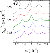
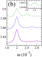
Figure 3: (Color online) (a) noise spectrum ${\cal S}^{\rm dc}_{M}$ for perpendicular ac field amplitude $\Delta_{\perp}=5\cdot 10^{-6}$ and various frequencies $\Omega_{0}$: $1.9\cdot 10^{-5}$ (long-dashed black), $1.94\cdot 10^{-5}$ (dashed red), $2\cdot 10^{-5}$ [resonant] (solid green), $2.06\cdot 10^{-5}$ (dashed-dotted blue), and $2.1\cdot 10^{-5}$ (long-dashed-dotted violet). (b) noise spectrum ${\cal S}^{\rm dc}_{M}$ for parallel ac field amplitude $\Delta_{\parallel}=2\cdot 10^{-6}$ and various frequencies $\Omega_{0}$: $4\cdot 10^{-6}$ (dashed-dotted green), $6\cdot 10^{-6}$ (dashed blue), and $8\cdot 10^{-6}$ (solid violet). Inset: second harmonic corresponding to $\Omega_{0}=4\cdot 10^{-6}$. Parameters are: $W=0.1$ and those in Fig. 1a. The curves below the top one in (a) and (b) are displaced in height for clarity.

In Fig. 3a we show the noise in presence of an additional ac magnetic field perpendicularly applied with respect to ${\bf B}$, $B_{\perp}(t)=\Delta_{\perp}\cos(\Omega_{0}t)\sigma_{1}$ that induces transitions between the molecule levels. For the isolated molecule the transition amplitude at time $t$ is

$$\langle-,t|+,t=0\rangle=\frac{\Delta_{\perp}}{a}\mbox{e}^{-\mbox{\small$\frac{1}{2}$}i\Omega_{0}t}\sin(\mbox{\small$\frac{1}{2}$}at)$$ (8)

where $a=\sqrt{(\Omega_{0}-\omega_{z})^{2}+\Delta_{\perp}^{2}}$ is the Rabi frequency. In the presence of $B_{\perp}(t)$, the current-current correlation functions (A model for the ESR-STM phenomenon) depend on the time argument $t$. In what follows we consider the ensuing dc components

$${\cal S}^{\rm dc}_{l}(\omega)=\frac{\Omega_{0}}{2\pi}\int_{0}^{\Omega_{0}/(2\pi)}dt{\cal S}_{l}(t,\omega).$$ (9)

In the present case, we resort to the non-equilibrium Green function formalism of Refs. noiset, to evaluate this function. Fig. 3a shows splitting of the line into three signals located at $\Omega_{0}$ and $\Omega_{0}\pm a$. The amplitudes of the signals increase as the satellite peaks become closer to $\omega_{z}$. In usual ESR one usually observes the average spin with a resonance at $\omega_{z}$ while the amplitude of the Rabi frequency $a$ decays by a $T_{2}$ process. The analog of our current correlation is, however, the spin-spin correlation in ESR. The latter is in fact related to light scattering from a 2-level system showing a “Mollow triplet” muller ; ulrich .

In Fig. 3b we show the noise in presence of an ac magnetic field parallel to ${\bf B}$, $B_{\parallel}(t)=\Delta_{\parallel}\cos(\Omega_{0}t)\sigma_{z}$ which produces an oscillation in the energy levels around their equilibrium values with amplitude $\Delta_{\parallel}$ and frequency $\Omega_{0}$. In this case, the time evolution of the off diagonal $\sigma_{1}$ element is

$$e^{i\int_{0}^{t}(\omega_{z}+\Delta_{\parallel}\cos(\Omega_{0}t^{\prime}))dt^{\prime}}=e^{i\omega_{z}t}\sum_{n=-\infty}^{\infty}J_{n}\left(\frac{\Delta_{\parallel}}{\Omega_{0}}\right)e^{in\Omega_{0}t}$$ (10)

where $J_{n}(x)$ are the Bessel functions. For $\Delta_{\parallel}\ll\Omega_{0}$ only the first terms of the series with $n=0,\pm 1$ contribute being the term with $n=0$ with $J_{0}(0)=1$ the dominant one. Thus, in remarkable contrast with the case of a perpendicular ac field, the strongest noise signal appears at $\omega_{z}$ with two sizable satellites at $\omega_{z}\pm\Omega_{0}$. This is illustrated in Fig. 3b, where the main peak and the right satellite are shown for several values of $\Omega_{0}$; the inset zooms on the weaker second order order satellite at $\omega_{z}+2\Omega_{0}$. A case with many sidebands was in fact studied by ERS-STM manassen3 and is consistent with Eq. (10). It is remarkable that these well known features from ESR are reproduced in the current noise spectra.

Discussion: Our model assumes that the spin-orbit interaction is significant, for at least one of the tunneling terms. We note that the strong electric field near the tip can enhance the spin-orbit coupling in the molecule. We consider now several unusual features of the data that our model can account for: (i) A sharp resonance even at high temperatures $T\gg\omega_{z}$, (ii) insensitivity to the details of the spin defect, i.e. to the positions of its levels between the tip and substrate chemical potentials, (iii) contour plots manassen1 ; manassen2 showing that the signal is maximal at $\sim 1$nm from a center, hence a significant direct coupling $W$ bypassing the spin can be achieved. (iv) We account for the ESR-STM phenomenon with unpolarized tip or substrate, in contrast with previous models bulaevskii ; gurvitz that require polarized leads.

We note that the background noise is not measured in the experiment since the modulation technique review measures the derivative of the noise spectra. Furthermore, the signal intensity is under study manassen4 as it is highly sensitive to uncertainties in the feedback and impedance matching circuits. We estimate that the signal to background intensity is $\sim 10^{-8}$ as discussed above. Furthermore, we predict the appearance of triplet lines when adding a time dependent field perpendicular to the DC one. The spacing of these lines is determined by the Rabi frequency. We also predict multiple sidebands for modulation with parallel field, partly seen in experiment manassen3 . In conclusion, our model presents a solution to a long standing puzzle, paving the way for more controlled single spin detection via ESR-STM.

- (1) A. V. Balatsky, M. Nishijima and Y. Manassen, Adv. Phys. 61, 117 (2012).
- (2) D. Rugar, R. Budakian, H. J. Mamin, and B. W. Chui, Nature 430, 329 (2004).
- (3) Y. Manassen, R.J. Hamers, J.E. Demuth, and A.J. Castellano Jr., Phys Rev. Lett. 62, 2531 (1989).
- (4) Y. Manassen, E. Ter-Ovanesyan, D. Shachal, and S. Richter, Phys. Rev. B 48, 4887 (1993).
- (5) Y. Manassen, I. Mukhopadhyay, and N. Ramesh Rao, Phys. Rev. B 61, 16223 (2000).
- (6) C.Durkan and M. E. Welland, Appl. Phys. Lett. 80, 458 (2002).
- (7) P. Messina, M. Mannini, A. Caneschi, D. Gatteschi, L. Sorace, P. Sigalotti, C. Sandrin, P. Pittana and Y Manassen, J. Appl. Phys. 101, 053916 (2007).
- (8) M. Mannini, P. Messina, L. Sorace, L. Gorini, M. Fabrizioli, A. Caneschi, Y. Manassen, P. Sigalotti, P. Pittana and D. Gatteschi, Inorganica Chimica Acta 360, 3837 (2007).
- (9) V. Mugnaini, M. Fabrizioli, I. Ratera, M. Mannini, A.Caneschi, D. Gatteschi, Y. Manassen and J. Veciana, Sol. St. Sci. 11, 956 (2009).
- (10) T. Komeda and Y. Manassen, Appl. Phys. Lett. 92, 212506 (2008).
- (11) Y. Sainoo, H. Isshiki, S.M.F. Shahed, T. Takaoka and T. Komeda, Appl. Phys. Lett. 95, 082504 (2009).
- (12) Y. Manassen, M. Averbukh and M. Morgenstern (unpublished); and Y. Manassen, private communication.
- (13) D. Mozyrsky, L. Fedichkin, S. A. Gurvitz and G. P. Berman, Phys. Rev. B 66, 161313 (2002)
- (14) L. N. Bulaevskii, M. Hruska and G. Ortiz, Phys. Rev. B 68, 125415 (2003).
- (15) S. A. Gurvitz, D. Mozyrsky and G. P. Berman, Phys. Rev. B 72, 205341 (2005).
- (16) O. Entin-Wohlman, Y. Imry, S. A. Gurvitz, and A. Aharony, Phys. Rev. B 75, 193308 (2007).
- (17) A. V. Balatsky, Y. Manassen and R. Salem, Phil. Mag. B 82, 1291 (2002); Phys. Rev. B 66, 195416 (2002).
- (18) Y. Manassen and A. V. Balatsky, Special issue on single molecule spectroscopy: Israel Journal of Chemistry 44, 401 (2004) [Cond-mat/0402460].
- (19) L. S. Levitov and E. I. Rashba, Phys. Rev. B 67, 115324 (2003).
- (20) R. López, D. Sánchez and L. Serra, Phys. Rev. B 76, 035307 (2007).
- (21) J. Bork, Y. Zhang, L. Diekhöner, L. Borda, P. Simon, J. Kroha, P. Wahl and K. Kern, Nature Phys. 7, 901 (2011).
- (22) I. J. Hamad, L. Costa Ribeiro, G. B. Martins, E. V. Anda, Phys. Rev. B 87, 115102 (2013).
- (23) H. Birk, M. J. M. de Jong and C. Schönenberger, Phys. Rev. Lett. 75, 1610 (1995).
- (24) Ya. M. Blanter and M. Büttiker, Phys. Rep. 336, 1 (2000).
- (25) J. Ferrer, A. Martín-Rodero and F. Flores, Phys. Rev. B 38, 10113 (1988).
- (26) B. Rizzo, L. Arrachea, and J. P. Paz, Phys. Rev. B 85, 045442 (2012).
- (27) A. Caso. L. Arrachea and G. Lozano, Eur. Phys. Jour. B 85, 266 (2012); L. Arrachea, Phys. Rev. B 75, 035319 (2007).
- (28) E. A. Rothstein, O. Entin-Wohlman and A. Aharony, Phys. Rev. B 79, 075307 (2009).
- (29) A. Muller, E. B. Flagg, P. Bianucci, X.Y. Wang, D. G. Deppe, W. Ma, J. Zhang, G. J. Salamo, M. Xiao and C. K. Shih, Phys. Rev. Lett. 99, 187402 (2007).
- (30) S. M. Ulrich, S. Ates, S. Reitzenstein, A. Löffler, A. Forchel and P. Michler, Phys. Rev. Lett. 106, 247402 (2011).