Generalized Plasma Dispersion Function: One-Solve-All Treatment, Visualizations, and Application to Landau Damping

Abstract

A unified, fast, and effective approach is developed for numerical calculation of the well-known plasma dispersion function with extensions from Maxwellian distribution to almost arbitrary distribution functions, such as the $\delta$, flat top, triangular, $\kappa$ or Lorentzian, slowing down, and incomplete Maxwellian distributions. The singularity and analytic continuation problems are also solved generally. Given that the usual conclusion $\gamma\propto\partial f_{0}/\partial v$ is only a rough approximation when discussing the distribution function effects on Landau damping, this approach provides a useful tool for rigorous calculations of the linear wave and instability properties of plasma for general distribution functions. The results are also verified via a linear initial value simulation approach. Intuitive visualizations of the generalized plasma dispersion function are also provided.

I Introduction

In a one-dimensional, one-species, non-relativistic electrostatic plasma system, the Langmuir wave dispersion relation isNicholson1983

$$D(k,\omega)=1-\frac{\omega_{p}^{2}}{k^{2}}\int_{C}\frac{\partial f_{0}/\partial v}{v-\omega/k}dv=0,$$ (1)

where $k$ is the wave vector, $\omega=\omega_{r}+i\gamma$ is the frequency, $\omega_{p}=\sqrt{4\pi n_{0}q^{2}/m}$ is the plasma frequency and $C$ is the Landau integral contour.

For Maxwellian distribution $f_{0}=F_{M}$, with

$$F_{M}(v)=\frac{1}{\sqrt{\pi}v_{t}}e^{-\frac{v^{2}}{v_{t}^{2}}},$$ (2)

the well-known plasma dispersion function (PDF)

$$Z_{M}(\zeta)=\frac{1}{\sqrt{\pi}}\int_{-\infty}^{\infty}\frac{e^{-z^{2}}}{z-\zeta}dz,~{}~{}~{}\Im(\zeta)>0,$$ (3)

with analytic continuation to $\Im(\zeta)\leq 0$, is defined by Fried and ConteFried1961 , where $\zeta=\omega/(kv_{t})$ and $z=v/v_{t}$. Hence, (1) is rewritten to

$$D(k,\omega)=1-\frac{1}{(k\lambda_{D})^{2}}\frac{1}{2}Z^{\prime}_{M}(\zeta)=0,$$ (4)

with also

$$Z^{\prime}_{M}(\zeta)=-2[1+\zeta Z_{M}(\zeta)],$$ (5)

where $\lambda_{D}=\sqrt{T/m}/\omega_{p}$ and $v_{t}=\sqrt{2T/m}$. A $\sqrt{2}$ difference in the normalizations between $v_{t}$ and $T$ should be noted.

Analytic properties and numerical approaches for the usual PDF (3), which is similarly related to complex error function, Faddeeva function, or Dawson integral, have been extensively studied since Fried and ConteFried1961 . Good $Z_{M}(\zeta)$ function numerical schemes for practical application can also be easily found. However, in studying other distribution functions, it should be treated separately. The singularity in real line and analytic continuation to $\Im(\zeta)\leq 0$ usually requires careful treatment, otherwise it would be confusing and would yield incorrect results.

A family of distributions, i.e., $\kappa$ distributions or generalized Lorentzian distributionsValentini2007

$$F_{\kappa}=A_{\kappa}\Big{[}1+\frac{1}{\kappa}\frac{v^{2}}{v_{t}^{2}}\Big{]}^{-\kappa},$$ (6)

with the normalization constant

$$A_{\kappa}=\frac{1}{v_{t}}\frac{\Gamma(\kappa)}{\Gamma(\kappa-1/2)}\frac{1}{\sqrt{\pi\kappa}},$$ (7)

are very useful for space and astrophysical plasma and have been studied intensively since Summers and ThorneSummers1991 , where $\Gamma$ is the Euler gamma function. Recently, BaalrudBaalrud2013 also investigated a semi-infinite integral for Maxwellian distribution, called the incomplete PDF.

Each author uses his or her own technique to treat the Landau contour. For instance, BaalrudBaalrud2013 treated the incomplete PDF via direct numerical integral and continued fraction expansion, whereas Hellberg and MaceHellberg2002 treated the $\kappa$ distribution using Gauss hypergeometric function.

The generalized plasma dispersion function (GPDF) can be defined as

$$Z(\zeta)=Z(\zeta,F)=\int_{C}\frac{F}{z-\zeta}dz,$$ (8)

and its derivative

$$Z_{p}(\zeta)=\int_{C}\frac{\partial F/\partial z}{z-\zeta}dz=Z^{\prime}(\zeta,F),$$ (9)

with the original PDF as a special case when $F=e^{-z^{2}}/\sqrt{\pi}$. Developing systematic methods to treat arbitrary physical reasonable distribution functions (e.g., $f\geq 0$, $\int fdv<\infty$) in one scheme, i.e., one-solve-all, is advantageous. For instance, several typical distribution functions are shown in Fig.1.

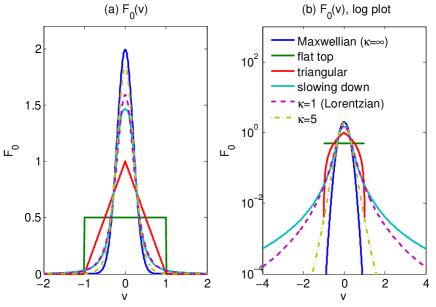
Figure 1: Typical distribution functions.

In this study, we investigate the analytical properties (particularly the singularity and analytic continuation problems) and develop a general numerical scheme for GPDF, i.e., for almost arbitrary input function $F$.

This problem was also discussed by RobinsonRobinson1990 , who used the linear combination of orthogonal functions. Three sets of orthogonal functions, Hermite, Legendre, and Chebyshev polynomials were discussed. Robinson’s method is very similar to our treatment in this study. However, he has neither given systematic results of the analytic continuation nor developed a one-solve-all scheme for practical application.

Our approach, which is discussed in Sec.II, is based on Hilbert transform (HT) and fast Fourier transform (FFT). After solving GPDF generally, we show several visualizations of GPDF in Sec.III. The distribution function effects on Landau damping are revisited in Sec.IV, and a summary and discussion are given in Sec.V.

II One-Solve-All Scheme for Generalized Plasma Dispersion Function

II.1 Hilbert transform and analytic continuation

HT is defined as

$$g(z)=H(f(z))=\frac{1}{\pi}\int_{-\infty}^{\infty}\frac{f(z^{\prime})}{z^{\prime}-z}dz^{\prime},$$ (10)

which can also be viewed as a convolution

$$g(z)=\frac{1}{\pi z}*f(z),$$ (11)

or the inverse

$$f(z)=-\frac{1}{\pi z}*g(z),$$ (12)

where $f(z)$ and $g(z)$ are called a Hilbert pair. HT usually represents a $90^{\circ}$ phase shift of input function.

Some useful properties include

1. $H(c_{1}f_{1}(z)+c_{2}f_{2}(z))=c_{1}g_{1}(z)+c_{2}g_{2}(z)$,

2. $H(H(f(z)))=-f(z)$,

3. $H(f(z+a))=g(z+a)$,

4. $H(f(az))=sgn(a)g(az)$,

5. $H(\frac{d^{n}f(z)}{dz^{n}})=\frac{d^{n}g(z)}{dz^{n}}$,

6. $f(z)+ig(z)$ is an analytical function.

A good scheme for numerically calculating HT in real line is provided by WeidemanWeideman1995 . Two other numerical methods are, using (10), i.e.,

$$g(z)\simeq\frac{2}{\pi}\sum_{n=-\infty}^{\infty}\frac{f(z+(2n+1)h)}{2n+1},$$ (13)

where $h$ is the step size, or using (11), i.e.,

$$g(z)=ift[ft(\frac{1}{\pi z})\cdot ft(f(z))],$$ (14)

where $ft()$ and $ift()$ denote the Fourier transform and its inverse.

The methods in Weideman’s 1995 paperWeideman1995 or via (13) and (14) are mainly for calculating integral principal value (PV) in real line.

In fact, the definition of (10) is not a single function. For simplification, we require $f(z)$ be an entire function that is integrable in the range of $-\infty$ to $+\infty$. The plasma dispersion function is defined for $\Im(z)>0$, and thus, should be extended to $\Im(z)\leq 0$, which isJones1985

$$g^{+}(z)=\left\{\begin{array}[]{ccc}\frac{1}{\pi}\int_{-\infty}^{\infty}\frac{f(z^{\prime})}{z^{\prime}-z}dz^{\prime},{}&\Im(z)>0,\\ \frac{1}{\pi}PV\int_{-\infty}^{\infty}\frac{f(z^{\prime})}{z^{\prime}-z}dz^{\prime}+if(z),{}&\Im(z)=0,\\ \frac{1}{\pi}\int_{-\infty}^{\infty}\frac{f(z^{\prime})}{z^{\prime}-z}dz^{\prime}+2if(z),{}&\Im(z)<0.\end{array}\right.$$ (15)

For instance, the HT of Lorentzian distribution $f(z)=\frac{a}{\pi}\frac{1}{z^{2}+a^{2}}$ is

$$g(z)=\left\{\begin{array}[]{ccc}-\frac{1}{\pi}\frac{1}{(z+ia)},{}&\Im(z)>0,\\ -\frac{z}{(z^{2}+a^{2})},{}&\Im(z)=0,\\ -\frac{1}{\pi}\frac{1}{(z-ia)},{}&\Im(z)<0,\end{array}\right.$$ (16)

whereas

$$g^{+}(z)=-\frac{1}{\pi}\frac{1}{(z+ia)},$$ (17)

which is consistent with (15).

$g^{-}(z)$ can be defined in a similar manner if we want to extend a function from lower half plane to the entire complex plane.

WeidemanWeideman1994 also provided a method to calculate $g^{+}(z)$ of the HT of Gaussian function in upper half plane, which is related to PDF $Z_{M}(\zeta)$.

II.2 One-solve-all approach

A comparison of (8) and (9) with (15) indicates $Z=\pi g^{+}$ and $Z_{p}=\pi g^{\prime+}$ with $F=f$ and $F^{\prime}=f^{\prime}$. Thus, GPDF is merely a HT of distribution function and shares the same properties of HT as listed in the above subsection.

Jones et al.Jones1985 also discussed the contour integral problem of GPDF and used transformation $z=tan(t)$ to map the integral of $z\in(-\infty,\infty)$ to $t\in(-\pi,\pi)$. This method is merely an alteration of (13) and requires other tricks to avoid singularity. Moreover, the method is time consuming and not suitable for high accuracy calculation as the discrete step should be very small to avoid divergence. Another direct numerical integral result is shown by Guio et al.Guio1998 with typical errors of $10^{-4}$.

In this paper, we use (15) to extend Weideman’s approachWeideman1994 ; Weideman1995 to the entire complex plane, where the orthogonal functions is $e^{i\theta}$, which can be evaluated very rapidly by FFT, instead of the Hermite, Legendre, and Chebyshev polynomials used by RobinsonRobinson1990 .

The key steps are summarized as follows.

Assuming an expansion

$$[W(v)]^{-1}F(v)=\sum_{n=-\infty}^{\infty}a_{n}\rho_{n}(v),~{}~{}~{}~{}v\in\mathcal{R}$$ (18)

where $\{\rho_{n}(v)\}$ is an orthogonal basis set with weight function $W(v)$, i.e.,

$$\int_{-\infty}^{\infty}W(v)\rho_{n}(v)\rho_{m}^{*}(v)dv=A\delta_{m,n},$$ (19)

where the asterisk denotes complex conjugation and $\delta_{m,n}$ is the Kronechker delta. The coefficients are

$$a_{n}=\frac{1}{A}\int_{-\infty}^{\infty}F(v)\rho_{n}^{*}(v)dv.$$ (20)

Then

$$\frac{F(v)}{v-z}=\sum_{n=-\infty}^{\infty}a_{n}\Big{[}W(v)\frac{\rho_{n}(v)}{v-z}\Big{]}.$$ (21)

For the upper half plane, we use weight function $W(v)=1/(L^{2}+v^{2})$Weideman1994 and basis functions

$$\rho_{n}(v)=\frac{(L+iv)^{n}}{(L-iv)^{n}},$$ (22)

which is a Fourier form because $e^{i\theta}=(L+iv)/(L-iv)$ with $v=L\tan(\theta/2)$ and $dv/d\theta=(L^{2}+v^{2})/(2L)$, then $a_{n}$ can be evaluated using FFT and we can obtain $A=\pi/L$ using $\int_{-\pi}^{\pi}e^{in\theta}e^{-im\theta}d\theta=2\pi\delta_{m,n}$.

Using residues, for $\Im(\zeta)>0$, we find the integrals

$$\int_{-\infty}^{\infty}\frac{W(v)}{v-z}\frac{(L+iv)^{n}}{(L-iv)^{n}}dv=\left\{\begin{array}[]{ccc}\frac{i\pi}{L}\frac{1}{(L-iz)},{}&n=0,\\ \frac{2i\pi}{L^{2}+z^{2}}\frac{(L+iz)^{n}}{(L-iz)^{n}},{}&n>0,\\ 0,{}&n<0.\end{array}\right.$$ (23)

We obtain

$$g^{+}(z)=\frac{2i}{L^{2}+z^{2}}\sum_{n=1}^{\infty}a_{n}\Big{(}\frac{L+iz}{L-iz}\Big{)}^{n}+\frac{ia_{0}}{L(L-iz)},~{}~{}~{}\Im(z)>0.$$ (24)

For the lower half plane, $\Im(\zeta)<0$, we use $F(z)=[F(z^{*})]^{*}$ and obtain

$$Z(\zeta)=[Z(\zeta^{*})]^{*}+2i\pi f(\zeta),~{}~{}~{}\Im(\zeta)<0.$$ (25)

For real line, $\Im(\zeta)=0$, we use $W(v)=1$ and $\rho_{n}(v)=(L+iv)^{n}/(L-iv)^{n+1}$Weideman1995 , and obtain

$$g^{+}(z) = \sum_{n=-\infty}^{\infty}isgn(n)a_{n}\rho_{n}(z)+if(z)$$ (26a)

$$= \sum_{n=0}^{\infty}2ia_{n}\rho_{n}(z),~{}~{}~{}\Im(z)=0.$$ (26b)

We have avoided the singularity on real line by treating the integrals of the basis functions analytically.

A completed scheme is provided through the combination of (24), (25) and (26), which can support an almost arbitrary smooth distribution function $F(v)$ and $F_{p}(v)=\partial F/\partial v$ as input function.

In numerical calculation, we truncate the summation at a finite point $n=N$. In the practical test for Gaussian input function with $N=32$, the program delivers twelve significant decimal digitsWeideman1994 , where $L$ is an optimal parameter and is set to $2^{-1/4}N^{1/2}$ as default.

Another good feature of this approach is that the coefficients $a_{n}$ need only be calculated once for all $z$, making the scheme even faster.

Moreover, an unexpected but interesting feature is that, the input function in the L.H.S. of (18) is not necessarily a smooth function. The R.H.S. of (18) can transform the real function $F(v)$ in real line to a smooth analytic complex function in whole complex plane with truncation. This feature can help us calculate several (note: not all) non-smooth input functions directly, such as flat top, incomplete Maxwellian, and slowing down. The validity of this approximation will be verified in Sec.III.

III Visualizations of Generalized Plasma Dispersion Function

III.1 Maxwellian distribution

First, we compare the results of the usual PDF with Maxwellian distribution as input function.

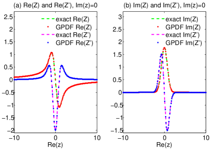
Figure 2: Comparison of our scheme for GPDF with exact $Z(\zeta)$ function via complex error function in standard numerical library on real axis.

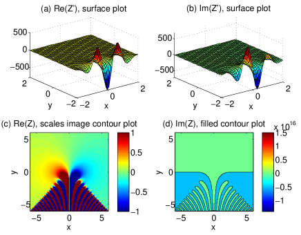
Figure 3: Visualization of $Z(\zeta)$ and $Z^{\prime}(\zeta)$ with Maxwellian input function.

Fig.2 shows a comparison of our scheme (using $N=32$) with exact $Z(\zeta)$ function via complex error function in standard numerical library on real axis. We find the errors to be around $10^{-12}$ (not shown in the figure), e.g., $Z(1)=-1.076159013825734+0.652049332173291i$ in our scheme and $Z(1)=-1.076159013825537+0.652049332173292i$ via standard library.

Fig.3 shows the 2D visualizations of $Z(\zeta)$ and $Z^{\prime}(\zeta)$ produced by our scheme, which shows that the functions are indeed analytically smooth. If we exclude the step for analytic continuation, we will find a jump at real line $\Im(z)=0$ (not shown here).

III.2 $\kappa$ distribution

With $F=\frac{1}{\pi(v^{2}+1)}$ as input function, a result is shown in Fig.4, where we can find a singularity at $z=-i$, which is consistent with analytical result (17).

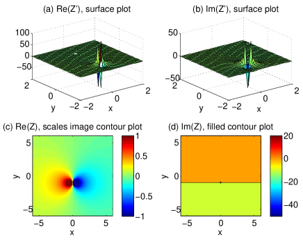
Figure 4: Visualization of $Z(\zeta)$ and $Z^{\prime}(\zeta)$ with input function $F=\frac{1}{\pi(v^{2}+1)}$, where artificial singular point NaN at $\zeta=i$ is kept.

However, another artificial singular point at $z=i$ [see panel (a)] can be found, where the code yields NaN. The two first-order singular points $v-ia=0$ and $v-z=0$ transformed into one second-order singular point $(v-ia)^{2}=0$ when $z=ia$ for Lorentzian input function. An extra approximation $Z(\zeta_{0})\simeq Z(\zeta_{0}+\epsilon)$ in the code is used to treat this kind of singular point, with $\zeta_{0}$ as the artificial singular point and $\epsilon$ be a small number, e.g., $10^{-10}$. After the extra treatment, we find GPDF yields exactly the same values as $\pi\times$(17) in all computation grids (not shown here) with controllable small errors.

After fixing this problem, a result is shown in Fig.5 for $\kappa=5$, $v_{t}=1$.

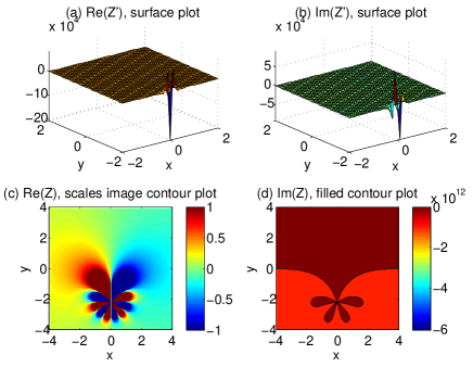
Figure 5: Visualization of $Z(\zeta)$ and $Z^{\prime}(\zeta)$ with input function $F_{\kappa=5}$.

To keep $\kappa=1$ the usual Lorentzian distribution, the definition of $\kappa$-distribution in (6) slightly differs from the usual oneSummers1991 but is close to the one by Valentini and D’AgostaValentini2007 .

III.3 $\delta$ distributions

The scheme described in Sec.II cannot support several non-standard distribution functions directly, particularly, $\delta$ distribution, which has been widely used for modeling cold plasma. We treat it separately in the code, via analytical expression.

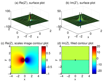
Figure 6: Visualizations of $Z(\zeta)$ with input function $F_{\delta}$ and parameters $z_{d}=0$.

For $\delta$-distribution $F_{\delta}=\delta(z-z_{d})$,

$$Z(\zeta) = -\frac{1}{\zeta-z_{d}},$$ (27a)

$$Z_{p}(\zeta) = \frac{1}{(\zeta-z_{d})^{2}},$$ (27b)

which can also be obtained from (17) using the limit $a\to 0$ because $\delta(v)=\lim\limits_{a\to 0}\frac{1}{\pi}\frac{a}{v^{2}+a^{2}}$. The result is shown in Fig.6.

III.4 Incomplete Maxwellian distributions

The input function is

$$F_{\text{IM}}(v)=H(v-\nu)\frac{1}{\sqrt{\pi}}e^{-v^{2}},$$ (28)

which has been investigated comprehensively by BaalrudBaalrud2013 , where $H$ is the Heaviside step function.

As previously mentioned, the numerical scheme cannot treat the $\delta$ function directly. For $Z^{\prime}$, an extra correction term should be added, i.e., $Z^{\prime}_{\text{IM}}(\zeta)=Z^{\prime}_{\text{IM0}}(\zeta)-\frac{1}{\sqrt{\pi}}e^{-\nu^{2}}/(\zeta-\nu)$, where $Z^{\prime}_{\text{IM0}}$ is the result without correction.

Figure 7: Visualization of $Z_{\text{IM}}(\zeta)$ and $Z^{\prime}_{\text{IM0}}(\zeta)$ with input function (28), where the absolute value and argument are calculated using $Z=|Z|e^{i\theta}$.

Fig.7 shows the results of $Z_{\text{IM}}(\zeta)$ and $Z^{\prime}_{\text{IM0}}(\zeta)$ calculated from our GPDF scheme, with $\nu=1$, $N=1024$ and $L=10$. Fig.7(a) is in favor of Fig.3(b) by BaalrudBaalrud2013 , which was calculated from a direct numerical integral. Our one-solve-all scheme can solve the same problem at least ten times faster than the direct numerical integral usually with the same accuracy.

A slight error can be found around the real line when $N$ is small, say $N=64$, which arises from the error of Fourier expansion around the sharp step place (Gibbs phenomenon) that requires a large $N$ to overcome.

III.5 Flat top distribution

For flat top distribution $F_{\text{Rect}}=\frac{H(z-z_{a})-H(z-z_{b})}{z_{b}-z_{a}}$,

$$Z(\zeta) = \frac{1}{z_{b}-z_{a}}\Big{[}\ln(\zeta-z_{b})-\ln(\zeta-z_{a})\Big{]},$$ (29a)

$$Z_{p}(\zeta) = \frac{1}{z_{b}-z_{a}}\Big{[}\frac{1}{\zeta-z_{b}}-\frac{1}{\zeta-z_{a}}\Big{]}.$$ (29b)

GPDF results and analytical results are compared in Fig.8. This benchmark indicates that our treatment for GPDF is indeed suitable for both smooth and non-smooth input function. However, to keep the result exactly the same as (29) at range $z_{a}\leq\zeta\leq z_{b}$ for lower half plane [$\Im(\zeta)<0$], the analytic continuation term $2if(z)$ is set to zero, instead of $2i/(z_{b}-z_{a})$.

For $Z^{\prime}_{\text{Rect}}$, we need also an extra treatment because of the $\delta$ function.

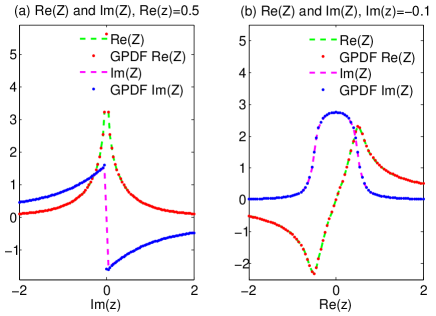
Figure 8: Comparison of GPDF results and analytical results for $Z(\zeta)$ with input function $F_{\text{Rect}}$ and parameters $z_{a}=-0.5$ and $z_{b}=0.5$.

III.6 Triangular distribution

The distribution function is

$$\begin{split}F_{\text{Tri}}&=\frac{H(z-z_{a})-H(z-z_{b})}{(z_{b}-z_{a})}\frac{2}{z_{c}-z_{a}}(z-z_{a})\\ &-\frac{H(z-z_{b})-H(z-z_{c})}{(z_{c}-z_{b})}\frac{2}{z_{c}-z_{a}}(z-z_{c}),\end{split}$$ (30)

and corresponding $Z(\zeta)$ is shown in Fig.9.

The analytic continuation term $2if(z)$ for lower half plane [$\Im(\zeta)<0$] is set to zero. Comparing root finding results and simulation results of Langmuir wave using the methods discussed in Sec.IV, we find that the solutions are the same (not shown here) for both cases, i.e., setting the term to zero or non-zero, and agreed with the simulations.

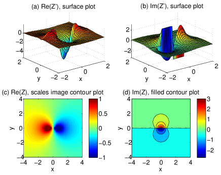
Figure 9: Visualization of $Z(\zeta)$ and $Z^{\prime}(\zeta)$ with input function $F_{\text{Tri}}$ and parameters $z_{a}=-1.0$, $z_{b}=0$ and $z_{c}=1$.

III.7 Slowing down distributions

The distribution function is very common in fusion plasma, such as tokamak, for fast particles,

$$F_{\text{SD}}=\frac{3\sqrt{3}v_{t}^{2}}{4\pi}\frac{1}{|v|^{3}+v_{t}^{3}}H(v_{c}-|v|).$$ (31)

A result is shown in Fig.10.

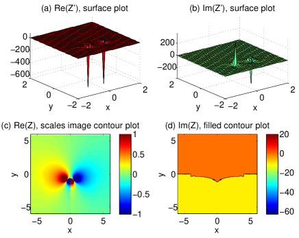
Figure 10: Visualization of $Z(\zeta)$ and $Z^{\prime}(\zeta)$ with input function $F_{\text{SD}}$ for $v_{t}=1$ and $v_{c}=4$.

One should note that the absolute value of $v$ in $F$ could cause problems in the complex plane, as $|\Re(v)+i\Im(v)|=\sqrt{\Re(v)^{2}+\Im(v)^{2}}\neq|\Re(v)|+i\Im(v)$. We use $H(v)$ to rewrite $|v|$ in the code, where $H(\Re(v)+i\Im(v))=H(\Re(v))[\Re(v)+i\Im(v)]$. Hence, we can still use $if(z)$ directly for the analytic continuation term to reduce numerical errors, instead of using the expansion expression $\sum a_{n}\rho_{n}$.

III.8 Other distributions

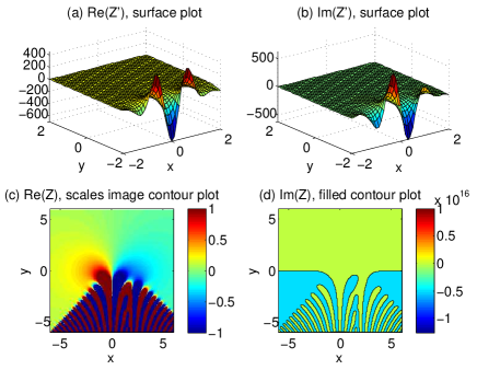
Figure 11: Visualization of $Z(\zeta)$ and $Z^{\prime}(\zeta)$ with bump-on-tail input function.

The GPDF has several good features such as for the bump-on-tail problem, when using usual PDF, the core plasma and beam plasma should to be treated separately. We can treat it using one input function directly when using GPDF. A result is shown in Fig.11 for $F=0.9e^{-v^{2}}/\sqrt{\pi}+0.1e^{-(v-2)^{2}}/\sqrt{\pi}$. A comparison with Fig.3 shows the beam tail affects $Z(\zeta)$ apparently, particularly at the place around $\Re(\zeta)=v_{d}=2$.

III.9 Short summary

The one-solve-all scheme has been shown to be effective. However, to treat non-smooth/analytical input functions, extra corrections should be noted. For non-smooth flat top and triangular distributions, the method of determining the analytic continuation requires further investigation, because it cannot be distinguished by Langmuir wave simulation.

From the visualizations of $Z(\zeta)$ and $Z^{\prime}(\zeta)$ for different types of input functions, the quantitative value, shape, or topology of $Z$ and $Z^{\prime}$ vary considerably, which will then bring different kinetic effects, e.g., Landau damping rate.

IV Distribution Function Effects on Landau Damping

IV.1 Benchmark GPDF using initial value scheme

For the initial value scheme, the starting equations are the normalized linear Vlasov-Poisson equations

$$\left\{\begin{aligned} {\partial_{t}\delta f}&=-ikv\delta f+\delta E{\partial_{v}{f_{0}}},\\ ik\delta E&=-\int{\delta fdv}.\end{aligned}\right.$$ (32)

We usually set $\lambda_{D}=1$, then $v_{t}=\sqrt{2}$ in the initial distribution function $f_{0}$, e.g., $f_{0}=\exp(-v^{2}/2)/\sqrt{2\pi}$ for Maxwellian.

Eqs.(32) can be solved as an initial value problem (IVP), e.g., using a 4th-order Runge-Kutta scheme, which should produce the exact linear Landau damping when the Case-Van Kampen mode and numerical errors are ignoredXie2013 . This simulation approach can be a simple and/or final benchmark for GPDF. Disagreements would mean the GPDF has been treated incorrectly. However, the IVP approach is not general, because of the numerical errors from discrete of $v$ and $t$, especially when the phase velocity $v_{p}=\omega/k$ or damping rate are large. A similar but more complicated IVP approach is used by Valentini and D’AgostaValentini2007 . Particle (e.g., particle-in-cell) simulation can also be used, which was also used by Godfrey et al.Godfrey1975 . Particle method can also easily support non-smooth distribution, but is limited by the noise resulting in unfavorable errors. Thus, this technique is not accurate when compared with the above continuum method.

Landau damping of Maxwellian distribution using this continuum IVP approach is verified in a previous workXie2013 .

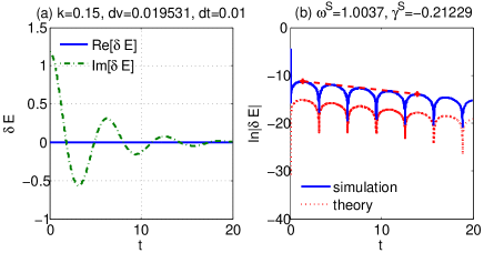
Figure 12: Benchmark GPDF using initial value simulation for Lorentzian distribution function. The result of root finding for this case is $\omega=1.0000-0.2121i$.

We check the Lorentzian distribution to show that our scheme for GPDF with non-Maxwellian distributions is also correct. Fig.12 shows the comparison of Lorentzian distribution Landau damping using IVP scheme and GPDF for $k=0.15$ and $v_{t}=\sqrt{2}$. We find that the simulation and numerical/analytical solutions match very well for both real frequency and damping rate, i.e., $\omega=1.00-0.212i$.

Another possible numerical approach for (32) is to treat it as an eigenvalue problem. However, the (Landau) damping normal mode is not eigenmode in this system, as discussed by numerous authors (see e.g., Xie2013 and references in). Thus, this approach does not work.

Notably, for GPDF, (5) would no longer be hold. Thus, $Z_{p}$ should be used for root finding instead of $Z$ to (4) or (1).

IV.2 Effects of discontinuity point

The $\delta$ function can be modeled as cold plasma, which provides the dispersion relation $(\omega-kv_{d})^{2}=\omega_{p}^{2}$. For discontinuity point such as the cases we meet in incomplete Maxwellian or flat top distributions, (29) can be used to solve the flat top case easily, which gives $(\omega-kv_{d})^{2}=\omega_{p}^{2}+k^{2}v_{t}^{2}$, where $v_{t}=(z_{b}-z_{a})/2$ and $v_{d}=(z_{b}+z_{a})/2$. The dispersion relation solutions of $\delta$ and flat top distributions are verified by PIC simulation (not shown here). For instance, for flat top distribution $v_{t}=1.0$, $v_{d}=0$, $k=1.0$, we obtain $\omega=1.414$, whereas PIC simulation yields $\omega_{r}\simeq 1.40$. For the continuum IVP simulation of discontinuity point, we use the approximation $\partial f_{0}/\partial v=[f_{0}(v_{0}^{+})-f_{0}(v_{0}^{-})]/\Delta v$, where $\Delta v$ is the velocity space grid size. In a practical test, the simulation also yields the same result, but is more accurate and has lower noise than PIC simulation. Thus, we use continuum IVP to verify GPDF results.

For incomplete Maxwellian distribution, we can compare the dispersion relation solutions of $Z^{\prime}_{\text{IM}}(\zeta)$ and $Z^{\prime}_{\text{IM0}}(\zeta)$ to investigate the effects of discontinuity point.

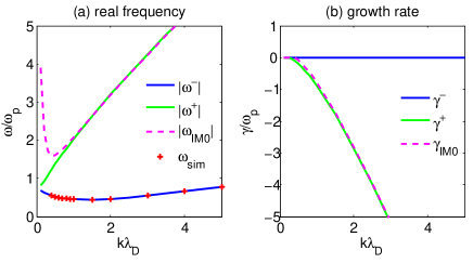
Figure 13: Dispersion relation solutions (root finding) of incomplete Maxwellian distribution with $\nu=-0.1v_{t}$, which agree with the simulation results very well.

The results are shown in Fig.13, with $\nu=-0.1v_{t}$ and $v_{t}=\sqrt{2}$. For example, $k=1.0$, $Z^{\prime}_{\text{IM}}$ yields $\omega^{+}=$2.0409-i0.8801 and $\omega^{-}=$-0.4542+i3.5173E-5; $Z^{\prime}_{\text{IM0}}$ yields $\omega=$2.0843-i0.7871, whereas IVP simulation yields $\omega\simeq$0.454+i0. Our solutions of $\omega^{\pm}$ via GPDF are in favor of the solutions by BaalrudBaalrud2013 . This benchmark provides further verification of the one-solve-all scheme.

Fig.13 shows that the discontinuity point at $v=\nu$ changes the dispersion properties considerably, for instance, a new nearly undamped branch can be found, which should be caused by the lack of resonance particles at $v_{p}=\omega/k<\nu$. The differences between the solutions of $Z^{\prime}_{\text{IM}}(\zeta)$ and $Z^{\prime}_{\text{IM0}}(\zeta)$ also indicates that an incorrect treatment of discontinuity point will yield inaccurate results.

IV.3 Results of distribution function effects

We use GPDF to revisit the distribution function effects on Landau damping.

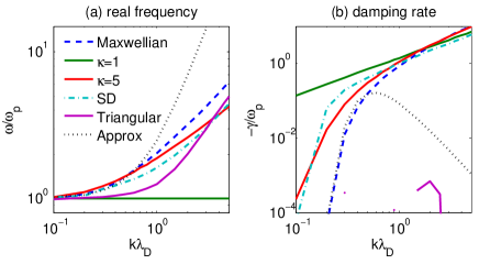
Figure 14: Distribution function effects on Landau damping with different initial distributions, where the approximate solution by (33) for Maxwellian distribution is also shown.

For Maxwellian distribution and small $k$, approximate analytical expressions for real frequency and growth rate areNicholson1983

$$\omega_{r}^{2}=\omega_{p}^{2}(1+3k^{2}\lambda_{D}^{2}),$$ (33a)

$$\omega_{i}=\frac{\pi}{2}\frac{\omega_{r}^{3}}{k^{2}}\frac{\partial f_{0}}{\partial v}\Big{|}_{v=\omega_{r}/k}.$$ (33b)

The effects of $\kappa$-distribution on Landau damping, particularly for space plasma, are discussed in detail by Thorne and SummersThorne1991 . The incomplete Maxwellian distribution is discussed by BaalrudBaalrud2013 .

Table 1: Comparison of the Langmuir wave solutions with different distribution functions and $k=1.0$.

-	$\omega_{r}^{G}$	$\omega_{i}^{G}$	$\omega_{r}^{S}$	$\omega_{i}^{S}$
Maxwellian	2.0459	-0.8513	2.01	-0.85
$\kappa=1$	1.0000	-1.4142	1.00	-1.40
$\kappa=5$	1.8786	-1.0866	1.82	-1.08
Slowing down	1.6240	-0.9975	$\simeq$1.68	$\simeq$-0.87
Triangular	1.2577	4.2E-4	$\simeq$1.26	$\simeq$0.005

We choose Maxwellian, $\kappa$, and slowing down distributions with $v_{t}=\sqrt{2}$ as well as triangular distributions with the same parameters as in Fig.9 for further comparisons. Fig.14 shows the results of $\omega_{r}$ vs. $k$ and $\gamma$ vs. $k$. For triangular distribution, a non-zero $\gamma$ around $\pm 10^{-4}$ exists but is sensitive to initial guessing for the root finding, which should be caused by the jump of $Z^{\prime}$ around $\Im(z)=0$ as shown in Fig.9.

Table 1 shows the quantitative value of the solutions, where $\omega^{G}$ is solved from GPDF and $\omega^{S}$ is from IVP simulation. For non-smooth input distributions, the simulation is not robust and is sensitive to parameters and initial conditions. Several results in table ($k=1.0$) are very rough (labeled with ‘$\simeq$’). For instance, the error of the result in this table for slowing down distribution is very large (approximately $10\%$), whereas, for small $k$ and small damping rate, e.g., $k=0.5$, IVP simulation is more robust and accurate, and we obtain $\omega^{S}_{SD}=1.29-0.42i$ compared with $\omega^{G}_{SD}=1.2876-0.4119i$.

V Summary and Discussion

The analytical properties and one-solve-all numerical scheme for generalized plasma dispersion function, which provides a useful tool for treating linear effects of almost arbitrary distribution functions, are discussed. The exact distribution function effects on Landau damping are revisited to demonstrate an application.

The one-solve-all scheme can also be used analytically as an expansion method for GPDF, in addition to the usual Taylor expansion scheme used.

Our method cannot be used directly for relativisticGodfrey1975 ; Castejon2006 or other more complicated dispersion functions because those dispersion functions are usually not in HT form. However, similar orthogonal functions expansion treatment may be used, as mentioned by RobinsonRobinson1990 .

VI Acknowledgements

Discussions with Y. R. Lin-Liu at the early stage of this project to understand the treatment of usual PDF are appreciated. This work is support by the NSF of China under Grants No.11235009, the ITER-CN under Grant No. 2013GB104004 and Fundamental Research Fund for Chinese Central Universities.

References

- (1) D. R. Nicholson, Introduction to Plasma Theory (Wiley, 1983).
- (2) B. D. Fried and S. D. Conte, The Plasma Dispersion Function THE HILBERT TRANSFORM OF THE GAUSSIAN (Academic Press, New York and London, 1961). Erratum: Math. Comp. v. 26, 1972, no. 119, p. 814. Reviews and Descriptions of Tables and Books, Math. Comp., v. 17, 1963, pp. 94-95.
- (3) F. Valentini and R. D’Agosta, Phys. Plasmas 14, 092111 (2007).
- (4) D. Summers and R. M. Thorne, Phys. Fluids B 3, 1835 (1991).
- (5) S. D. Baalrud, Phys. Plasmas 20, 012118 (2013).
- (6) M. A. Hellberg and R. L. Mace, Phys. Plasmas 9, 1495 (2002).
- (7) P. A. Robinson, Journal of Computational Physics 88, 381 (1990).
- (8) J. A. C. Weideman, Mathematics of Computation 64, 745 (1995).
- (9) J. A. C. Weideman, SIAM J. Numer. Anal. 31, 1497 (1994).
- (10) W. D. Jones, H. J. Doucet and J. M. Buzzi, An Introduction to the Linear Theories and Methods of Electrostatic Waves in Plasmas (Springer, 1985).
- (11) P. Guio, J. Lilensten, W. Kofman and N. Bjorna, Annales Geophysicae 16, 1226 (1998).
- (12) H. S. Xie, Constant residual electrostatic electron plasma mode in Vlasov-Ampere system, submitted to Phys. Plasmas.
- (13) R. M. Thorne and D. Summers, Phys. Fluids B 3, 2117 (1991).
- (14) B. B. Godfrey, B. S. Newberger and K. A. Taggart, IEEE Transactions on Plasma Science 3, 60 (1975).
- (15) F. Castejon and S. S. Pavlov, Phys. Plasmas 13, 072105 (2006).