Flavour structure of the nucleon electromagnetic form factors and transverse charge densities in the chiral quark-soliton model

Abstract

We investigate the flavour decomposition of the electromagnetic form factors of the nucleon, based on the chiral quark-soliton model ($\chi$QSM) with symmetry-conserving quantisation. We consider the rotational $1/N_{c}$ and linear strange-quark mass ($m_{s}$) corrections. We discuss the results of the flavour-decomposed electromagnetic form factors in comparison with the recent experimental data. In order to see the effects of the strange quark, we compare the SU(3) results with those of SU(2). We finally discuss the transverse charge densities for both unpolarised and polarised nucleons. The transverse charge density inside a neutron turns out to be negative in the vicinity of the centre within the SU(3) $\chi$QSM, which can be explained by the contribution of the strange quark.

I Introduction

Electromagnetic form factors (EMFFs) are the most fundamental observables that reveal the charge and magnetisation structures of the nucleon. A series of recent measurements of the EMFFs has renewed the understanding of the internal structure of the nucleon and has posed fundamental questions about its nonperturbative nature. The results of the ratio of the proton EMFFs, $\mu_{p}G_{E}^{p}/G_{M}^{p}$ with the proton magnetic moment $\mu_{p}$, obtained by measuring the transverse and longitudinal recoil proton polarisations Jones:1999rz ; Gayou:2001qt ; Gayou:2001qd ; Punjabi:2005wq ; Puckett:2010ac ; Bernauer:2010wm ; Ron:2011rd ; Zhan:2011ji , were found to decrease almost linearly with $Q^{2}$ above $1\,(\mathrm{GeV}/c)^{2}$. These results were in conflict with most of the previous measurements of the proton EMFFs from unpolarised electron-proton cross sections based on the Rosenbluth separation method.These new experimental results have triggered subsequent theoretical and experimental works (see, for example, recent reviews HydeWright:2004gh ; Arrington:2006zm ; Perdrisat:2006hj ; Vanderhaeghen:2010nd ; Arrington:2011kb ). This discrepancy is partially explained by the effects of two-photon exchange, which affect unpolarised electron-proton scattering at higher $Q^{2}$ but have less influence on the polarisation measurements Guichon:2003qm ; Blunden:2003sp ; Arrington:2004ae ; Arrington:2007ux ; Carlson:2007sp ; Arrington:2011dn . Moreover, the new experimental results of the proton EMFFs in a wider range of $Q^{2}$ provided a whole new perspective on the internal quark-gluon structure of the nucleon. Perturbative quantum chromodynamics (pQCD) with factorisation schemes Brodsky:1974vy predicts the different scalings of the Dirac and Pauli FFs, $F_{1}^{p}$ and $F_{2}^{p}$: $F_{1}^{p}$ falls off as $1/Q^{4}$ while $F_{2}^{p}$ decreases as $1/Q^{6}$, so that $Q^{2}F_{2}^{p}/F_{1}^{p}$ becomes flat at large $Q^{2}$. However, the experimental data show that the ratio $Q^{2}F_{2}^{p}/F_{1}^{p}$ increases with $Q^{2}$ but $QF_{2}^{p}/F_{1}^{p}$ becomes flat starting around $2\,\mathrm{GeV}^{2}$. A similar discrepancy between the experimental data and pQCD was also found in the $\gamma\gamma^{*}\to\pi$ transition form factor Aubert:2009mc ; Uehara:2012ag even for higher $Q^{2}$. It implies that it is far more important to consider effects from nonperturbative physics than those from perturbative QCD in lower $Q^{2}$ region.

Assuming isospin and charge symmetries, neglecting the strangeness in the nucleon, and using both the experimental data for the proton and neutron EMFFs, Cates et al. Cates:2011pz have extracted the up and down EMFFs and have obtained remarkable results: the $Q^{2}$ dependence of the up- and down-quark Dirac ($F_{1}$) and Pauli ($F_{2}$) form factors (FFs) are considerably different from each other. The down-quark Dirac and Pauli FFs are roughly proportional to $1/Q^{4}$ but those of the up-quark fall off more gradually. Moreover, while the ratios $\kappa_{u}^{-1}F_{2}^{u}/F_{1}^{u}$ and $\kappa_{d}^{-1}F_{2}^{d}/F_{1}^{d}$ ($\kappa$ is the anomalous magnetic moment) are relatively constant above $Q^{2}\sim 1\,\mathrm{GeV}^{2}$, they show a complicated behavior for lower $Q^{2}$ regions. Qattan and Arrington Qattan:2012zf ; Qattan:2015qxa elaborated on the analysis of Ref. Cates:2011pz , taking into account explicitly the effects of two-photon exchange and uncertainties on the proton form factor and the neutron magnetic FFs. They found that the ratio of the up-quark EMFFs ($G_{E}^{u}/G_{M}^{u}$) has a roughly linear drop-off, while that of the down-quark EMFFs ($G_{E}^{d}/G_{M}^{d}$) showed a completely different dependence on $Q^{2}$. As a result, the flavour-decomposed FFs behave in a different way from the proton EMFFs. Diehl and Kroll Diehl:2013xca critically analyzed experimental data in order to study several hadron properties and also obtained a separation of the light quark contributions to form factors. The flavour contributions to the EMFFs of the nucleon and the related charge and magnetization densities had already been the subject of interest prior to the phenomenological analysis of Cates:2011pz and of Qattan:2012zf ; Diehl:2013xca : Ref. Cloet:2008re used a framework based on the Faddeev equation with dressed quarks to obtain the flavor contributions to the Dirac, Pauli and Sachs form factors, including the associated radii, while Crawford:2010gv used a vector dominance model. These studies, as well as experimental results Riordan:2010id , pointed out the nontrivial behaviour of these contributions as revealed further by the analysis of Cates:2011pz ; Qattan:2012zf ; Diehl:2013xca . Several theoretical studies of these contributions have since been performed: Ref. Eichmann:2011vu further developed the covariant Faddeev framework, based on the Dyson-Schwinger equations of QCD,  Rohrmoser:2011tw ; Rohrmoser:2017zpk employed a Goldstone-boson-exchange relativistic constituent quark model,  Cloet:2012cy extended the quark-diquark model to include a pion cloud. In Ref. GonzalezHernandez:2012jv the flavour contributions to the EMFFs were obtained by computing the generalized parton distributions in a reggeized diquark model and in Chakrabarti:2013dda from generalized parton distributions obtained in a quark model in AdS/QCD. The AdS/QCD correspondence has been the basis for similar studies within different approaches: in a light-front quark model in a soft-wall model Mondal:2015uha ; or a hard-wall model Mondal:2016xpk ; also via parameterization approaches, Sharma:2016cnf and Nikkhoo:2015jzi . Ref. Brodsky:2016uln used the light-front holographic QCD framework including higher Fock components and Ref. Obukhovsky:2014xja a relativistic light-front model. The flavour contributions may equally be displayed through the transverse charge and magnetization densities, as one may find in Ref.s Chakrabarti:2014dna ; Sharma:2014voa , which employed a soft-wall model of AdS/QCD, and also in some of the aforementioned studies.

In this context, we investigated the flavour structure of the nucleon EMFFs within the framework of the self-consistent SU(2) and SU(3) chiral quark-soliton models ($\chi$QSMs) Diakonov:1987ty ; Wakamatsu:1990ud ; Blotz:1992pw . The $\chi$QSM has described successfully various observables of the baryon octet and decuplet (For reviews, see Alkofer:1994ph ; Christov:1995vm ; Weigel:2008zz ; Goeke:2001tz ). In particular, the $Q^{2}$ dependence of almost all form factors is well reproduced within the $\chi$QSM, so that the strange-quark EMFFs Goeke:2006gi and the parity-violating (PV) asymmetries of polarised electron-proton scattering Silva:2005qm , which require nine different FFs (six EMFFs and three axial-vector FFs) with the same set of parameters, are in good agreement with experimental data. Thus, it is worthwhile to examine the flavour structure of the nucleon EMFFs in detail. As mentioned, the nucleon EMFFs were already studied in the SU(3) $\chi$QSM Kim:1995mr . However, Praszałowicz et al. Praszalowicz:1998jm pointed out that the Gell-Mann-Nishijima relation was not exactly fulfilled in the initial version of the $\chi$QSM and proposed the symmetry-conserving quantisation that makes the Gell-Mann-Nishijima relation well satisfied. We want to emphasize that the $\chi$QSM is a reasonable framework to investigate properties of the lowest-lying SU(3) baryons. Witten originally proposed in his seminal papers Witten:1979kh ; Witten:1983 that the lowest-lying light baryons may be regarded as bound states of $N_{c}$ valence quarks in a meson mean field. In the limit of the large number of colours ($N_{c}$), the lowest-lying SU(3) baryons constitute $N_{c}$ valence quarks that bring about an effective pion mean field or the vacuum polarization. The value of $N_{c}$ will be taken to be three at the final stage of the computation such that we are able to compare the present results with the experimental data. Recently, this mean-field approach or the $\chi$QSM described successfully properties of singly heavy baryons Yang:2016qdz ; Kim:2017jpx ; Kim:2017khv .

In this work, we present the results of the flavour-decomposed up- and down-quark EMFFs based on the SU(3) $\chi$QSM with symmetry-conserving quantisation employed. We first show the Dirac and Pauli FFs of the nucleon and then examine the $Q^{2}$ dependence of the up- and down-quark Dirac and Pauli FFs. The ratio of the flavour-decomposed Dirac and Pauli FFs will be discussed, compared with the recent experimental data Qattan:2012zf . We also reexamine the results of the strange EMFFs, since there are new experimental data from PV polarised electron-nucleon scattering. In particular, the G0 collaboration recently measured the paritiy-violating asymmetries in the backward angle Androic:2009aa , which was first predicted in Ref. Silva:2005qm . In addition to the flavour decomposed EMFFs of the nucleon, we also investigate the charge and magnetisation densities of the quark in a nucleon in the transverse plane. Together with the new experimental data for the nucleon EMFFs, the nucleon GPDs cast light on the concept of nucleon FFs Ji:1998pc ; Goeke:2001tz ; Diehl:2003ny ; Belitsky:2005qn .

The present work is sketched as follows. In Section 2, we briefly review the general formalism of the EMFFs of the nucleon and its flavour decomposition and describe how to compute the EMFFs of the nucleon within the framework of the SU(2) and SU(3) $\chi$QSMs. In the following sections we present the results and discuss their physical implications in the light of the recent experimental data: for Sachs FFs in Section 3 and for the Dirac and Pauli FFs in Section 4. In section 5 we also present the model results for the transverse charge and magnetic distributions of the quark inside both unpolarised and transversely polarised nucleons. The final Section is devoted to the summary and the conclusions.

II Electromagnetic Form factors and the $\chi$QSM

The matrix element of a flavour vector current between the two nucleon states is expressed in terms of the flavour Dirac and Pauli FFs

$$\langle N(p^{\prime},\,s^{\prime})|J_{\mu}^{\chi}(0)|N(p,\,s)\rangle$$ (2)

$$=\bar{u}_{N}(p^{\prime},\,s^{\prime})\left[\gamma_{\mu}F_{1}^{\chi}(q^{2})+i\sigma_{\mu\nu}\frac{q^{\nu}}{2M_{N}}F_{2}^{\chi}(q^{2})\right]u_{N}(p,\,s),$$

where $J_{\mu}^{\chi}(0)$ represents the flavour vector current defined as

$$J_{\mu}^{\chi}(0)\;=\;\bar{\psi}(0)\lambda^{\chi}\gamma_{\mu}\psi(0).$$ (3)

$\chi$ denotes the flavour index, i.e. $\chi=0,\,3,\,8$ for the flavour decomposition. Here, one has to bear in mind that $\lambda^{0}$ is considered to be a unity flavour matrix. Thus, the normalisation $\{\lambda^{a},\,\lambda^{b}\}=2\delta^{ab}$ for $\lambda^{\chi}$ applies only to the Gell-Mann matrices with $\chi=3$ and $\chi=8$. The Dirac spinor $u_{N}(p,\,s)$ applies to the nucleon with mass $M_{N}$, momentum $p$ and the third component of its spin $s$. The square of the four momentum transfer is denoted by $q^{2}=-Q^{2}$, with $Q^{2}>0$. The flavour Dirac and Pauli FFs can be combined to give the Sachs FFs:

$$G^{\chi}_{E}(Q^{2}) = F_{1}^{\chi}(Q^{2})-\frac{Q^{2}}{4M^{2}_{N}}F_{2}^{\chi}(Q^{2})$$

$$G_{M}^{\chi}(Q^{2}) = F_{1}^{N}(Q^{2})+F_{2}^{\chi}(Q^{2}).$$ (4)

In the Breit frame, $G_{E}^{\chi}(Q^{2})$ and $G_{M}^{\chi}(Q^{2})$ are related to the time and space components of the flavour vector current, respectively:

$$G^{\chi}_{E}(Q^{2}) = \langle N^{\prime}(p^{\prime})|\bar{\psi}(0)\gamma_{0}\lambda^{\chi}\psi(0)|N(p)\rangle$$

$$G^{\chi}_{M}(Q^{2}) = iM_{N}\epsilon_{ilk}\frac{q_{l}}{6q^{2}}{\rm tr}\left(\langle p^{\prime},\lambda^{\prime}|\bar{\psi}(0)\gamma_{i}\lambda^{\chi}\psi(0)|p,\lambda\rangle\sigma_{k}\right).$$ (5)

where $\sigma_{j}$ are the Pauli spin matrices. The $|\lambda\rangle$ is the corresponding spin state of the nucleon.

In SU(3) flavour the nucleon EMFFs are expressed in terms of the triplet and octet vector form factors

$$G_{E,M}^{N}(Q^{2})\;=\;\frac{1}{2}\left(G_{E,M}^{3}+\frac{1}{\sqrt{3}}G_{E,M}^{8}\right),$$ (6)

while in flavour SU(2) they are written as

$$G_{E,M}^{N}(Q^{2})\;=\;\frac{1}{2}\left(\frac{1}{3}G_{E,M}^{0}+G_{E,M}^{3}\right).$$ (7)

Although the same notation is used for the form factors, it will always follow from the context which flavour case is being addressed.

The matrix elements given in Eq. (5) can be evaluated both in the SU(2) and SU(3) flavour $\chi$QSMs. The model starts from the following low-energy effective partition function in Euclidean space

$$\mathcal{Z}_{\mathrm{\chi QSM}} = \int\mathcal{D}\psi\mathcal{D}\psi^{\dagger}\mathcal{D}U\exp\left[-\int d^{4}x\Psi^{\dagger}iD(U)\Psi\right]$$ (8)

$$= \int\mathcal{D}U\exp(-S_{\mathrm{eff}}[U])\,,$$ (9)

where $\psi$ and $U$ denote the quark and pseudo-Goldstone boson fields, respectively. After integrating over the quark fields, the effective chiral action $S_{\mathrm{eff}}$ is given by

$$S_{\mathrm{eff}}(U)\;=\;-N_{c}\mathrm{Tr}\ln iD(U)\,,$$ (10)

where $\mathrm{Tr}$ represents the functional trace and $N_{c}$ the number of colours.

The Dirac $D(U)=\gamma_{4}(i\hbox to0.0pt{/\hss}{\partial}-\hat{m}-MU^{\gamma_{5}})$ operator, depending on the flavour space, is given by

$$D_{\mathrm{SU(2)}}(U) = -i\partial_{4}+h(U)$$ (11)

$$D_{\rm SU(3)}(U) = -i\partial_{4}+h(U)-\gamma_{4}\delta m$$ (12)

since, as isospin symmetry is assumed in this work, $\hat{m}=\mathrm{diag}(\overline{m},\,\overline{m})=\overline{m}\mathbf{1}_{2}$ in SU(2) and $\hat{m}=\mathrm{diag}(\overline{m},\,\overline{m},\,m_{\mathrm{s}})=\overline{m}\mathbf{1}_{3}+\delta m$ in SU(3), where

$$\delta m\;=\;\frac{-\overline{m}+m_{s}}{3}\mathbf{1}_{3}+\frac{\overline{m}-m_{s}}{\sqrt{3}}\lambda^{8}=M_{1}\mathbf{1}_{3}+M_{8}\lambda^{8}\,.$$ (13)

The mass term $\delta m$ containing the strange current quark mass $m_{s}$ will be treated as a perturbation.

The single-quark Hamiltonian $h(U)$ is expressed as

$$h(U)\;=\;i\gamma_{4}\gamma_{i}\partial_{i}-\gamma_{4}MU^{\gamma_{5}}-\gamma_{4}\overline{m}\,,$$ (14)

where $U^{\gamma_{5}}$ stands for the chiral field for which we assume Witten’s embedding of the SU(2) soliton into SU(3)

$$U^{\gamma_{5}}_{\mathrm{SU(3)}}\;=\;\left(\begin{array}[]{lr}U_{\mathrm{SU(2)}}^{\gamma_{5}}&0\\ 0&1\end{array}\right)$$ (15)

with the SU(2) pion field $\pi^{i}$ as

$$U_{\mathrm{SU(2)}}^{\gamma_{5}}\;=\;\exp(i\gamma^{5}\tau^{i}\pi^{i})\;=\;\frac{1+\gamma^{5}}{2}U_{\mathrm{SU(2)}}+\frac{1-\gamma^{5}}{2}U_{\mathrm{SU(2)}}^{\dagger}.$$ (16)

The integration over the pion field $U$ in Eq. (9) can be performed by the saddle-point approximation in the large $N_{c}$ limit due to the $N_{c}$ factor in Eq. (10). The SU(2) pion field $U$ is written as the most symmetric hedgehog form

$$U_{\mathrm{SU(2)}}\;=\;\exp[i\gamma_{5}\hat{\bm{n}}\cdot{\bm{\tau}}P(r)]\,,$$ (17)

where $P(r)$ is the radial profile function of the soliton.

The $\chi$QSM nucleon state $|N(p,\,s)\rangle$ used in the computation of Eqs. (2) and (5) is defined in terms of an Ioffe-type current consisting of $N_{c}$ quarks:

$$|N(p,\,s)\rangle\;=\;\lim_{x_{4}\rightarrow-\infty}\,\frac{1}{\sqrt{\mathcal{Z}}}\,e^{ip_{4}x_{4}}\,\int d^{3}{\bm{x}}\,e^{i\,{\bm{p}}\cdot{\bm{x}}}\,J_{N}^{\dagger}(x)\,|0\rangle$$ (18)

with the Ioffe-type nucleon current $J_{N}$ defined as

$$J_{N}(x)\;=\;\frac{1}{N_{c}!}\,\Gamma_{N}^{b_{1}\cdots b_{N_{c}}}\,\varepsilon^{\beta_{1}\cdots\beta_{N_{c}}}\,\psi_{\beta_{1}b_{1}}(x)\cdots\psi_{\beta_{N_{c}}b_{N_{c}}}(x)\,.$$ (19)

Here, the matrix $\Gamma_{N}^{b_{1}...b_{N_{c}}}$ carries the hypercharge $Y$, isospin $I,I_{3}$ and spin $s,s_{3}$ quantum numbers of the baryon and the $b_{i}$ and $\beta_{i}$ denote the spin-flavour and colour indices, respectively.

After minimizing the action in Eq. (10), we derive an equation of motion which is solved self-consistently with respect to the function $P(r)$ in Eq. (17). The corresponding unique solution $U_{c}$ is called the classical chiral soliton. The next step consists in quantising the classical soliton. This can be achieved by quantising the rotational and translational zero-modes of the soliton. The rotations and translations of the soliton are implemented by

$$U({\bm{x}},t)=A(t)U_{c}({\bm{x}}-{\bm{z}}(t))A^{\dagger}(t)\,,$$ (20)

where $A(t)$ denotes a time-dependent SU(3) matrix, related to the orientation of the soliton in coordinate and flavour spaces, and ${\bm{z}}(t)$ stands for the time-dependent translation of the centre of mass of the soliton in coordinate space. The rotational velocity of the soliton $\Omega(t)$ is defined as

$$\Omega=\frac{1}{i}A^{\dagger}\dot{A}=\frac{1}{2i}\textrm{Tr}(A^{\dagger}\dot{A}\lambda^{\alpha})\lambda^{\alpha}=\frac{1}{2}\Omega_{\alpha}\lambda^{\alpha}.$$ (21)

Treating $\Omega(t)$ and $\delta m$ perturbatively with slowly rotating soliton and small $\delta m$ considered, we find the collective Hamiltonian, i.e, the Hamiltonian in the collective coordinates of position of the centre of mass and the orientation of the soliton, which is given explicitly as

$$H_{\mathrm{coll}}^{\mathrm{SU(2)}}=M_{c}^{\mathrm{SU(2)}}+\frac{1}{2I_{1}^{\mbox{\tiny SU(2)}}}\sum_{i=1}^{3}J_{i}J_{i}$$ (22)

in SU(2) and as

$$H_{\mathrm{coll}}^{\mathrm{SU(3)}} = H_{\mathrm{sym}}+H_{\mathrm{sb}}$$ (23)

$$H_{\mathrm{sym}} = M_{c}+\frac{1}{2I_{1}}\sum_{i=1}^{3}J_{i}J_{i}+\frac{1}{2I_{2}}\sum_{a=4}^{7}J_{a}J_{a},$$ (24)

$$H_{\mathrm{sb}} = \frac{1}{\overline{m}}M_{1}\Sigma_{SU(2)}+\alpha D_{88}^{(8)}(A)+\beta Y+\frac{\gamma}{\sqrt{3}}D_{8i}^{(8)}(A)J_{i}\,.$$ (25)

in SU(3). The $M_{c}$ is the classical mass of the state, the parameters $I$ are inertia parameters, $Y$ is the hypercharge, $\Sigma_{SU(2)}$ is the pion-nucleon sigma term, the $J$s are the angular momentum operators and $D^{(8)}$ are the SU(3) Wigner $D$ functions. It is obvious that the strange quark in flavour SU(3) leads to a more involved analysis, particularly to the symmetry breaking contributions.

Within the collective quantisation procedure the nucleon states given in Eq. (18) will be mapped to collective rotational functions carrying the state quantum numbers. In flavour SU(2) these functions are the eigenfunctions of the SU(2) symmetrical Hamiltonian, i.e., the Wigner $D$ functions given as

$$\Psi_{JJ_{3}TT_{3}}(A) = \langle A|N(JJ_{3};\,TT_{3})\rangle$$ (26)

$$= (-1)^{T+T_{3}}\sqrt{2T+1}D^{T=J}_{-T_{3},J_{3}}(A).$$ (27)

In flavour SU(3) the eigenfunctions of the SU(3) symmetric part of the Hamiltonian turn out to be the SU(3) Wigner $D$ functions

$$\Psi^{n}_{Y;JJ_{3};TT_{3}}(A) = \langle A|N(Y;\,JJ_{3};\,TT_{3})\rangle$$ (28)

$$= \sqrt{\dim n}(-1)^{-1/2+J_{3}}D^{(n)*}_{T,T_{3},Y;J,J_{3},-1}(A).$$ (29)

On the contrary to the SU(2) case, the nucleon state is no longer a pure octet state but is a mixed state with those in higher representations arising from flavour SU(3) symmetry breaking, i.e.

$$|N(Y;JJ_{3};TT_{3})\rangle\;=\;|8_{1/2}\>(Y;JJ_{3};TT_{3})\rangle$$ (31)

$$+c_{\overline{10}}\sqrt{5}|\overline{10}_{1/2}\>(Y;JJ_{3};TT_{3})\rangle+c_{27}\sqrt{6}|27_{1/2}\>(Y;JJ_{3};TT_{3})\rangle,$$

where $c_{\overline{10}}$ and $c_{27}$ denote the mixing parameters. These parameters, as well as the $\alpha$, $\beta$ and $\gamma$ in Eq. (25), may be found in Refs. Blotz:1992pw ; Christov:1995vm .

A detailed formalism for the zero-mode quantisation can be found in Refs. Blotz:1992pw ; Christov:1995vm . In addiction, Ref. Kim:1995mr offers a detailed description as to how the form factors can be obtained numerically. We briefly summarise it here before we discuss the numerical results. The parameters existing in the model are the constituent quark mass $M$, the current quark mass $\overline{m}$, the strange current quark mass $m_{\mathrm{s}}$, and the cutoff mass $\Lambda$ of the proper-time regularisation. However, not all of them are free parameters but can be fixed in the mesonic sector without any ambiguity. In fact, this is a merit of the $\chi$QSM in which mesons and baryons can be treated on an equal footing. For a given $M$ the regularisation cut-off parameter $\Lambda$ and the current quark mass $\overline{m}$ in the Lagrangian are fixed to the pion decay constant $f_{\pi}=93$ MeV and the physical pion mass $m_{\pi}=140$  MeV, respectively. The strange current quark mass is taken to be $m_{\mathrm{s}}=180\,\textrm{MeV}$ which approximately reproduces the kaon mass. Though the constituent quark mass $M$ can be regarded as a free parameter, it is also more or less fixed. The experimental proton electric charge radius is best reproduced in the $\chi$QSM with the constituent quark mass $M=420$ MeV. Moreover, the value of 420 MeV is known to yield the best fit to many baryonic observables Christov:1995vm . Thus, all the numerical results in the present work are obtained with this value of $M$.

All the results presented in the following were computed completely within the model, in the same level of approximation, to keep consistency. In particular, magnetisation observables are presented not in terms of the physical nuclear magneton but, instead, in terms of the model nuclear magneton, i.e. defined as the model value for the nucleon mass, which, at this level of approximation used in this work, is

$$M_{N}=1250\;\textrm{MeV}.$$ (32)

We want to mention that the ratio between the model nuclear magneton and the physical one is the same as that between the value of $M_{N}$ in Eq.(32) and the physical nucleon mass.

To address the properties of the baryon octet implies immediately flavour structures of the SU(3) baryons. However, it indicates simultaneously the question as to how accurate is the $\chi$QSM description of the strangeness content of the nucleon and its implications to the EMFF. Such a question could easily be answered if one had precise experimental data on the strange EMFF. The present study may give some clues to the answer for that question in the light of the recent phenomenological data Cates:2011pz ; Qattan:2012zf .

III Sachs form factors

The Sachs EM form factors Ernst:1960zza ; Sachs:1962zzc are the most common form to encompass information about the electromagnetic structure of the nucleon. On the one hand, these form factors make it possible to express the cross section for elastic electron-proton scattering in the one-photon exchange approximation, without mixed terms ($G_{E}G_{M}$) in a form suitable for the separation of the electric and magnetic form factors. That is not the case when the cross section is expressed in terms of the Dirac and Pauli form factors (2), where the mixed terms ($F_{1}F_{2}$) occur. Even with the more recent polarisation transfer methods Arnold:1980zj , the measured ratio between the longitudinal and transverse polarisation components is expressed in terms of the Sachs form factors ratio $\mu G_{E}/G_{M}$.

On the other hand, the Sachs form factors have a merit that in the Breit frame they may be apparently interpreted as the Fourier transform of the charge and magnetisation distributions inside a nucleon. It comes from the fact that in the Breit frame the proton does not exchange energy with the virtual photon with momentum $(0,\,{\bm{q}})$. At a specific space-like $Q^{2}=-{\bm{q}}^{2}<0$ invariant momentum transfer, the time and space components of the electromagnetic current, associated with the electric and magnetic form factors respectively, resemble the classical non-relativistic current density. Hence the Sachs EM form factors are directly related to the charge and magnetisation distributions by the Fourier transform. However, these relations are supposedly non-relativistic in nature due to the $Q^{2}$ dependence of the Breit-frame. Both the preceding features of the Sachs form factors are currently under scrutiny, as mentioned in Introduction. Discrepancies in the experimental results from the elastic $ep$ cross section and polarisation transfer studies called for the inclusion of new aspects of elastic electron proton scattering, such as the two-photon exchange Carlson:2007sp . The connection between form factors and densities, even apart from the non-relativistic limitation, has also been revised on general grounds Miller:2007uy ; Miller:2010nz .

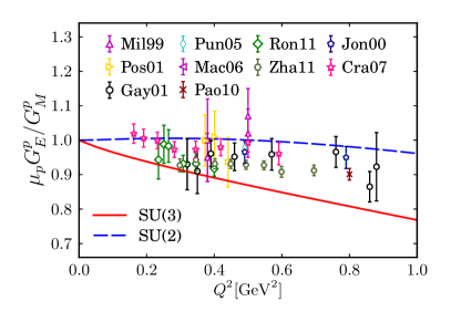
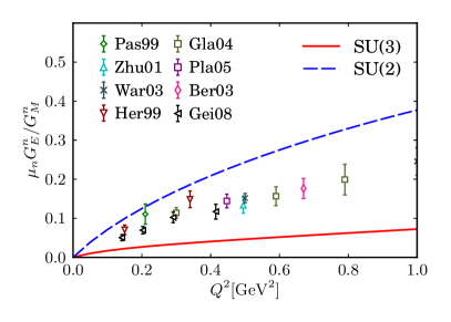
Figure 1: (Color online) The ratio of the proton magnetic FF to the electric FF: $\mu G_{E}/G_{M}$ in the left panel. The experimental data are taken from Mil99 Milbrath:1997de , Pos01 Pospischil:2001pp , Gay01 Gayou:2001qt , Mac06 MacLachlan:2006vw , Pao10 Paolone:2010qc , Ron11 Ron:2011rd , Zha11 Zhan:2011ji , Jon06 Jones:2006kf , Jon00 Jones:1999rz , Cra07 Crawford:2006rz . The neutron $\mu G_{E}/G_{M}$ ratio in the right panel compared to the data from recent experiments: Pas99 Passchier:1999cj , Zhu01 Zhu:2001md , War03 Warren:2003ma , Gei08 Geis:2008aa , Her99 Herberg:1999ud , Gla04 Glazier:2004ny , Pla05 Plaster:2005cx , Ber03 Bermuth:2003qh . The solid curve depicts the result from the SU(3) $\chi$QSM whereas the dashed one does that from the SU(2) model.

In the left panel of Fig. 1, the results of the ratio of the proton magnetic FF to the electric FF are depicted in comparison with the experimental data from the recoil polarisation experiments $p(\vec{e},e^{\prime}\vec{p})$ Jones:1999rz ; Gayou:2001qt ; Puckett:2010ac ; Ron:2011rd ; Zhan:2011ji ; Milbrath:1997de ; Pospischil:2001pp ; MacLachlan:2006vw ; Paolone:2010qc ; Puckett:2011xg and the experiments with a polarised target $\vec{p}(\vec{e},e^{\prime}\vec{p})$ Jones:2006kf ; Crawford:2006rz . The SU(2) results can describe the general tendency of the data very well, whereas those of SU(3) seem slightly underestimated, as $Q^{2}$ increase. The right panel of Fig. 1 plots the results for the ratio $\mu_{n}G_{E}^{n}/G_{M}^{n}$, compared with the experimental data taken from $\vec{d}(\vec{e},en)p$ Passchier:1999cj ; Zhu:2001md ; Warren:2003ma ; Geis:2008aa and from $d(\vec{e},e^{\prime}\vec{n})p$ Herberg:1999ud ; Glazier:2004ny ; Plaster:2005cx and ${}^{3}\vec{\mathrm{He}}(\vec{e},e^{\prime}n)$ scatterings Bermuth:2003qh . We observe that the experimental data lie between the SU(2) and SU(3) results. The general tendency of the present results are in line with the experimental data: $\mu_{p}G_{E}^{p}/G_{M}^{p}$ falls off slowly as $Q^{2}$ increases, while $\mu_{n}G_{E}^{n}/G_{M}^{n}$ increases systematically as a function of $Q^{2}$. As shown in the right panel of Fig 1, the SU(3) results for the neutron are rather different from those in SU(2), the reason stemming, at least partially, from the strange quark contribution to the neutron electric FF. Because of the embedding of the SU(2) soliton into SU(3) as shown in Eq.(15), the contribution of the strange quark has the same asymptotic behavior of the nonstrange quarks. The effects due to different asymptotic tails were discussed in Ref. Silva:2001st in the context of the strange vector FFs of the nucleon. Thus, in a sense, a true answer may be found between the SU(2) and the SU(3) results.

In order to decompose the proton EMFFs into the flavour ones, we need to compute the singlet vector form factors of the proton. Then, we are able to express the flavour-decomposed EMFFs of the proton in terms of the singlet, triplet, and octet FFs of the proton:

$$G_{E,M}^{u}(Q^{2}) = \frac{1}{2}\left(\frac{2}{3}G_{E,M}^{(0)}(Q^{2})+G_{E,M}^{(3)}(Q^{2})+\frac{1}{\sqrt{3}}G_{E,M}^{(8)}(Q^{2})\right),$$ (33)

$$G_{E,M}^{d}(Q^{2}) = \frac{1}{2}\left(\frac{2}{3}G_{E,M}^{(0)}(Q^{2})-G_{E,M}^{(3)}(Q^{2})+\frac{1}{\sqrt{3}}G_{E,M}^{(8)}(Q^{2})\right),$$ (34)

$$G_{E,M}^{s}(Q^{2}) = \frac{1}{3}\left(G_{E,M}^{(0)}(Q^{2})-\sqrt{3}G_{E,M}^{(8)}(Q^{2})\right),$$ (35)

where we have suppressed the corresponding quark charge. The normalisations at $Q^{2}=0$ for the proton obey $G_{E}^{u}(0)=2$, $G_{E}^{d}(0)=1$ and $G_{E}^{s}(0)=0$. The flavour-decomposed magnetic moments are listed in Table 1 in unit of the model nuclear magneton, i.e. defined with the model nucleon mass.

	$\mu_{u}$	$\mu_{d}$	$\mu_{s}$
SU(3)	$3.22$	$-0.73$	$0.10$
SU(2)	$3.46$	$-0.95$
Qattan:2012zf	$3.67$	$-1.03$

Table 1: The flavour-decomposed magnetic moments are defined as $\mu_{q}=G_{M}^{q}(0)$ and are presented in unit of the model nuclear magneton $\mu_{N}$.

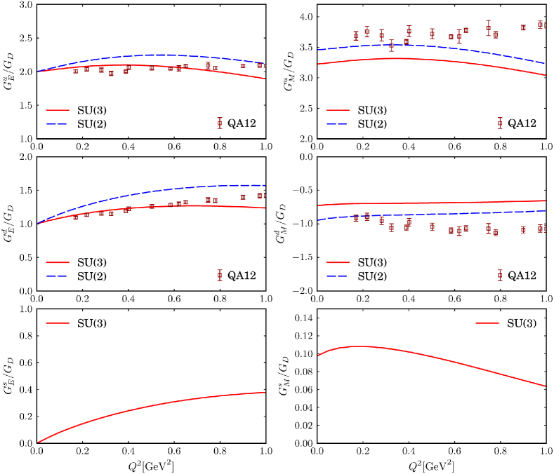
Figure 2: (Color online) Ratios of the nucleon Sachs flavour FFs to the dipole parameterizations (Eq. (36). The $u$ quark FFs in the upper panel, the $d$ quark FFs in the middle panel, and the strange ones in the lower panel. The phenomenological data are taken from Refs. Qattan:2012zf ; Qattan:2012zf:Supplemental (QA12). Notations are the same as in Fig. 1.

The Sachs FFs for the different quark flavours are presented in Fig. 2, which are normalised by the dipole parameterization defined as

$$G_{D}(Q^{2})=\frac{1}{\left(1+\frac{Q^{2}}{\Lambda_{D}^{2}}\right)^{2}},\qquad\Lambda_{D}^{2}=0.71\,\mathrm{GeV}^{2}$$ (36)

in comparison with the phenomenological data taken from Refs. Qattan:2012zf ; Qattan:2012zf:Supplemental , whose normalisations at $Q^{2}=0$ are given as $G_{M}^{u}=3.67\,\mu_{N}$ and $G_{M}^{d}=-1.03\,\mu_{N}$. The up and down electric FFs are more or less well reproduced. On the other hand, the up magnetic FF deviates from the data, as the $Q^{2}$ increases. While the $Q^{2}$ dependence of the down magnetic FF shows similar tendency to the data but the results seem a bit overestimated. Since there are no corresponding experimental data yet for the strange EMFFs, the lower panel of Fig. 2 shows the predictions of the present model for the strange EMFFs.

IV Dirac and Pauli form factors

The Dirac ($F_{1}$) and Pauli ($F_{2}$) FFs are expressed in terms of the Sachs EMFFs inverting Eq. (4), i.e.

$$F_{1}(Q^{2}) = \frac{G_{E}+\tau G_{M}}{1+\tau}$$ (37)

$$F_{2}(Q^{2}) = \frac{G_{M}-G_{E}}{1+\tau},$$ (38)

where $\tau$ is given by

$$\tau=Q^{2}/(4M^{2}).$$ (39)

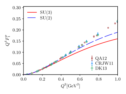
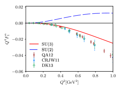
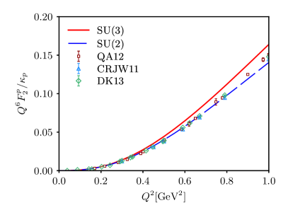
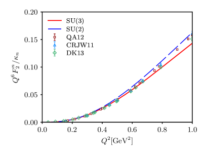
Figure 3: (Color online) Dirac FFs $F_{1}$ of the proton and the neutron, scaled with $Q^{4}$ in the upper panel and the Pauli FFs scaled with $Q^{6}/\kappa_{p(n)}$ in the lower panel. The experimental data are taken from Refs. Cates:2011pz (CRJW11), Qattan:2012zf ; Qattan:2012zf:Supplemental (QA12) and Diehl:2013xca (DK13). Notations are the same as in Fig. 1.

As mentioned in Introduction, pQCD with factorisation schemes Brodsky:1974vy predicts that the nucleon Dirac FFs scale with $1/Q^{4}$. It indicates that $Q^{4}F_{1}(Q^{2})$ becomes asymptotically constant. Thus, the $Q^{4}F_{1}(Q^{2})$ is a more interesting quantity than the $F_{1}$ itself. Figure 3 shows the results for the nucleon Dirac FFs with $Q^{4}$ factor in comparison with the experimental data Cates:2011pz ; Qattan:2012zf ; Diehl:2013xca ; Qattan:2012zf:Supplemental . The $Q^{2}$ dependence of $Q^{4}F_{1}^{p}(Q^{2})$ are well explained within the SU(2) model, while those from the corresponding SU(3) model seem slightly underestimated, especially, as $Q^{2}$ increases. However, as for $Q^{4}F_{1}^{n}(Q^{2})$, the result of the SU(3) model describes the data well, whereas the SU(2) $F_{1}$ turns out positive. As shown in the lower panel of Fig. 3, the results of $Q^{6}F_{2}(Q^{2})/\kappa$ both for the proton and the neutron are in good agreement with the experimental data. However, due to the momentum transfer range, the scaling behaviour is not clear.

The flavour-decomposed Dirac ($F_{1}^{q}$) and Pauli ($F_{2}^{q}$) FFs are expressed as

$$F_{1,2}^{u} = 2F_{1,2}^{p}+F_{1,2}^{n}+F_{1,2}^{s},$$ (40)

$$F_{1,2}^{d} = F_{1,2}^{p}+2F_{1,2}^{n}+F_{1,2}^{s}$$ (41)

in flavour SU(3). In flavour SU(2), the up and down Dirac and Pauli FFs are simply written in terms of the corresponding proton and neutron FFs.

$$F_{1,2}^{u} = 2F_{1,2}^{p}+F_{1,2}^{n},$$ (42)

$$F_{1,2}^{d} = F_{1,2}^{p}+2F_{1,2}^{n}.$$ (43)

Note, however, that $F_{1,2}^{u,d}$ do not turn out the same in SU(3) and SU(2) just by neglecting $F_{1,2}^{s}$ since the flavour groups are different.

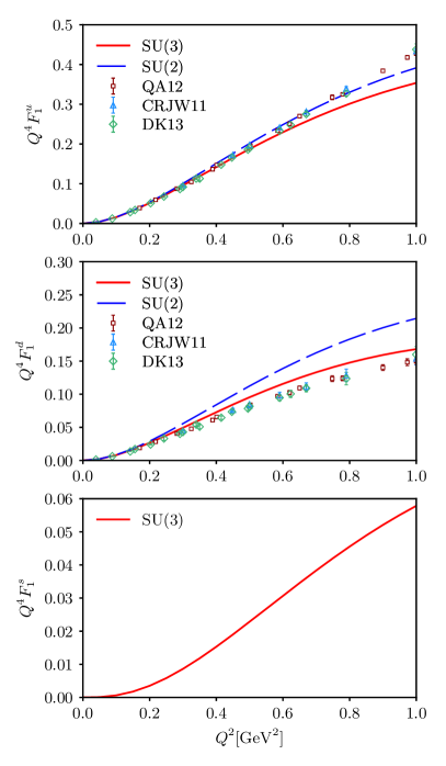
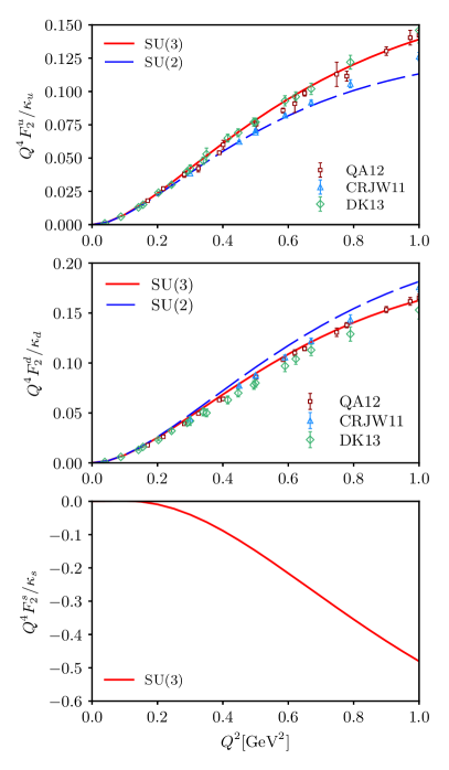
Figure 4: (Color online) The flavour-decomposed Dirac and Pauli FFs weighted by $Q^{4}$: The up FFs in the upper panel, the down ones in the middle panel, and the strange FFs in the lower panel. The experimental data are taken from Refs. Cates:2011pz (CRJW11), Qattan:2012zf ; Qattan:2012zf:Supplemental (QA12) and Diehl:2013xca (DK13). Notations are the same as in Fig. 1.

In Fig. 4, we draw the results of $Q^{4}F_{1}^{q}$ and $Q^{4}F_{2}^{q}/\kappa^{q}$ for the up ($u$), down ($d$) and strange ($s$) quarks, respectively. $Q^{4}F_{1}^{u}$ shows stronger $Q^{2}$ dependence than that of $Q^{4}F_{1}^{d}$ while $Q^{4}F_{2}^{u}$ exhibits weaker $Q^{2}$ dependence than that of $Q^{4}F_{2}^{d}$. The present results for both the up and down quarks describe the data very well as in the case of the proton and neutron FFs (see Fig. 3). Again, we predict $Q^{4}F_{1}^{s}$ and $Q^{4}F_{2}^{s}$.

At $Q^{2}=0$ the Dirac and FFs are respectively reduced to $F_{1}^{p}(0)=1$, $F_{1}^{n}(0)=0$ and $F_{2}^{p(n)}(0)=\kappa_{p(n)}$ with the corresponding anomalous magnetic moment $\kappa_{p(n)}$ (See Table 2). For the flavour-decomposed Dirac FFs, with our normalization $F_{1}^{u}(0)=2$, $F_{1}^{d}(0)=1$ and $F_{1}^{s}(0)=0$.

	$\kappa_{p}$	$\kappa_{n}$	$\kappa_{u}$	$\kappa_{d}$	$\kappa_{s}$
SU(3)	$1.36$	$-1.59$	$1.22$	$-1.73$	$0.10$
SU(2)	$1.62$	$-1.78$	$1.46$	$-1.95$
Exp. & Phen.	$1.793$	$-1.913$	$1.673$	$-2.033$

Table 2: Anomalous magnetic moments $\kappa=F_{2}(0)$ for the proton and the nucleon. The flavour-decomposed anomalous magnetic moments are also presented. Exp. & Phen. denote the experimental data on the proton and the neutron anomalous magnetic moments, and the empirical data on the flavour-decomposed ones.

V Transverse charge densities

We are now in a position to discuss the quark transverse charge densities inside both unpolarised and polarised nucleons. The traditional charge and magnetisation densities in the Breit framework are defined ambiguously because of the Lorentz contraction of the nucleon in its moving direction Kelly:2002if ; Burkardt:2002hr . To avoid this ambiguity one can define the quark charge densities in the transverse plane. Then, they provide essential information on how the charges and magnetisations of the quarks are distributed in the transverse plane. When the nucleon is unpolarised, the quark transverse charge density is defined as the two-dimensional Fourier transform of the nucleon Dirac FFs

$$\rho_{\rm ch}(b)=\frac{1}{(2\pi)^{2}}\int\!d^{2}q\;e^{i{\bm{q}}\cdot{\bm{b}}}F_{1}(Q^{2})=\int_{0}^{\infty}\frac{dQ}{2\pi}\,QJ_{0}(Qb)F_{1}(Q^{2})$$ (44)

where $b$ denotes the impact parameter, i.e. the distance in the transverse plane to the place where the density is being probed, and $J_{0}$ is a cylindrical Bessel Function of order zero Miller:2007uy ; Miller:2010nz . Note that the Dirac FF at $Q^{2}=0$ and the anomalous magnetic moment can be rederived from the transverse charge and magnetisation densities

$$2\pi\!\int\!db\;b\,\rho_{\rm ch}(b)=F_{1}(0),\qquad\pi\!\int\!db\;b\,\rho_{\rm m}(b)=\kappa,$$ (45)

either for the nucleon or for each individual flavour, with the anomalous magnetisation density in the transverse plane defined Miller:2010nz ; Venkat:2010by by

$$\rho_{\rm m}(b)=b\int_{0}^{\infty}\frac{dQ}{2\pi}\,Q^{2}J_{1}(Qb)F_{2}(Q^{2}).$$ (46)

By definition, Eq.s (44,46) seem to imply the knowledge of Dirac and Pauli form factors over a wide range of $Q^{2}$ in order to obtain meaningful densities. This seems at odds with the fact that the present $\chi$CQSM FFs are obtained in the low transferred momenta. However, it turns out that with the model form factors, the integrals in Eq.s (44,46) are saturated in the range $Q^{2}<1.5$ (GeV/c)², i.e. the computed densities do not change when the upper limit in the integrals is set at different values above $1.5$ (GeV/c)².

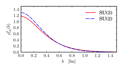
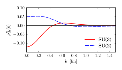
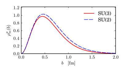
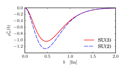
Figure 5: (Color online) Transverse charge densities inside a proton (upper left panel) and a neutron (upper right panel), and the transverse magnetisation densities inside a proton (lower left panel) and a neutron (lower right panel). Notations are the same as in Fig. 1.

In the upper panel of Fig. 5, the transverse charge densities inside both a proton and a neutron are drawn. The results of the transverse charge density from the SU(2) model is almost the same as that from the SU(3) model for the proton. However, it is very interesting to observe that the tranverse charge density inside the neutron from the SU(2) model is opposite to that of the SU(3) one. As already found in Figs. 1 and 3, the SU(2) result is distinguished from the SU(3) one, mainly due to the effects of the strange quark. These are in fact a surprising results, because the SU(3) result interprets the inner structure of the neutron totally differently from the SU(2) one: While the negative charge, which mainly come from the down and strange quarks inside a neutron, is centred on the neutron according to the SU(3) $\chi$QSM, the SU(2) model suggests that the positive one be located in the centre of the neutron. In Ref. Miller:2007uy , the transverse charge density of the neutron was computed, based on the parametrisation of the experimental EMFFs, and was found to be negative in the centre of the neutron, which is in line with the present result from the SU(3) model. To clarify this discrepancy between the SU(2) and the SU(3) models, it might be essential to know the strangeness content of the neutron. We will discuss later each contribution of a quark with different flavour to the transverse charge density inside the neutron more in detail. Another interesting point in the transverse charge density inside a neutron is that it turns positive as $b$ increases. The reason will soon be clear when we discuss the flavour-decomposed transvese charge densities.

The lower panel of Fig. 5 plots the transverse magnetisation densities inside both a proton and a neutron. The results from the SU(2) model are similar to those from the SU(3) model. As expected from their values of the anomalous magnetic moments, the transverse magnetisation densities inside a proton are positive but those inside a neutron turn out to be negative. We will soon observe that the up quark and the down quark contribute oppositely to the magnetisation, which explains the results of the transverse magnetisation densities inside a proton and a neutron.

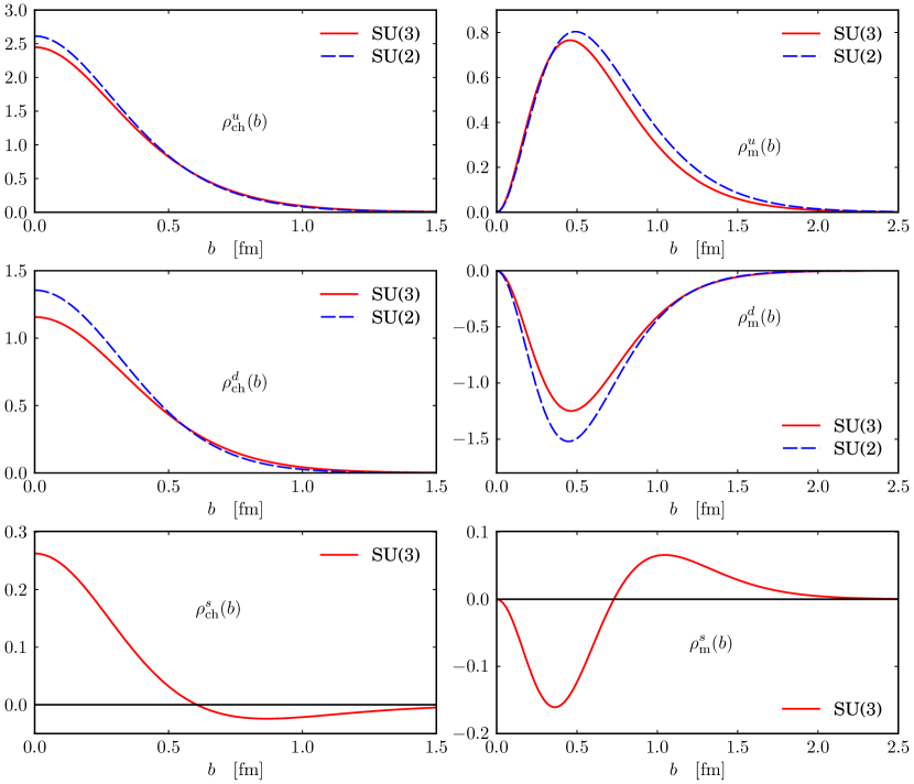
Figure 6: (Color online) Flavour-decomposed transverse charge and magnetisation densities inside a proton. Those for the up quark in the upper panel, the down ones in the middle panel, and the strange charge and magnetisation densities in the lower panel. Notations are the same as in Fig. 1.

In Fig. 6, the transverse charge and magnetisation densities are depicted for each flavour, in the left panel and the right panel, respectively. The results of the transverse densities in Fig. 6 do not include the charges for each flavor. The charge densities for the up and the down quarks look similar to the proton one shown in Fig. 5 and the SU(2) results generally larger in the center region but fall off faster than the SU(3) ones. The strange quark case shows interesting features. While the charge density is found to be positive in the inner region, it becomes negative as $b$ increases. Note that the down quark inside a nucleon is more magnetised than the up quark but was directed opposite to the up quark, which results in the negative larger value of the anomalous magnetic moment for the down quark than for the up quark (see Tab. 2). The strange transverse magnetisation densities look very different from those for the up and down quarks: In the inner part of the nucleon, the strange quark is negatively magnetised. As $b$ increases, the strange magnetisation density turns positive. As a result, the strange anomalous magnetic moment turns out to be small but positive: $\kappa_{s}=0.10$ (see Tab. 2).

As was discussed, the SU(3) transverse charge density was very different from the SU(2) one. We can understand the reason for it from the results of the flavour-decomposed transverse charge densities. The transverse charge densities inside a proton and a neutron can be respectively expressed in terms of the flavour-decomposed ones

$$\rho_{\mathrm{ch}}^{p} = \frac{1}{3}(2\,\rho_{\mathrm{ch}}^{u}-\rho_{\mathrm{ch}}^{d}-\rho_{\mathrm{ch}}^{s}),$$ (47)

$$\rho_{\mathrm{ch}}^{n} = \frac{1}{3}(2\,\rho_{\mathrm{ch}}^{d}-\rho_{\mathrm{ch}}^{u}-\rho_{\mathrm{ch}}^{s}).$$ (48)

Since the $\rho_{\mathrm{ch}}^{u}$ governs the transverse charge density inside a proton ($\rho_{\mathrm{ch}}^{p}$) as shown in Fig. 6, the $\rho_{\mathrm{ch}}^{s}$ has almost negligible effects on it. However, when it comes to the $\rho_{\mathrm{ch}}^{n}$, $2\,\rho_{\mathrm{ch}}^{d}$ and $\rho_{\mathrm{ch}}^{u}$ in Eq. (47) are almost cancelled out each other, which results in a small amount of the negative density. In addition, $\rho_{\mathrm{ch}}^{s}$ contributes negatively to the $\rho_{\mathrm{ch}}^{n}$, which finally leads to the negative value of the $\rho_{\mathrm{ch}}^{n}$ in the centred region, as shown in Fig. 5. In the case of the SU(2) model, the $\rho_{\mathrm{ch}}^{d}$ turns out to be larger than that from the SU(3) model, so that the $\rho_{\mathrm{ch}}^{n}$ becomes positive but tiny. Thus, the strange transverse charge density, though it is small, plays an essential role in explaining the negative value of the $\rho_{\mathrm{ch}}^{n}$ in the centre of the neutron within the framework of the $\chi$QSM. Moreover, the strange transverse charge density turns positive as $b$ increases. This explains partly the reason why the $\rho_{\mathrm{ch}}^{n}$ becomes negative at higher $b$.

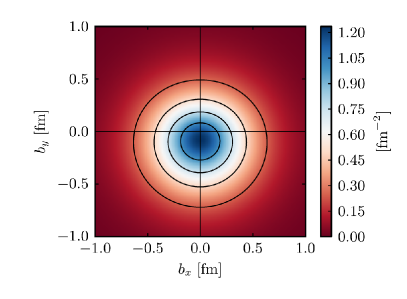
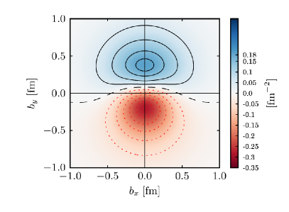
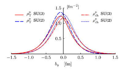
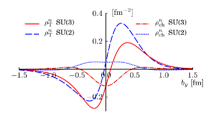
Figure 7: (Color online) Transverse charge densities inside a transversely polarised nucleon. The upper-left and upper-right panels show the transverse charge densities inside a proton and a neutron, respectively, being polarised along the $x$ axis. The lower panel depicts the corresponding transverse charge densities in the $y$ axis with $b_{x}$ fixed ($b_{x}=0$): The solid curve corresponds to the results of the transverse charge densities inside transversely polarised nucleons from the SU(3) model, whereas the dashed curve to those from the SU(2) model. The dotted and dash-dotted curves represent the SU(2) and SU(3) results for the transverse charge densities inside unpolarized nucleons, respectively.

When the nucleon is transversely polarised along the $x$ axis, which can be described by the transverse spin operator of the nucleon $\bm{S}_{\perp}=\cos\phi_{S}\hat{\bm{e}}_{x}+\sin\phi_{S}\hat{\bm{e}}_{y}$, the transverse charge density inside a transversely polarised nucleon is expressed Carlson:2007xd as

$$\rho_{T}(\bm{b})\;=\;\rho_{\mathrm{ch}}(b)-\sin(\phi_{b}-\phi_{S})\frac{1}{2M_{N}b}\rho_{\mathrm{m}}(b),$$ (49)

where $\rho_{\mathrm{m}}(b)$ is given in Eq. (46). The position vector $\bm{b}$ from the centre of the nucleon in the transverse plane is denoted as $\bm{b}=b(\cos\phi_{b}\hat{\bm{e}}_{x}+\sin\phi_{b}\hat{\bm{e}}_{y})$. The $x$ axis is taken as the polarisation direction of the nucleon, i.e. $\phi_{S}=0$. In the upper-left panel of Fig. 7, we plot the transverse charge densities inside a transversely polarised proton. It is shown that the charge density for the transversely polarised proton is distorted in the negative $y$ direction. As discussed in Refs. Burkardt:2002hr ; Carlson:2007xd , the transverse polarisation of the nucleon in the $x$ axis induces the electric dipole moment along the negative $y$ direction, which is a well-known relativistic effect. In the case of the neutron, the situation is even more dramatic. As shown in the upper-right panel of Fig. 5, the negative charge is located at the centre of the neutron with the positive charge surrounding it. However, when the neutron is transversely polarised along the $x$ axis, the negative charge is shifted to the negative $y$ direction but the positive one is moved to the positive $y$ direction. This comes from the fact that the neutron anomalous magnetic moment is negative, which yields an induced electric dipole moment along the positive $y$ axis, as pointed out by Ref. Carlson:2007xd .

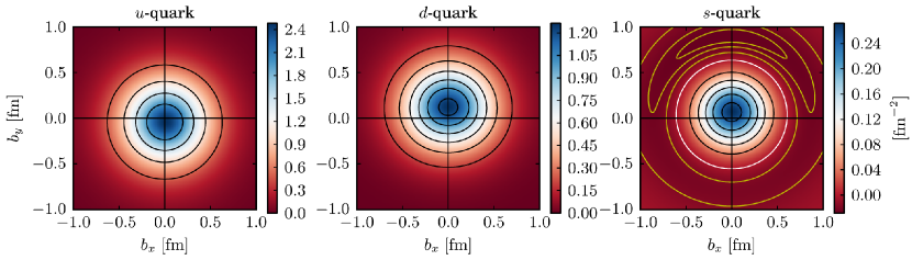
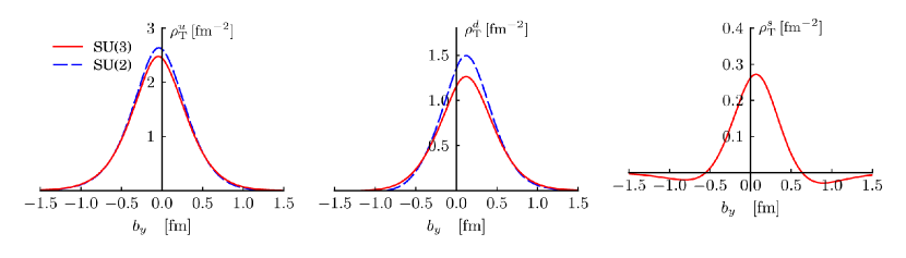
Figure 8: (Color online) Flavor-decomposed transverse charge densities inside a transversely polarised nucleon. The upper-left, the upper-middle and the upper-right panels draw the up, the down, and the strange transverse charge densities inside a proton and a neutron, respectively, being polarised along the $x$ axis. The lower panel depicts the corresponding transverse charge densities in the $y$ axis with $b_{x}$ fixed ($b_{x}=0$). Notations are the same as in Fig. 1.

It is very instructive to examine the transverse charge densities inside the transversely polarised nucleon for each flavour, since they reveal with more detail the inner structure of the nucleon. Figure 8 illustrates them. The up transverse charge density inside the transversely polarised nucleon, $\rho_{T}^{u}$ is shown to be shifted to the negative direction, while that for the down quark is more distorted upwards. It is natural, since the up and down quarks have positive and negative charges, respectively. However, it is remarkable to see that the down quark is influenced more strongly due to the transverse polarisation of the nucleon. The $\rho_{T}^{s}$ is even more interesting. As discussed previously, the strange anomalous magnetic moment is $\kappa_{s}=+0.10$, which would induce the negative electric dipole moment along the negative $b_{y}$. However, situation turns out to be more complicated. As shown in the right panel of Fig. 8, the $\rho_{T}^{s}$ is shifted to the positive $b_{y}$ and turns negative starting from $b_{y}\approx 0.7\,\mathrm{fm}$. In order to understand this surprising result, we need to reexamine the transverse magnetisation density for the strange quark, which has been presented in Fig. 6. The strange magnetisation density is negative in the inner part of the nucleon and then it becomes positive from $b\approx 0.7\,\mathrm{fm}$. Thus, the electric dipole moment is correspondingly induced along the positive $y$ direction in the centred region, and then it becomes negative from $b\approx 0.7\,\mathrm{fm}$, as drawn in the right panel of Fig. 8.

VI Summary and conclusion

In the present work, we aimed at investigating the electromagnetic properties of the nucleon, based on the SU(2) and SU(3) chiral quark-soliton model with a symmetry-preserving quantisation employed. We considered the rotational $1/N_{c}$ corrections and the first-order $m_{s}$ corrections. It should be stressed at this point that no free parameters were used in this work. The only model parameter to be constrained in the baryon sector, namely the constituent quark mass, was taken from previous studies with various observables.

We first presented the results of the ratio of the magnetic form factor to the electric form factor of the proton. It was shown that the results from the SU(2) chiral quark-soliton model described the experimental data very well, whereas those of SU(3) seemed slightly underestimated in higher $Q^{2}$. The general tendency of the present results were in greement with the experimental data. As for the neutron, the SU(3) results turned out to be rather different from those in SU(2), which arose from the strange quark contribution to the neutron electric form factor. In particular, the neutron electric form factor is rather sensitive to the tail of the soliton. We then discussed that the up and the down electric form factors normalised by the dipole parametrisation were well reproduced in comparison with the data. As for the magnetic form factors, they deviate from the experimental data as $Q^{2}$ increases but the general behaviour of the form factors are in line with the experimental data, which indicates that the $Q^{2}$ dependence are well explained. We presented the prediction of the strange form factors normalised by the dipole form factor.

The Dirac and Pauli form factors were predicted to be asymptotically proportional to $1/Q^{4}$ and $1/Q^{6}$ respectively in perturbative QCD. Thus, we studied $Q^{4}F_{1}(Q^{2})$ and $Q^{6}F_{2}(Q^{2})$ in order to compare their $Q^{2}$ dependence with the experimental data. We found that the present SU(2) model explained well $Q^{4}F_{1}^{p}(Q^{2})$ whereas the result from the SU(3) model becomes underestimated at higher $Q^{2}$. Both the SU(2) and SU(3) results for $Q^{6}F_{2}^{p,n}(Q^{2})/\kappa_{p,n}$ described the experimental data very well. On the other hand, the SU(2) result for $Q^{4}F_{1}^{n}$ is in conflict with the data, but that from the SU(3) model is in agreement with the data except for the higher $Q^{2}$ region. Again this discrepancy can be understood by the sensitivity of the neutron electric form factor to the soliton tail. The results for the flavour-decomposed $Q^{4}F_{1}(Q^{2})$ and $Q^{6}F_{2}(Q^{2})$ were shown to be generally in good agreement with the corresponding values from the experimental data.

Having performed the two-dimensional Fourier transform of the nucleon electromagnetic form factors, we were able to produce the charge densities in the transverse plane inside a proton. As expected, both the SU(2) and the SU(3) transverse charge densities were positive in the proton. However, as for the neutron case, the result from the SU(2) was opposite to that from the SU(3): the negative charge was located in the centre of the neutron while the positive one was distributed in outer part within the SU(3) chiral quark-soliton model, it was other way around in the SU(2) model. The explanation comes from the decomposed-flavour transverse charge densities in the SU(3) model. In particular, the component of the strange quark played an essential role in spite of the smallness of its magnitude. Since the up quark component mainly contributed to the transverse charge density inside a proton, the strange transverse charge density was almost negligible. On the other hand, the up and the down quark contributions were nearly cancelled out in such a way that the negative charge remained in the centre of the neutron with small magnitude. Then the contribution of the strange quark came into play, so that the transverse charge densities inside a neutron finally became negative in the centre.

When the proton was polarised along the positive $x$ direction, the corresponding transverse charge density was shifted to the negative $y$ direction, which indicated that the electric dipole moment was induced along the negative $y$ direction. It is just a well-known relativistic effect in electrodynamics. In the case of the neutron polarised along the $x$ axis, the negative charge was moved to the negative $y$ direction but the positive one was forced to the positive $y$ axis. It implies that the neutron anomalous magnetic moment is negative, which induces an electric dipole moment along the positive $y$ axis. We also decomposed the transverse charge densities inside the polarised nucleon for each flavour: the up transverse charge density for the nucleon transversely polarised along the positive $x$ axis was found to be shifted to the negative direction, while that of the down quark was more distorted upwards. Since the up and down quarks have positive and negative charges, respectively, one can easily understand these features. However, the down quark was found to be affected more strongly due to the transverse polarisation of the nucleon. The strange charge density inside the transversely polarised nucleon was shifted to the positive $b_{y}$ and turned out to be negative in the outer region. This unexpected behavior of the strange charge density for the transversely polarised nucleon was explained in terms of the strange magnetisation density.

Since the transverse charge densities inside unpolarised and polarised nucleons pave the novel way for understanding the internal structure of the nucleon, it is interesting to investigate them for other baryons such as the $\Delta$ isobar and hyperons. The transverse charge densities are directly connected to the generalized parton distributions of which the integrations over parton momentum fractions yield form factors and consequently the spatial distribution of partons in the transverse plane. Moreover, the transverse charge densities for transition form factors provide a new aspect of understanding the inner structure of the baryons. For example, as Ref. Carlson:2007xd already studied, they exhibit explicitly multipole structures of the transitions in the transverse plane. Thus, it is of great importance to examine the transverse charge densities for other baryons and for their transitions. Corresponding investigations are under way.

References

- (1) M. K. Jones et al. [Jefferson Lab Hall A Collaboration], Phys. Rev. Lett. 84, 1398 (2000) [nucl-ex/9910005].
- (2) O. Gayou et al. [Jefferson Lab Hall A Collaboration], Phys. Rev. C 64, 038202 (2001).
- (3) O. Gayou et al. [Jefferson Lab Hall A Collaboration], Phys. Rev. Lett. 88, 092301 (2002) [nucl-ex/0111010].
- (4) V. Punjabi et al. [Jefferson Lab Hall A Collaboration], Phys. Rev. C 71, 055202 (2005) [Erratum-ibid. C 71, 069902 (2005)] [nucl-ex/0501018].
- (5) A. J. R. Puckett, E. J. Brash, M. K. Jones, W. Luo, M. Meziane, L. Pentchev, C. F. Perdrisat and V. Punjabi et al., Phys. Rev. Lett. 104, 242301 (2010) [arXiv:1005.3419 [nucl-ex]].
- (6) J. C. Bernauer et al. [A1 Collaboration], Phys. Rev. Lett. 105, 242001 (2010) [arXiv:1007.5076 [nucl-ex]].
- (7) G. Ron et al. [Jefferson Lab Hall A Collaboration], Phys. Rev. C 84, 055204 (2011) [arXiv:1103.5784 [nucl-ex]].
- (8) X. Zhan, K. Allada, D. S. Armstrong, J. Arrington, W. Bertozzi, W. Boeglin, J. -P. Chen and K. Chirapatpimol et al., Phys. Lett. B 705, 59 (2011) [arXiv:1102.0318 [nucl-ex]].
- (9) C. E. Hyde-Wright and K. de Jager, Ann. Rev. Nucl. Part. Sci. 54, 217 (2004) [nucl-ex/0507001].
- (10) J. Arrington, C. D. Roberts and J. M. Zanotti, J. Phys. G 34, S23 (2007) [nucl-th/0611050].
- (11) C. F. Perdrisat, V. Punjabi and M. Vanderhaeghen, Prog. Part. Nucl. Phys. 59, 694 (2007) [hep-ph/0612014].
- (12) M. Vanderhaeghen and T. Walcher, arXiv:1008.4225 [hep-ph].
- (13) J. Arrington, K. de Jager and C. F. Perdrisat, J. Phys. Conf. Ser. 299, 012002 (2011) [arXiv:1102.2463 [nucl-ex]].
- (14) P. A. M. Guichon and M. Vanderhaeghen, Phys. Rev. Lett. 91, 142303 (2003) [hep-ph/0306007].
- (15) P. G. Blunden, W. Melnitchouk and J. A. Tjon, Phys. Rev. Lett. 91, 142304 (2003) [nucl-th/0306076].
- (16) J. Arrington, Phys. Rev. C 71, 015202 (2005) [hep-ph/0408261].
- (17) J. Arrington, W. Melnitchouk and J. A. Tjon, Phys. Rev. C 76, 035205 (2007) [arXiv:0707.1861 [nucl-ex]].
- (18) C. E. Carlson and M. Vanderhaeghen, Ann. Rev. Nucl. Part. Sci. 57, 171 (2007) [hep-ph/0701272 [HEP-PH]].
- (19) J. Arrington, P. G. Blunden and W. Melnitchouk, Prog. Part. Nucl. Phys. 66, 782 (2011) [arXiv:1105.0951 [nucl-th]].
- (20) S. J. Brodsky and G. R. Farrar, Phys. Rev. D 11, 1309 (1975).
- (21) B. Aubert et al. [BABAR Collaboration], Phys. Rev. D 80, 052002 (2009) [arXiv:0905.4778 [hep-ex]].
- (22) S. Uehara et al. [Belle Collaboration], Phys. Rev. D 86, 092007 (2012) [arXiv:1205.3249 [hep-ex]].
- (23) G. D. Cates, C. W. de Jager, S. Riordan and B. Wojtsekhowski, Phys. Rev. Lett. 106, 252003 (2011) [arXiv:1103.1808 [nucl-ex]].
- (24) I. A. Qattan and J. Arrington, Phys. Rev. C 86, 065210 (2012) [arXiv:1209.0683 [nucl-ex]].
- (25) I. A. Qattan, J. Arrington and A. Alsaad, Phys. Rev. C 91, no. 6, 065203 (2015) [arXiv:1502.02872 [nucl-ex]].
- (26) M. Diehl and P. Kroll, Eur. Phys. J. C 73, no. 4, 2397 (2013) [arXiv:1302.4604 [hep-ph]].
- (27) I. C. Cloet, G. Eichmann, B. El-Bennich, T. Klahn and C. D. Roberts, Few Body Syst. 46, 1 (2009) [arXiv:0812.0416 [nucl-th]].
- (28) C. Crawford et al., Phys. Rev. C 82, 045211 (2010) [arXiv:1003.0903 [nucl-th]].
- (29) S. Riordan et al., Phys. Rev. Lett. 105, 262302 (2010) [arXiv:1008.1738 [nucl-ex]].
- (30) G. Eichmann, Phys. Rev. D 84, 014014 (2011) [arXiv:1104.4505 [hep-ph]].
- (31) M. Rohrmoser, K. -S. Choi and W. Plessas, arXiv:1110.3665 [hep-ph].
- (32) M. Rohrmoser, K. S. Choi and W. Plessas, Few Body Syst. 58, no. 2, 83 (2017) doi:10.1007/s00601-017-1243-0 [arXiv:1701.07337 [hep-ph]].
- (33) I. C. Cloet and G. A. Miller, Phys. Rev. C 86, 015208 (2012) [arXiv:1204.4422 [nucl-th]].
- (34) J. O. Gonzalez-Hernandez, S. Liuti, G. R. Goldstein and K. Kathuria, Phys. Rev. C 88, no. 6, 065206 (2013) [arXiv:1206.1876 [hep-ph]].
- (35) D. Chakrabarti and C. Mondal, Eur. Phys. J. C 73, 2671 (2013) [arXiv:1307.7995 [hep-ph]].
- (36) C. Mondal and D. Chakrabarti, Eur. Phys. J. C 75, no. 6, 261 (2015) [arXiv:1501.05489 [hep-ph]].
- (37) C. Mondal, Phys. Rev. D 94, no. 7, 073001 (2016) [arXiv:1609.07759 [hep-ph]].
- (38) N. Sharma, Eur. Phys. J. A 52, no. 11, 338 (2016) [arXiv:1610.07745 [hep-ph]].
- (39) N. S. Nikkhoo and M. R. Shojaei, Int. J. Mod. Phys. E 24, no. 11, 1550086 (2015).
- (40) S. J. Brodsky, R. F. Lebed and V. E. Lyubovitskij, Phys. Lett. B 764, 174 (2017) [arXiv:1609.06635 [hep-ph]].
- (41) I. T. Obukhovsky, A. Faessler, T. Gutsche and V. E. Lyubovitskij, J. Phys. G 41, 095005 (2014).
- (42) D. Chakrabarti and C. Mondal, Eur. Phys. J. C 74, 2962 (2014) [arXiv:1402.4972 [hep-ph]].
- (43) N. Sharma, Phys. Rev. D 90, no. 9, 095024 (2014) [arXiv:1411.7486 [hep-ph]].
- (44) D. Diakonov, V. Y. Petrov and P. V. Pobylitsa, Nucl. Phys. B 306, 809 (1988).
- (45) M. Wakamatsu and H. Yoshiki, Nucl. Phys. A 524, 561 (1991).
- (46) A. Blotz, D. Diakonov, K. Goeke, N. W. Park, V. Y. Petrov and P. V. Pobylitsa, Nucl. Phys. A 555, 765 (1993).
- (47) R. Alkofer, H. Reinhardt and H. Weigel, Phys. Rept. 265, 139 (1996).
- (48) C. V. Christov, A. Blotz, H. -Ch. Kim, P. Pobylitsa, T. Watabe, T. Meissner, E. Ruiz Arriola and K. Goeke, Prog. Part. Nucl. Phys. 37, 91 (1996) [hep-ph/9604441].
- (49) H. Weigel, Lect. Notes Phys. 743, 1 (2008).
- (50) K. Goeke, M. V. Polyakov and M. Vanderhaeghen, Prog. Part. Nucl. Phys. 47, 401 (2001) [hep-ph/0106012].
- (51) K. Goeke, H. -Ch. Kim, A. Silva and D. Urbano, Eur. Phys. J. A 32, 393 (2007) [hep-ph/0608262].
- (52) A. Silva, H. -Ch. Kim, D. Urbano and K. Goeke, Phys. Rev. D 74, 054011 (2006) [hep-ph/0601239].
- (53) H. -Ch. Kim, A. Blotz, M. V. Polyakov and K. Goeke, Phys. Rev. D 53, 4013 (1996) [hep-ph/9504363].
- (54) M. Praszałowicz, T. Watabe and K. Goeke, Nucl. Phys. A 647, 49 (1999) [hep-ph/9806431].
- (55) E. Witten, Nucl. Phys. B 160, 57 (1979) and
- (56) E. Witten, Nucl. Phys. B 223, 422 (1983) and Nucl. Phys. B 223, 433 (1983).
- (57) G. S. Yang, H.-Ch. Kim, M. V. Polyakov and M. Praszałwicz, Phys. Rev. D 94, 071502 (2016) doi:10.1103/PhysRevD.94.071502 [arXiv:1607.07089 [hep-ph]].
- (58) H.-Ch. Kim, M. V. Polyakov and M. Praszałowicz, Phys. Rev. D 96, no. 1, 014009 (2017) Addendum: [Phys. Rev. D 96, no. 3, 039902 (2017)] doi:10.1103/PhysRevD.96.039902, 10.1103/PhysRevD.96.014009 [arXiv:1704.04082 [hep-ph]].
- (59) H.-Ch. Kim, M. V. Polyakov, M. Praszalowicz and G. S. Yang, Phys. Rev. D 96, no. 9, 094021 (2017) doi:10.1103/PhysRevD.96.094021 [arXiv:1709.04927 [hep-ph]].
- (60) D. Androic et al. [G0 Collaboration], Phys. Rev. Lett. 104, 012001 (2010) [arXiv:0909.5107 [nucl-ex]].
- (61) X. -D. Ji, J. Phys. G 24, 1181 (1998) [hep-ph/9807358].
- (62) M. Diehl, Phys. Rept. 388, 41 (2003) [hep-ph/0307382].
- (63) A. V. Belitsky and A. V. Radyushkin, Phys. Rept. 418, 1 (2005) [hep-ph/0504030].
- (64) F. J. Ernst, R. G. Sachs, and K. C. Wali, Phys. Rev. 119, 1105 (1960).
- (65) R. G. Sachs, Phys. Rev. 126, 2256 (1962).
- (66) R. G. Arnold, C. E. Carlson, and F. Gross, Phys. Rev. C 23, 363 (1981).
- (67) G. A. Miller, Phys. Rev. Lett. 99, 112001 (2007) [arXiv:0705.2409 [nucl-th]].
- (68) G. A. Miller, Ann. Rev. Nucl. Part. Sci. 60, 1 (2010) [arXiv:1002.0355 [nucl-th]].
- (69) S. Venkat, J. Arrington, G. A. Miller and X. Zhan, Phys. Rev. C 83, 015203 (2011) [arXiv:1010.3629 [nucl-th]].
- (70) B. D. Milbrath et al. [Bates FPP Collaboration], Phys. Rev. Lett. 80 (1998) 452 [Erratum-ibid. 82 (1999) 2221] [nucl-ex/9712006].
- (71) T. Pospischil et al. [A1 Collaboration], Eur. Phys. J. A 12, 125 (2001).
- (72) G. MacLachlan, A. Aghalarian, A. Ahmidouch, B. D. Anderson, R. Asaturian, O. Baker, A. R. Baldwin and D. Barkhuff et al., Nucl. Phys. A 764, 261 (2006).
- (73) M. Paolone, S. P. Malace, S. Strauch, I. Albayrak, J. Arrington, B. L. Berman, E. J. Brash and W. J. Briscoe et al., Phys. Rev. Lett. 105, 072001 (2010) [arXiv:1002.2188 [nucl-ex]].
- (74) A. J. R. Puckett, E. J. Brash, O. Gayou, M. K. Jones, L. Pentchev, C. F. Perdrisat, V. Punjabi and K. A. Aniol et al., Phys. Rev. C 85, 045203 (2012) [arXiv:1102.5737 [nucl-ex]].
- (75) M. K. Jones et al. [Resonance Spin Structure Collaboration], Phys. Rev. C 74, 035201 (2006) [nucl-ex/0606015].
- (76) C. B. Crawford, A. Sindile, T. Akdogan, R. Alarcon, W. Bertozzi, E. Booth, T. Botto and J. Calarco et al., Phys. Rev. Lett. 98, 052301 (2007) [nucl-ex/0609007].
- (77) I. Passchier, R. Alarcon, T. S. Bauer, D. Boersma, J. F. J. van den Brand, L. D. van Buuren, H. J. Bulten and M. Ferro-Luzzi et al., Phys. Rev. Lett. 82, 4988 (1999) [nucl-ex/9907012].
- (78) H. Zhu et al. [Jefferson Lab E93-026 Collaboration], Phys. Rev. Lett. 87, 081801 (2001) [nucl-ex/0105001].
- (79) G. Warren et al. [Jefferson Lab E93-026 Collaboration], Phys. Rev. Lett. 92, 042301 (2004) [nucl-ex/0308021].
- (80) E. Geis et al. [BLAST Collaboration], Phys. Rev. Lett. 101, 042501 (2008) [arXiv:0803.3827 [nucl-ex]].
- (81) C. Herberg, M. Ostrick, H. G. Andresen, J. R. M. Annand, K. Aulenbacher, J. Becker, P. Drescher and D. Eyl et al., Eur. Phys. J. A 5, 131 (1999).
- (82) D. I. Glazier et al. [A1 Collaboration], Eur. Phys. J. A 24, 101 (2005) [nucl-ex/0410026].
- (83) B. Plaster et al. [Jefferson Lab E93-038 Collaboration], Phys. Rev. C 73, 025205 (2006) [nucl-ex/0511025].
- (84) J. Bermuth, P. Merle, C. Carasco, D. Baumann, D. Bohm, D. Bosnar, M. Ding and M. O. Distler et al., Phys. Lett. B 564, 199 (2003) [nucl-ex/0303015].
- (85) A. Silva, H. -Ch. Kim and K. Goeke, Phys. Rev. D 65, 014016 (2002) [Erratum-ibid. D 66, 039902 (2002)] [hep-ph/0107185].
- (86) Supplemental Material from Qattan:2012zf at http://link.aps.org/supplemental/10.1103/PhysRevC.86.065210
- (87) J. J. Kelly, Phys. Rev. C 66, 065203 (2002) [hep-ph/0204239].
- (88) M. Burkardt, Int. J. Mod. Phys. A18 (2003) 173-208. [arXiv:hep-ph/0207047 [hep-ph]].
- (89) C. E. Carlson and M. Vanderhaeghen, Phys. Rev. Lett. 100, 032004 (2008) [arXiv:0710.0835 [hep-ph]].