Multiple testing of local maxima for detection of peaks in ChIP-Seq data

Abstract

A topological multiple testing approach to peak detection is proposed for the problem of detecting transcription factor binding sites in ChIP-Seq data. After kernel smoothing of the tag counts over the genome, the presence of a peak is tested at each observed local maximum, followed by multiple testing correction at the desired false discovery rate level. Valid $p$-values for candidate peaks are computed via Monte Carlo simulations of smoothed Poisson sequences, whose background Poisson rates are obtained via linear regression from a Control sample at two different scales. The proposed method identifies nearby binding sites that other methods do not.

, , and t1Supported in part by the Claudia Adams Barr Program in Cancer Research, the William F. Milton Fund and NIH Grants P01-CA134294 and R01-CA157528. t2Supported in part by T32 GM074906 Predoctoral Biostatistics Training in Genetics/Genomics.

1 Introduction

The problem of detecting signal peaks in the presence of background noise appears often in the analysis of high-throughput data. In ChIP-Seq data, the problem of finding transcription factor binding sites along the genome translates to a large-scale peak detection problem with a one-dimensional spatial structure, where the number, locations and heights of the peaks are unknown. Recently, Schwartzman, Gavrilov and Adler (2011) (hereafter SGA) introduced a topological multiple testing approach to peak detection where, after kernel smoothing, the presence of a signal is tested not at each spatial location but only at the local maxima of the smoothed observed sequence. In this paper, we show how that approach can be used to formalize the inference problem of finding binding sites in ChIP-Seq data. To achieve this, we also propose a new regression-based method for estimating the local background binding rate from a Control sample.

1.1 ChIP-Seq data

ChIP-Sequencing or ChIP-Seq is an experimental method that is often used to map the locations of binding sites of transcription factors along the genome in vivo [Barski and Zhao (2009), Park (2009)]. Transcription factors control the transcription of genetic information from DNA to mRNA in living cells, and abnormalities in this process are often associated with cancer. Given a particular transcription factor of interest, ChIP-Seq combines chromatin immunoprecipitation (ChIP) with massively parallel DNA sequencing, allowing enrichment of the DNA segments bound by the transcription factor and mapping of their locations along the genome. The result is a long list of sequenced forward and reverse tags, also called reads, each associated with a specific genomic address. After alignment of these tags, the data consists of a sequence of tag counts along the genome, with a tendency to a higher concentration of tags near the transcription factor binding sites. An example of a data fragment is shown in Rows 1 and 2 of Figure 1. (Note that not all ChIP-Seq data follow this pattern, e.g., histone modification data.)

The goal of the analysis is to identify the true binding sites. This translates to finding genomic locations where the binding rate is higher than it would be if the transcription factor were not present. To this end, Johnson et al. (2007) suggested sequencing a Control input sample to provide an experimental assessment of the background tag distribution, helping reduce false positives. The cost currently associated with this technology often does not allow more than a single ChIP-Seq sample, also called an IP sample, and a single Control sample. To illustrate the usefulness of the Control, Rows 1 and 2 of Figure 1 show a short fragment of the raw data after alignment in the Control and IP samples, respectively, for the same positions in the genome. The interesting peaks are marked by red circles in Row 3, corresponding to sites with high binding rate in the IP sample but lower rate in the Control. Other candidate peaks, marked in blue, do not have a significantly higher binding rate in the IP sample than in the Control.

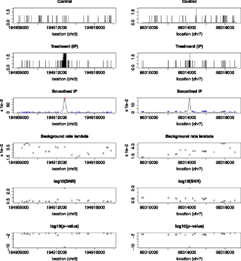
Figure 1: A fragment of the Fox A1 aligned data featuring a few representative peaks found by our method. Row 1: Control sample. Row 2: IP sample, same fragment as the Control. Row 3: Smoothed IP sample; significant peaks are indicated in red, nonsignificant ones in blue. Row 4: Estimates of the background Poisson rate $\lambda_{0}(t)$ at local maxima of the smoothed IP sample. Row 5: Signal-to-noise ratio (SNR), equal to peak height divided by background rate (log 10 scale). Row 6: $P$-values (log 10 scale). Notice the difference in vertical scales between the left and right panels.

As an additional condition, it is necessary that a site has a high binding rate in absolute terms to avoid spurious high fold enrichments due to high variability at low coverage (e.g., 3-fold enrichment resulting from 3 reads in treatment vs. 1 read in control).

1.2 Testing of local maxima

The search for binding sites may be set up as a large-scale multiple testing problem where, at each genomic location, a test is performed for whether the binding rate is higher than the background. Testing at each genomic location is statistically inefficient because it requires a multiple testing correction for a very large number of tests over the entire length of the genome. In ChIP-Seq, the binding rate at a true binding site has a unimodal peak shape that spreads into neighboring locations, caused by the variability in the start and end points of the sequenced segments. Thus, as argued by SGA, it is enough to test for high binding rates only at locations that resemble peaks, that is, local maxima of the smoothed data. In this sense, the local maxima serve as topological representatives of the candidate binding sites.

Peak detection on the aligned data is carried out using the Smooth and Test Local Maxima (STEM) algorithm of SGA. It consists of the following: [(1)]

kernel smoothing;

finding the local maxima as candidate peaks;

computing $p$-values for the heights of the observed local maxima; and

applying a multiple testing procedure to the obtained $p$-values. For Step 1, following the “matched filter principle” recommended by SGA, we use a symmetric unimodal kernel that roughly matches the shape of the peaks to be detected. This shape corresponds to the spatial spread of tag locations around a true binding site and is assumed to be the same for all binding sites, up to an amplitude scaling factor dictated by the physics and chemistry of the experimental protocol. This shape, up to an amplitude scaling factor, is estimated from the data during the alignment process. In Step 2, local maxima are defined as smoothed counts that are higher than their neighbors after correcting for ties. In Step 3, $p$-values test the hypothesis that the local binding rate is less or equal to the local background rate or a minimally interesting binding rate. The required distribution of the heights of local maxima is computed via Monte Carlo simulations. Finally, Step 4 is carried out using the Benjamini–Hochberg (BH) procedure [Benjamini and Hochberg (1995)], although, in general, other multiple testing algorithms may be used instead.

The STEM algorithm is promising for ChIP-Seq data because it was shown in SGA to provide asymptotic error control and power consistency under similar modeling assumptions. Like in ChIP-Seq data, SGA assumed that the signal peaks are unimodal with finite support and that the search occurs over a long observed sequence. Further assuming additive Gaussian stationary ergodic noise, SGA proved that the BH procedure controls the false discovery rate (FDR) of detected peaks, defined as the expected ratio of falsely detected peaks among detected peaks, where a detected peak is considered true (false) if it occurs inside (outside) the support of any true peak. In SGA, the control is asymptotic as both the search space and the signal strength increase, where the former may grow exponentially faster than the latter, and the detection power tends to one under the same asymptotic conditions. In ChIP-Seq data, the definitions of true and false detected peaks apply within the spatial extent of the true peak shape, which is estimated here during the alignment process.

1.3 Estimation of the background rate and Monte Carlo calculation of $p$-values

ChIP-Seq data differs from the modeling assumptions of SGA in that ChIP-Seq data consists of a long sequence of positive integer counts, often assumed to follow a Poisson distribution [Mikkelsen et al. (2007)]. Moreover, the process generating the background noise counts is not globally stationary [Johnson et al. (2007)]. To make inference possible, we assume the background Poisson rate to vary over the genome but not too fast so that it is approximately constant in the immediate vicinity of any candidate peak. The background Poisson rate at any given location is estimated as a linear function of the local Control counts at two different spatial scales, 1 kilo base-pairs (kb) and 10 kb. The linear coefficients are estimated from the data by multiple regression, automatically solving the normalization problem of having different sequencing depths between the IP and Control samples.

Finally, as required by Step 3 of the STEM algorithm above, for an observed local maximum of the smoothed ChIP-Seq data at a given location, its $p$-value is computed via Monte Carlo simulation using the background Poisson parameter estimated for that location. Note that the STEM algorithm requires an estimate of the background, but does not depend on how that estimate was obtained. Here we propose a regression method, but that method could be changed without changing the basic operation of the STEM algorithm.

1.4 Other methods

Several ChIP-Seq data analysis methods have been proposed in the literature; cf. MACS [Zhang et al. (2008)], cisGenome [Ji et al. (2008)], QuEST [Valouev et al. (2008)] and FindPeaks [Fejes et al. (2008)]. While these methods also view the problem of detecting binding sites as a peak detection problem, use statistical models and estimate error rates, most of them do not formally state the statistical inference problem. Exceptions are PICS [Zhang et al. (2011)] and BayesPeak [Spyrou et al. (2009)], which are both Bayesian approaches, whereas we adopt a frequentist point of view. QuEST [Valouev et al. (2008)] also finds local maxima as candidate peaks but uses a narrow Gaussian kernel rather than a matched filter and estimates the FDR by comparing the number of peaks called in the IP and Control sequences rather than estimating the background and formally testing using $p$-values. T-PIC [Hower, Evans and Pachter (2011)] also takes a topological approach, but rather than heights of local maxima it measures the depth of trees built from excursion regions of the coverage function of the data, so our method is simpler.

Here we attempt to frame the ChIP-Seq analysis problem as a formal inference problem in multiple testing relying on the error control properties proven in SGA and using a new regression method to estimate the background binding rate. As a reference, we compare the results of our analysis to those of MACS, cisGenome and QuEST on two different data sets. By focusing on detecting peaks rather than regions and using a matched filter, our approach has the ability to distinguish nearby binding sites that MACS and ciSGenome do not, and in a less fragmented fashion than QuEST.

1.5 Data sets

We demonstrate our approach on two different ChIP-Seq data sets. In the first, ChIP-Seq targeting the transcription factor FoxA1 was performed on the breast cancer cell line MCF-7 [Zhang et al. (2008)]. This data set includes a ChIP-Seq sample (hereafter IP), in which the FoxA1 antibody was used, and a Control input sample, in which the procedure was repeated without the antibody. Sequencing covered the entire genome, producing about 3.9 million tags in the IP sample and about 5.2 million tags in the Control sample. The second data set concerns the growth-associated binding protein (GABP) [Valouev et al. (2008)]. This larger data set consists of an IP sample with about 7.8 million tags and a Control sample with about 17.4 million tags. The methods in this paper were developed on the FoxA1 data set and later applied to the GABP data set as an independent testbed. In both data sets, the goal of the analysis is to detect genomic loci in the IP sample that have a significantly high number of tags both in absolute terms and relative to the Control sample.

It should be noted that the goal of this paper is not to propose a new peak finding tool, but rather to show how a topological inference approach can be used to provide formal statistical inference in ChIP-Seq data, with the view that its basic principles can be generalized to other genomic search problems [Jaffe et al. (2012)]. The methods in this paper were implemented in R.

2 Peak detection for ChIP-Seq data

2.1 Alignment and estimation of the peak shape

Before statistical analysis, we follow the approach in MACS of first aligning the forward and reverse tags, after which tags can be treated indistinctively. The alignment process, described in the Appendix, also allows us to estimate the amount by which tags need to be shifted and the shape of the spatial spread of the shifted tag counts around a peak.

For illustration, Figure 2(a) shows the spatial distributions of the forward and reverse tags in the IP sample of the FoxA1 data set before alignment, obtained from 1000 strong and easily detectable peaks in chromosome 1. These distributions are displaced with respect to one another. The optimal shift found in this case was 62 base pairs (bp), almost the same as the estimated shift of 63 found by MACS for the same data. Shifting the distributions by this amount produces the black-dashed overlap distribution shape.

As a further refinement, Figure 2(a) shows that the binding rate is approximately constant beyond about 400 bp away from the peak center, and hence should not be included as part of the peak. As a correction, the support of the estimated peak shape was reduced by multiplying the black-dashed shape by a quartic biweight function of size $W=801$, producing the estimate in solid black. This peak shape, normalized to unit sum, is used as a smoothing kernel in the STEM algorithm for peak detection. The quartic biweight function has the effect of providing the kernel with continuous derivatives at the edges, a desirable property to avoid spurious local maxima at that step of the algorithm.

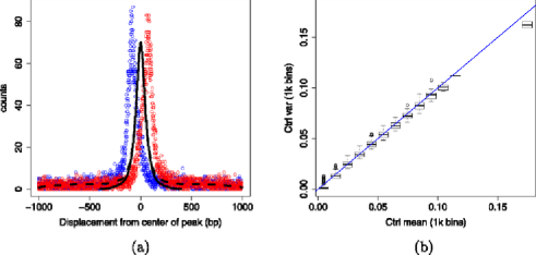
Figure 2: (a) Estimated distribution of tag counts in the forward strand (red) and in the reverse strand (blue) of the FoxA1 data set (chromosome 1). Aligning the distributions and averaging the counts results in the joint count distribution and peak shape (black dashed). The peak shape is multiplied by a quartic biweight function (black solid). (b) Sample mean vs. sample variance of the aligned Control sequence in bins of size 1 Kb. The blue line has slope 1.

2.2 The Poisson model and the STEM algorithm

After alignment, the data consists of a table of genomic locations, each with an associated tag count. The remaining genomic locations are assumed to have a count of zero. Since the data is given as positive integer counts, it is reasonable to model them as Poisson variables [Mikkelsen et al. (2007)]. Specifically, we assume that the IP and Control counts $\operatorname{IP}(t)$ and $\mathrm{C}(t)$ at locations $t$ are independent Poisson sequences

$$\operatorname{IP}(t)\sim\operatorname{Po}\bigl{[}\lambda_{\operatorname{IP}}(t)\bigr{]},\qquad\mathrm{C}(t)\sim\operatorname{Po}\bigl{[}\lambda_{\mathrm{C}}(t)\bigr{]},\qquad t\in\mathbb{Z},$$ (1)

where $\lambda_{\operatorname{IP}}(t)\geq 0$ and $\lambda_{\mathrm{C}}(t)\geq 0$ denote the mean rates at location $t$, which may vary over $t$. The values of the processes $\operatorname{IP}(t)$ and $\mathrm{C}(t)$ are assumed independent over $t$ given $\lambda_{\operatorname{IP}}(t)$ and $\lambda_{\mathrm{C}}(t)$.

As model validation, Figure 2(b) shows a graph of the sample mean vs. sample variance of the aligned Control sequence in the FoxA1 data set, computed in bins of size 1 kbp. The two quantities are nearly proportional with a proportionality constant of 1, as expected from the Poisson model (1). The IP sample exhibits a similar pattern (not shown).

Regions of high binding frequency are represented by peaks in the mean Poisson rates. The goal is to find regions where $\lambda_{\operatorname{IP}}(t)$ is higher than the local background rate $\lambda_{0}(t)$, but also higher than a minimal constant binding rate $\lambda_{\mathrm{L}}$. The lower bound $\lambda_{\mathrm{L}}$ avoids detecting spurious weak peaks in the presence of an even weaker local background. Here $\lambda_{\mathrm{L}}$ is set to the global average rate, equal to the total number of aligned tags in the IP sequence divided by the total length of the genome. Taking the latter as $3.018\times 10^{9}$ [Sakharkar, Chow and Kangueane (2004)], the global average rate for the FoxA1 data set is $\lambda_{\mathrm{L}}=(3.57\times 10^{6})/(3.018\times 10^{9})=0.00118$.

At every $t$, the above comparison translates to testing whether $\lambda_{\operatorname{IP}}(t)\leq\lambda_{0}(t)$ and $\lambda_{\operatorname{IP}}(t)\leq\lambda_{\mathrm{L}}$, that is, $\lambda_{\operatorname{IP}}(t)\leq\max\{\lambda_{0}(t),\lambda_{\mathrm{L}}\}$. To gain efficiency, rather than testing at every single location $t$, tests are performed at only local maxima of the smoothed IP sequence. This is carried out formally using the following adaptation of the STEM algorithm from SGA.

Algorithm 1 ((STEM algorithm)).

[(1)]

Let $w(t)$ be a unimodal kernel of length $W$. Apply kernel smoothing to the IP sequence to produce the smoothed sequence

$$\widetilde{\operatorname{IP}}(t)=w(t)*\operatorname{IP}(t)=\frac{1}{W}\sum_{s=-(W-1)/2}^{(W+1)/2}w(s)\operatorname{IP}(t-s).$$ (2)

Find all local maxima of $\widetilde{\operatorname{IP}}(t)$ as candidate peaks. Let $\tilde{T}$ denote the set of locations of those local maxima.

For each local maximum $t\in\tilde{T}$, compute a $p$-value $p(t)$ for testing the null hypothesis

$$\mathcal{H}_{0}(t)\dvtx\lambda_{\operatorname{IP}}(t)\leq\lambda_{0}^{+}(t)\quad\mbox{vs.}\quad\lambda_{\operatorname{IP}}(t)>\lambda_{0}^{+}(t)$$ (3)

in a neighborhood of $t$, where $\lambda_{0}^{+}(t)=\max\{\lambda_{0}(t),\lambda_{\mathrm{L}}\}$.

Let $\tilde{m}$ be the number of local maxima. Apply a multiple testing procedure on the set of $p$-values and declare significant all peaks whose $p$-values are smaller than the threshold.

Details on each of the steps are given in the following sections.

2.3 Smoothing and local maxima

According to SGA, the best smoothing kernel for the purposes of peak detection is that which maximizes the signal-to-noise ratio (SNR) after convolving the peak shape, assumed to underly the signal peaks in the data, with the smoothing kernel. This is achieved by choosing the smoothing kernel to be equal to the peak shape itself (up to a scaling factor), a principle long known in signal processing as “matched filter theorem” [North (1943), Turin (1960), Pratt (1991), Simon (1995)]. Note that this is not the same as the optimal kernel in nonparametric regression [Wasserman (2006)].

In ChIP-Seq data, binding rate peaks corresponding to different binding sites for the same transcription factor are assumed to have the same shape in terms of spatial spread, but may have different heights. The common peak shape is estimated in the alignment process (solid curve in Figure 2). It is unimodal, constrained to be symmetric, and has heavier tails than the Gaussian density. In Step 1 of the STEM algorithm (Algorithm 1), smoothing was carried out setting $w(t)$ equal to the solid curve in Figure 2, normalized to have unit sum, with $W=801$.

Rows 2 and 3 in Figure 1 compare the raw and smoothed IP data. The smoothed data is high at locations where the density of tag counts is high. Notice that kernel smoothing produces positive counts locations where the unsmoothed IP data may have no counts.

In Step 2 of the STEM algorithm (Algorithm 1), local maxima of the smoothed sequence $\widetilde{\operatorname{IP}}(t)$ are defined as values $\widetilde{\operatorname{IP}}(t)$ that are greater than their immediate neighbors $\widetilde{\operatorname{IP}}(t-1)$ and $\widetilde{\operatorname{IP}}(t+1)$. If the maximum is tied between neighboring values, then the peak location is assigned the lower genomic address. A useful property of the kernel that avoids producing spurious local maxima is to have continuous derivatives. This was ensured by multiplication of the estimated peak shape by a quartic biweight function, as described in Section 2.1 above.

Restricting the analysis to local maxima reduces the amount of data to process further. In the aligned IP sample of the FoxA1 data set, the number of local maxima found was about 2.7 million, down from about 3.9 million original mapped tags.

2.4 Estimation of the local background rate

Computation of $p$-values in Step 3 of the STEM algorithm (Algorithm 1) requires knowledge of the background Poisson rate $\lambda_{0}(t)$ under the null hypothesis. Estimation of $\lambda_{0}(t)$ is difficult because it varies with $t$ in an unknown fashion [Johnson et al. (2007)]. Here we propose a simple method to estimate the background rate from the local Control data, as follows.

Since the Control sample is intended to represent the background process in the IP sample, it is reasonable to assume that the local background rate $\lambda_{0}(t)$ in the IP sample is proportional to the corresponding local background rate $\lambda_{\mathrm{C}}(t)$ in the Control sample, reflecting the ratio in sequencing depth of the background between the two samples. In the FoxA1 data, the IP sample has about 3.9 million tags, while the Control sample has about 5.2 million counts.

The local Control rate $\lambda_{\mathrm{C}}(t)$, in turn, may be estimated as the average tag count in the Control sample within a certain window centered at $t$, as in kernel-based nonparametric regression methods [Wasserman (2006)]. The window size establishes a bias-vs.-variance trade-off in the estimation. While the background rate may change fast, 1 Kb is about the smallest window size that allows comparison of peaks, usually of size a few hundred bp, against the background. Because counts are often sparse, to add stability to the parameter estimates, we consider the local rate to be also linearly related to the corresponding rate in the Control within a window of size 10 Kb centered at $t$.

To illustrate these relationships, Figure 3(a) shows a graph of the 1 Kb bin averages in the Control sample of the FoxA1 data set against the 1 Kb bin averages in the IP sample. While there is a lot of variability, the main trend is seen to be linear, captured in the figure by a marginal linear fit. The outliers in the upper left corner correspond vaguely to the peaks sought. However, their relatively small number introduces little bias in the regression. A similar trend is observed when plotting the 1 Kb bin averages in the IP sample as a function of the 10 Kb bin averages in the Control sample (not shown).

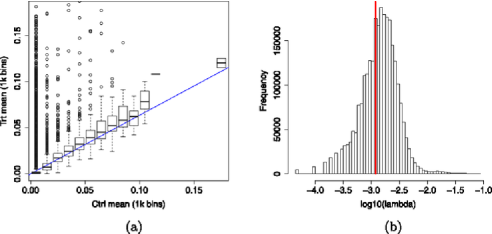
Figure 3: Marginal distributions of the 1 Kb bin averages in the IP sample of the FoxA1 data set as a function of: (a) The 1 Kb bin averages in the Control sample; (b) Histogram of estimated values of $\hat{\lambda}_{0}$ in the FoxA1 data set. As a reference, the global average rate is 0.00118 (red).

Summarizing, $\lambda_{0}(t)$ is estimated from local windows of sizes 1 Kb and 10 Kb centered at $t$ via

$$\hat{\lambda}_{0}(t)=a_{1}\hat{\lambda}_{\mathrm{C},1k}(t)+a_{2}\hat{\lambda}_{\mathrm{C},10k}(t),$$ (4)

where $\hat{\lambda}_{\mathrm{C},1k}(t)$ and $\hat{\lambda}_{\mathrm{C},10k}(t)$ are the Control averages in windows of size 1 Kb and 10 Kb centered at $t$, and $a_{1}$, $a_{2}$ are global parameters. Note that the combination of the 1 Kb and 10 Kb windows plays the role of trapezoidal kernel whose shape is optimally determined by the data-determined coefficients $a_{1}$ and $a_{2}$. To estimate $a_{1}$ and $a_{2}$, we set up a global linear regression as in (4), except that the predictors and the response are replaced by the 1 Kb and 10 Kb bin averages, as in Figure 3(a).

Applying this regression in the FoxA1 data set gave estimates $\hat{a}_{1}=0.307\pm 0.001$ and $\hat{a}_{2}=0.482\pm 0.001$, giving more weight to the 10 Kb window than the 1 kb window. The coefficients automatically account for sequencing depth: if the binding rate in the Control were constant, then the background estimate for the IP would be approximately equal to the Control rate multiplied by the sum of the two window coefficients, equal to 0.789. This factor is slightly smaller than the overall ratio between the total number of aligned counts in the IP sample and in the Control sample, equal to 0.805. The extra counts in the IP sequence are precisely the signal we wish to detect.

The multi-window model makes the estimate adaptive to the local variability in the background rate. As an example, Row 4 of Figure 1 shows the local estimates $\hat{\lambda}_{0}(t)$, roughly following the tag pattern observed in Row 1. Row 5 shows the SNR, defined as the ratio between the peak height $\widetilde{\operatorname{IP}}(t)$ and the estimated background rate $\hat{\lambda}_{0}(t)$. Figure 3(a) shows the distribution of the estimated values of $\hat{\lambda}_{0}(t)$ over the entire genome for the FoxA1 data set.

2.5 Computing $p$-values

In Step 3 of Algorithm 1, the $p$-value $p(t)$ of an observed local maximum of the smoothed sequence $\widetilde{\operatorname{IP}}(t)$ at a location $t$ is defined as the probability to obtain the observed height of the local maximum or higher under the least favorable null hypothesis $\lambda_{\operatorname{IP}}(t)=\lambda_{0}^{+}(t)$ in (3). The null hypothesis need only be assumed in a local neighborhood of each candidate peak because $\widetilde{\operatorname{IP}}(t)$ depends only on the data within a local neighborhood, as dictated by the smoothing kernel $w(t)$. In this section we assume that $\lambda_{0}(t)$ and $\lambda_{\mathrm{L}}$ are known, having been estimated according to the methods described in Section 2.4 above.

In SGA, the background noise process was assumed stationary. In ChIP-Seq data, in contrast, the background rate $\lambda_{0}(t)$ is not constant. However, if the background process is locally stationary, then the background process in the neighborhood of a given location $t=\tilde{t}$ may be assumed to have similar statistical properties in that neighborhood as a stationary sequence with constant background rate $\lambda\equiv\lambda_{0}(\tilde{t})$. In particular, the height of a local maximum of the smoothed sequences at $\tilde{t}$ would have approximately the same distribution in both cases.

Specifically, suppose $X(t;\lambda)$ is a sequence of i.i.d. Poisson random variables with constant mean rate $\lambda$. Smoothing of $X(t;\lambda)$ with the kernel $w(t)$ as in Step 1 of Algorithm 1 produces the smoothed sequence

$$\tilde{X}(t;\lambda)=w(t)*X(t;\lambda)=\frac{1}{W}\sum_{s=-(W-1)/2}^{(W+1)/2}X(t-s;\lambda).$$ (5)

The height of a local maximum of the stationary sequence $\tilde{X}(t;\lambda)$ has the survival function

$$F(u;\lambda)=\mathrm{P}\bigl{[}\tilde{X}(t;\lambda)\geq u|t\mbox{ is a local maximum},\lambda\bigr{]}.$$ (6)

Then, the null distribution of the height of a local maximum of $\widetilde{\operatorname{IP}}(t)$ at $t$ may be approximated by the distribution $F(u;\lambda)$ (6) corresponding to the constant rate $\lambda\equiv\lambda_{0}(t)$. Finally, given the observed height $\widetilde{\operatorname{IP}}(t)$ at $t$, its $p$-value under the null hypothesis (3) is defined as

$$p(t)=F\bigl{(}\widetilde{\operatorname{IP}}(t);\lambda_{0}^{+}(t)\bigr{)}.$$ (7)

The distribution (6) is difficult to compute analytically. Instead, we resort to Monte Carlo simulations, where for each given value of $\lambda$, a long sequence $X(t;\lambda)$ of i.i.d. Poisson variables is generated, smoothed using the kernel $w(t)$, and its local maxima found. The distribution (6) is then estimated empirically from the obtained heights of the local maxima of the smoothed simulated sequence $\tilde{X}(t;\lambda)$ (5).

To reduce computations, rather than performing a new simulation for each new background rate $\lambda_{0}^{+}(t)$, a table of survival functions (6) is prepared in advance for a set of values of $u$ and $\lambda$ that covers the range of possible values to be found in the data. Then, to evaluate $\hat{F}(u;\lambda)$ in (7) for any particular pair of values of $\widetilde{\operatorname{IP}}(t)$ and $\lambda_{0}(t)$, bilinear interpolation is used between the closest grid points.

In the FoxA1 data set, the smallest and largest values of $\hat{\lambda}_{0}(t)$ found were $1.67\times 10^{-5}$ and $7.40\times 10^{-2}$, respectively, giving values of $\hat{\lambda}_{0}^{+}(t)$ in the range 0.00118 to 0.0740. Taking a safety margin of 25%, we performed the Monte Carlo simulation described above for 300 values of $\lambda$ equally spaced on a logarithmic scale between 0.00089 and 0.0925. The length of the simulated Poisson sequences was set to be as long as needed to obtain at least 100 nonzero counts, but not smaller than $1\times 10^{5}$. In order to reduce the variability from the simulation, the table of survival functions $\hat{F}(u,\lambda)$ was smoothed over $\lambda$ for each fixed $u$ via linear regression using 5 B-spline basis functions. The 25% safety margins ensured that none of the values of $\lambda$ actually needed were near the edges of the table for the purposes of spline smoothing.

Figure 4 shows the obtained function $\hat{F}(u;\lambda)$ (6), given as a table of size 300 values of $\lambda$ by 200 values of $u$ and for a few particular values of $\lambda$. As an example, Row 6 of Figure 1 shows the calculated $p$-values $p(t)$ in the corresponding data segments. Because of numerical precision in the Monte Carlo simulations, very low $p$-values could not be distinguished from zero, and in the figures they are drawn as if they were equal to $10^{-10}$.

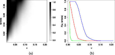
Figure 4: Survival functions $\hat{F}(u;\lambda)$ of the height $u$ of local maxima, approximated by Monte Carlo simulation. (a) Viewed in gray scale as a function of the background rate $\lambda$. (b) Specific survival functions for $\lambda=\lambda_{L}=0.0018$ (green), $\lambda=0.020$ (red), and $\lambda=0.056$ (blue).

Notice in Figure 4 that the smallest value of $u$ is 0.0076, which corresponds to the height of a local maximum obtained from a single tag. Any isolated tag (farther than 1 kb from any other tag) constitutes the smallest possible local maximum and thus gets a $p$-value of 1 regardless of the estimated background rate. In this sense, using the global average rate $\lambda_{L}=0.00118$, corresponding to about 1 tag per 1 Kb, as an absolute reference, is not restrictive. However, the results are sensitive to the choice of $\lambda_{L}$ in the sense that, if $\lambda_{L}$ is larger than the estimated background rate $\lambda_{0}(t)$ at any location $t$, then $\lambda_{0}^{+}(t)=\lambda_{L}$ is used as the rate for the null hypothesis rather than the estimated local background rate $\lambda_{0}$. This can affect the significance of stronger peaks and it is therefore preferable to choose a value of $\lambda_{L}$ that is not large, as it is done here.

2.6 Multiple testing

Following SGA, we applied the BH procedure on the sequence of $\tilde{m}=2\mbox{,}643\mbox{,}095$ $p$-values from the FoxA1 data set, each corresponding to a local maximum of the smoothed sequence $\widetilde{\operatorname{IP}}(t)$. Of these local maxima, 21,986 were declared significant at an FDR level of 0.01. Their associated addresses $t$ are effectively point estimates of the locations of the binding sites they represent.

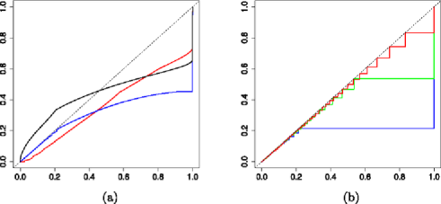
Figure 5: Marginal distribution of $p$-values in the FoxA1 data set: (a) observed (black) and estimated under the global null hypothesis empirically (red) and theoretically (blue); (b) specific null distributions for $\lambda=0.0012$ (blue), $\lambda=\lambda_{\mathrm{L}}=0.0018$ (green), and $\lambda=0.0030$ (red).

As an example, in Row 3 of Figure 1, the significant local maxima are indicated by red circles. As final results, the detected peaks were ranked according to their $p$-values. Of the 21,986 significant peaks, the top 7284 had $p$-values that could not be distinguished from 0 because of the numerical accuracy of our Monte Carlo simulations. These peaks were ranked according to their SNR.

To assess the validity of the procedure, Figure 5(a) compares the observed marginal distribution of $p$-values to the expected marginal distribution under the complete null hypothesis in the FoxA1 data set. The observed marginal distribution of $p$-values [shown in black in Figure 5(a)] is given by the empirical distribution

$$\hat{G}(p)=\frac{1}{\tilde{m}}\sum_{t\in\tilde{T}}\mathbf{1}\bigl{[}p(t)\leq p\bigr{]},\qquad 0\leq p\leq 1,$$ (8)

where $\tilde{T}$ is the set of $\tilde{m}$ locations of the local maxima of $\widetilde{\operatorname{IP}}(t)$, with $p$-values given by (7). The marginal distribution under the complete null hypothesis is estimated in two different ways, one purely empirical and one more theoretical.

The empirical estimate [shown in red in Figure 5(a)] was obtained by running the entire analysis on the Control sample as if it were the IP, that is, searching for peaks in the Control sample using the same Control sample for estimating the background. The obtained null distribution of $p$-values lies below the diagonal as required for validity, and it exhibits a high frequency of $p$-values equal to 1, corresponding to peaks with only one tag in them.

The theoretical estimate [shown in blue in Figure 5(a)] was obtained as follows. Recall that for a smoothed stationary Poisson sequence $\tilde{X}(t;\lambda)$ with constant rate $\lambda$, the distribution of the height of a local maximum at $t\in\tilde{T}$ is given by (6). Analogous to (7), define the corresponding null $p$-value as $p_{0}(t)=F(\tilde{X}(t);\lambda)$ for $t\in\tilde{T}$. Its distribution $G_{0}(p;\lambda)=P(p_{0}(t)\leq p)$ for any $t$ is given by

$$G_{0}(p;\lambda)=\cases{1,&\quad$F(u_{1};\lambda)\leq p$,\vspace*{2pt}\cr F(u_{k};\lambda),&\quad$F(u_{k};\lambda)\leq p<F(u_{k-1};\lambda),k=2,3,\ldots,$}$$ (9)

where $u_{k}$, $k=1,2,\ldots,$ are the discrete values taken by the smoothed process $\tilde{X}(t;\lambda)$ at the local maxima. Note that $G_{0}(p;\lambda)$ is independent of $t$ for $t\in\tilde{T}$ because of stationarity. In the ChIP-Seq problem, we approximate the null distribution of the $p$-value at $t\in\tilde{T}$ by the null distribution $G_{0}(p;\hat{\lambda}_{0}^{+}(t))$ corresponding to a stationary process with constant rate $\lambda=\hat{\lambda}_{0}(t)$, which depends on $t$ only through the value of $\lambda$. Since each of the observed $p$-values in (8) corresponds to a different background rate $\hat{\lambda}_{0}(t)$, the estimated marginal distribution under the global null hypothesis is given by the mixture distribution

$$\hat{G}_{0}(p)=\frac{1}{\tilde{m}}\sum_{t\in\tilde{T}}G_{0}\bigl{(}p;\hat{\lambda}^{+}_{0}(t)\bigr{)},\qquad 0\leq p\leq 1.$$ (10)

Referring back to Figure 5(a), the observed distribution is always above the null distribution, and the large derivative at zero indicates the presence of a strong signal, which explains the large number of significant peaks found. Note that the null distribution is not uniform but stochastically larger. To better understand the mixture (10), Figure 5(b) shows three examples of the individual null distributions (9). All are discrete and stochastically larger than the continuous uniform distribution. For small $\lambda$, the most common $p$-value is 1, as most local maxima take the smallest possible value $u_{1}$, equal to the mode of the kernel $w(t)$, obtained when there is an isolated count of 1 in a neighborhood of zeros. This explains the large jump at 1 in panel (a). As $\lambda$ gets larger, the distribution becomes closer to the continuous uniform distribution.

3 Comparison to other methods

As a reference, we compared our method to MACS, cisGenome and QuEST on both the FoxA1 and GABP data sets. While the FoxA1 data set was used in the development of MACS and our method, the GABP data set was not used in the development of any of the three methods, providing an independent test of performance. All methods were applied using the default values and an FDR cutoff of 0.01. Table 1 indicates the number of significant peaks obtained in each case. The methods are compared by a motif analysis and in terms of their mutual agreement below.

Table 1: Number of significant peaks called by all methods at FDR level 0.01

Dataset	STEM${}\bolds{+}{}$Regr	MACS	cisGenome	QuEST
FoxA1	21,986	13,639	5725	20,161
GABP	.03309	13,828	4275	0.6442

3.1 Motif analysis

As biological validation, a motif analysis was performed where, for each peak declared significant, the number of motifs related to the appropriate transcription factor was counted within 100 bp and 400 bp of the estimated peak location. The distance of 400 bp approximately corresponds to the spatial spread of the measurements belonging to a binding site, as determined by the estimate in Figure 2(a).

Table 2 shows the average number of motifs and the proportion of peaks with at least one motif within those distances for the top 5725 peaks found by each method in the FoxA1 data set and the top 3309 peaks found by each method in the GABP data set. These numbers are the minima of the rows in Table 1. Taking the same number of top peaks in each list makes the averages and proportions in the table comparable, as the peak lists are ordered and the various methods use different criteria for their list cutoffs. Our method, labeled “STEM${}+{}$Regr” for simplicity, shows a similar performance to the other methods. Given the standard errors, it is difficult to claim superiority of any method over the others.

Table 2: Motif analysis comparing the performance of the proposed method against MACS and cisGenome on two different data sets. Results are for the top 5725 peaks in each method for the FoxA1 data set and the top 3309 peaks in each method for the GABP data set. Standard errors are all between 1% and 2% of the number shown

		Average number of		Proportion with at
		motifs within		least one motif within
Dataset	Method	100 bp	400 bp	100 bp	400 bp
FoxA1	STEM${}+{}$Regr	0.916	1.868	0.623	0.837
	MACS	0.917	1.849	0.625	0.835
	cisGenome	0.915	1.833	0.619	0.830
	QuEST	0.844	1.784	0.576	0.816
GABP	STEM${}+{}$Regr	0.880	1.708	0.573	0.788
	MACS	0.875	1.703	0.579	0.792
	cisGenome	0.862	1.658	0.562	0.766
	QuEST	0.868	1.725	0.578	0.804

3.2 Peak overlap and discrepancies

To help explain the previous results, Table 3 compares the percentage of peaks from the top 5725 from each method in the FoxA1 data set or the top 3309 from each method in the GABP data set, that were also found by each of the other methods within a distance of 100 bp and 400 bp. The matrices in the table are not symmetric because the correspondence between peaks is not one-to-one; peaks found by one method may be represented by two or more peaks found by another method. The table shows that there is a fair amount of overlap between the methods, particularly in the GABP data set where the peak lists are smaller (Table 1).

Table 3: Percentage of peaks from the methods listed in the columns that were also found by the methods listed in the rows within a distance of 100 bp and 400 bp.Results are for the top 5725 peaks from each method in the FoxA1 data setand the top 3309 peaks from each method in the GABP data set

		% found within 100 bp				% found within 400 bp
Dataset	Method	STEM${}\bolds{+}{}$Regr	MACS	cisGenome	QuEST	STEM${}\bolds{+}{}$Regr	MACS	cisGenome	QuEST
FoxA1	STEM${}+{}$Regr	$100$	$81.0$	$76.8$	$64.1$	$100$	$84.4$	$79.5$	$64.5$
	MACS	$79.6$	$100$	$84.4$	$70.8$	$80.1$	$100$	$84.9$	$71.0$
	cisGenome	$75.1$	$84.4$	$100$	$68.8$	$75.4$	$84.9$	$100$	$68.8$
	QuEST	$64.2$	$71.5$	$70.5$	$100$	$69.3$	$80.5$	$77.9$	$100$
GABP	STEM${}+{}$Regr	$100$	$90.1$	$83.7$	$89.8$	$100$	$92.8$	$86.5$	$89.9$
	MACS	$90.1$	$100$	$84.7$	$87.8$	$90.4$	$100$	$85.8$	$87.9$
	cisGenome	$83.7$	$84.7$	$100$	$80.8$	$84.1$	$85.8$	$100$	$80.8$
	QuEST	$90.1$	$87.8$	$80.8$	$100$	$93.9$	$94.1$	$86.7$	$100$

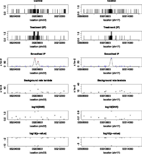
Figure 6: Left: A fragment of the aligned GABP data featuring a secondary peak called by our method but not MACS or cisGenome. Right: A fragment of the aligned GABP data featuring a peak called by MACS and cisGenome but not by our method. The variables plotted are the same as in Figure 1. Notice the difference in vertical scales between the left and right panels.

To better understand the discrepancies, Figure 6 shows two examples of genomic segments from the GABP data set after alignment. The left panel shows one of the 32 peaks produced by our method that were not found among the peaks produced by MACS or cisGenome. Our method detected a secondary peak within 567 bp of a major peak (Row 3), in a binding region that was counted as a single region by both MACS and cisGenome. All the other peaks in this group of 32 were found to be secondary peaks or sometimes tertiary peaks, with distances between 385 bp and 1113 bp from their closest neighbor.

These secondary peaks, not distinguished by MACS or cisGenome, may be separate binding sites. The ability to resolve them is a consequence of our method searching for binding sites rather than binding regions. These secondary sites were also found by QuEST, but were often represented by perhaps too many peaks. For example, the secondary peak in the left panel of Figure 6 was identified by QuEST as two peaks, but being within only 131 bp of each other, they may not belong to separate sites. The ability to represent a single site by a single peak is a consequence of our method using a matched filter rather than a narrow Gaussian filter.

The right panel of Figure 6 shows one of the 575 of the peaks that were produced by MACS and called by cis Genome and QuEST but were not among the top 3309 produced by our method. This peak was not called significant by our method because its associated $p$-value was not low enough (Row 6). This is because the peak height is low (Row 3), while the estimated local background rate is high (Row 4), resulting in a relatively low SNR (Row 5). Other peaks in this group of 575 were similar. This example illustrates the importance of the estimation of the local background rate in the analysis.

4 Simulations

In order to evaluate the accuracy of the background rate estimation method and the performance of the STEM algorithm for peak detection, we performed the following spike-in simulated experiment. In each simulated data set, two independent Poisson sequences of length $L=10^{7}$ base pairs representing an aligned IP sequence and an aligned control sequence were generated according to model (1). The control background rate $\lambda_{\mathrm{C}}(t)$ was obtained from chromosome 2 of the FoxA1 data set in a way similar to model (4) as

$$\lambda_{\mathrm{C}}(t)=a_{1}\hat{\lambda}_{\mathrm{C},1k}(t)+a_{2}\hat{\lambda}_{\mathrm{C},10k}(t),$$

where $\hat{\lambda}_{\mathrm{C},1k}(t)$ and $\hat{\lambda}_{\mathrm{C},10k}(t)$ are the Control averages in windows of size 1 Kb and 10 Kb centered at $t$, $a_{1}=0.3$ and $a_{2}=0.7$. To simulate a different enrichment between the IP and control sequences, the IP background rate was set to $\lambda_{0}(t)=0.8\lambda_{C}(t)$. Then the actual IP rate was set to $\lambda_{IP}(t)=\lambda_{0}(t)+S\lambda^{+}(t)$, where $\lambda^{+}(t)$ is a sequence of 20 spikes with shape equal to the solid curve in Figure 2 but normalized so that the area under each peak is equal to the mean of $\lambda_{0}(t)$. Because of this normalization, the factor $S$ can be interpreted as the signal-to-noise ratio and it was set to values between 5 and 15.

Figure 7(a) shows the realized FDR and detection power (defined as the fraction of detected peaks) averaged over 10 independent data sets simulated as described above. The proposed STEM${}+{}$Regr algorithm shows similar performance and error control as cisGenome. MACS’s apparent low power may be rather an indication that the algorithm is not intended to be applied to short sequences like the ones used in this simulated experiment. Results for QuEST were not obtained because the need for user input makes the software not conducive for repeated simulation experiments of this kind.

Figure 7: Spike-in simulated experiment in a section of Chromosome 2. (a) Detection performance of the three methods: STEM${}+{}$Regr (red), cisGenome (blue) and MACS (green). Detection power is shown with solid lines, FDR with dotted lines. Black dashed line is the nominal FDR level 0.1. (b) Estimation of the background rate $\lambda_{0}(t)$ as a function of genomic location $t$ (selected fragment): simulated (black) and estimated (red).

Looking closer at the regression method for estimating the background rate $\lambda_{0}(t)$, Figure 7(b) shows that the regression method is able to follow the general trend of the local background rate despite it varying quickly. To reduce variability, the method automatically performs a bias-variance trade-off, where the coefficients $C\times a_{1}=0.24$ and $C\times a_{2}=0.56$ are estimated on average as 0.096 and 0.678, respectively. The overall correlation between the simulated and predicted background rate is 0.73.

5 Discussion

5.1 Methodological considerations

We have presented a method for detection of peaks in ChIP-Seq data based on the STEM algorithm of SGA with promising results. The applicability of SGA to ChIP-Seq data relied on the common assumption that the signal peaks, represented by a mean function, are unimodal and have the same shape up to an amplitude scaling factor. The adaptation to ChIP-Seq data required two main modifications: (1) estimation of the local background rate; (2) use of Monte Carlo simulations of Poisson sequences to compute $p$-values.

From a methodological point of view, estimation of the background rate $\lambda_{0}(t)$ is arguably the most crucial step in the analysis, as the inference for a particular local maximum is highly dependent on the background rate at that location. In this paper, we have focused on the inference aspects of detecting peaks with a spatial structure via the STEM algorithm. Estimation of the local background rate (the particle “Regr” in the acronym “STEM${}+{}$Regr”) is not part of the original STEM algorithm, but is necessary for the analysis of ChIP-Seq data because the noise process is not stationary. This conceptual separation is helpful in that the background estimation method could be replaced by a different method if desired, without affecting the general implementation of the STEM algorithm for peak detection.

Statistical methods for estimating the variable rate $\lambda(t)$ in dynamic Poisson models or nonhomogeneous Poisson sequences have been developed in other contexts. Bayesian methods [West, Harrison and Migon (1985), Harvey and Durbin (1986), Bolstad (1995)] are computationally intensive, estimating $\lambda(t)$ at each location $t$ based on the estimates at locations $1,2,\ldots,t-1$. This is computationally infeasible for long genomic sequences as in ChIP-Seq data. Other methods require either repeated realizations [Arkin and Leenis (2000)] or a more specific structure of the process [Zhao and Xie (1996), Helmers, Mangku and Zitikis (2003)], which are not available in ChIP-Seq data.

In this paper we have proposed a simple solution to local background estimation based on multiple linear regression using the Control sample as a covariate. If desired, other covariates could be included such as other window sizes and the local GC content. Estimating the regression coefficients from the data automatically adjusts for sequencing depth, and the estimated relative weighting between the various window sizes allows the method to adaptively estimate the local background at each location. In this sense, the regression model solves the normalization problem and gives a partial answer to the question of how slowly $\lambda_{0}(t)$ varies with $t$. Because the GABP data set is richer in number of reads, the regression method automatically accounts for it and allows estimation of the background rate at a smaller spatial scale by giving a higher weight to the 1 kb window relative to the 10 kb window than in the FoxA1 data set.

Often in ChIP-Seq data a Control sample is unavailable. In such cases, the regression model (4) could have the 10 Kb averages from the IP sample itself as predictors instead of those from the Control, with the 1 Kb window not included in the model. This would allow estimation of the background from the neighborhood of each peak, albeit with some positive bias. Fortunately, the positive bias would make the inference more conservative, affecting the detection power more than its validity.

In the comparison with the other methods, it was observed that the STEM algorithm performs competitively in terms of nearby motifs. In the data sets analyzed, all methods found many of the same strong peaks. However, our method found secondary and terciary peaks near other strong peaks that were not distinguished by MACS and cisGenome and were too fragmented by QuEST. This is a result of our method searching for localized binding sites using an appropriately chosen matched filter rather than binding regions of arbitrary size.

On the other hand, our method did not call significant other peaks that were called by the other methods. These peaks were not strong enough when compared to their corresponding background estimate at that location, at least according to the background estimation method used here. It is possible that a different background estimation method would have caused these peaks to be called significant. In fact, the other methods did because they had different assumptions about what represents a strong peak.

In this paper, we have attempted to frame the ChIP-Seq problem as a formal multiple testing problem. The significance results and FDR levels may be trusted under the proposed model, however, the biological validity of the results is limited by the validity of the modeling assumptions. Particularly difficult is the background estimation, for which no good model exists to date. Because of its importance, background estimation is where future research in ChIP-Seq analysis should focus its attention.

5.2 Computational considerations

In addition to the modelling considerations mentioned above, the final ranking of the detected peaks depends on the numerical accuracy with which $p$-values are computed. In the Monte Carlo simulations for computing the distribution of the heights of local maxima, the estimation is more accurate for high values of $\lambda$, as these produce more observations. In the simulations, we set the simulation length to be at least $10^{5}$, or as long as is needed to obtain at least 100 Poisson counts. The latter condition was necessary for very low Poisson rates, but cannot be considered sufficient. The random variability was attenuated by B-spline smoothing across $\lambda$ in order to obtain the table in Figure 4(b).

In the analysis results, we observed that a large number of detected peaks had a $p$-value of zero, meaning that the Monte Carlo simulation did not have enough numerical resolution to distinguish between their $p$-values. These peaks were ranked sub-optimally by SNR. More accurate calculation of $p$-values could be achieved with longer Monte Carlo simulations or by more sophisticated simulation techniques, such as Importance Sampling.

Computational complexity is also important in ChIP-Seq analysis because of the large amount of data to be processed. The methods in this paper were implemented in R to ease their development and sharing among researchers, but at the expense of computational speed. The main computational bottleneck of our method is kernel smoothing, taking about $6\sim 8$ hours to run over the entire genome on a Dell Power Edge R710 server with CPU speed 2.67 GHz, 48 GB of memory and a Linux CentOS 5.5 operating system. All the other processing steps together take about another hour. Kernel smoothing is mathematically simple, yet unfortunately inefficient in R for very long sequences. Computing time for kernel smoothing increases linearly with the kernel and the sequence size. In our implementation, the data was divided into subgroups of tags no more than $10^{4}$ bp apart, trading off the length of the groups and their number. Computational time was also reduced by reducing the length of the kernel by multiplying it by a quartic biweight function of smaller support and using run length encoding in the search for local maxima. In the future the ideas proposed here could be made computationally competitive by implementing them in C.

We do not intend that the method proposed in this paper is viewed as a competitor to other existing methods for analyzing ChIP-Seq data, but rather as a suggestion of how multiple testing theory for spatial domains, such as in SGA, can inform the inference procedure in the detection of peaks. While competitive in terms of detection performance, the strength of our method relies mainly on the potential generalization of these ideas to other domains in spatial inference, both in bioinformatics and beyond.

Appendix: Alignment details

.3 Raw data

The FoxA1 raw data consists of a table of about 3.9 million rows for the IP sample and a table of about 5.2 million rows for the Control sample. Each row corresponds to a mapped tag of length 35 bp and contains the beginning and end genomic addresses for the tag and an indicator of whether the tag belongs to the forward ($+$) or reverse ($-$) DNA strand. We define the location of a tag to be given by its beginning address, corresponding to the lower address for the forward ($+$) tags and the higher address for the reverse ($-$) tags. The GABP data set, containing about 7.8 million tags in the IP sample and about 17.4 million tags in the Control sample, was converted to the same format before processing. Genomic locations not listed in the table were assumed to have an associated tag count of zero. Duplicate tags were considered measurement artifacts and were removed from the analysis.

In order to be counted together, the tags from the two strands need to be aligned with each other. We followed an alignment method similar to that in MACS, shifting all tags by the same amount in the 3’ direction of the tag sequence toward the most likely binding site: forward $(+)$ tags toward higher genomic addresses and reverse $(-)$ tags toward lower genomic addresses. Once shifted, tags coinciding at the same location are counted together. The result of this process is a table of genomic locations, each with an associated tag count. This aligned data is used as the input for peak detection, described in Section 2.

.4 Estimation of the tag shift and peak shape

As in MACS, we estimate the size of the shift from the tag count distributions corresponding to a set of strong and easily detectable peaks, as described below. We performed the shift estimation on Chromosome 1 because of its likelihood to contain enough such strong peaks, but other long chromosomes could be used instead. As part of the process, the shift estimation also allows us to estimate the distribution of shifted tags counts around a peak. This peak shape, normalized to unit sum, is used later as a smoothing kernel in the STEM algorithm for peak detection. The estimation proceeds as follows.

Algorithm 2 ((Estimation of shift size and peak shape)).

[(1)]

Temporarily shift all tags [$(+)$ forward and $(-)$ back] by a tentative shift amount (default 100 bp). This produces a table of genomic locations, each with an associated tag count.

Perform peak detection on the count data from the previous step and select a set of strong peaks (details given below). Let $t_{1},\ldots,t_{N}$ be their locations.

Set a window size $W$ (an odd number, default 2001 bp). The distribution of the forward tags is a vector of length $W$ whose $i$th entry is equal to the average number of forward tags at a constant distance $(W+1)/2-i$ from the peak, that is, at locations $t_{j}-(W+1)/2+i$, $j=1,\ldots,N$. Repeat for the reverse tags.

Fit a spline to the distribution of forward tags and record its mode. Repeat for the reverse tags. The estimated shift is half the distance between the two modes, rounded to the nearest integer.

To estimate the peak shape, shift the original forward and reverse distributions by the estimated shift, symmetrize the joint distribution by averaging both the forward and reverse tag distributions and their mirror images with respect to the center of the window, and fit a spline.

The peak detection step (Step 2) above need not be exact. Since the tag distribution is evaluated in a window around the strong peaks, it is enough that the true location of those peaks is contained somewhere near the center of that window. To achieve this, we apply the first half of the STEM algorithm, as follows. [(2a)]

Set a tentative unimodal symmetric kernel (default Gaussian with standard deviation 50) and perform kernel smoothing on the count data from Step 1. (Implementation details given in Section 2.3).

Find the local maxima of the smoothed count sequence. (Implementation details given in Section 2.3).

Select the $N$ highest local maxima (default 1000).

At the end of this process, the data consists of a long sequence of genomic addresses and associated counts 0, 1 or 2, ready for peak detection analysis. The maximal count of 2 is a result of the elimination of duplicates from the original list of tags. Because binding rates are generally low, truncation at 2 does not greatly affect the Poisson model used thereafter.

References

- Arkin and Leenis (2000) {barticle}[author] \bauthor\bsnmArkin, \bfnmBradford L.\binitsB. L. and \bauthor\bsnmLeenis, \bfnmLawrence M.\binitsL. M. (\byear2000). \btitleNonparametric estimation of the cumulative intensity function for a nonhomogeneous Poisson process from overlapping realizations. \bjournalManagement Science \bvolume46 \bpages989–998. \bptokimsref \endbibitem
- Barski and Zhao (2009) {barticle}[pbm] \bauthor\bsnmBarski, \bfnmArtem\binitsA. and \bauthor\bsnmZhao, \bfnmKeji\binitsK. (\byear2009). \btitleGenomic location analysis by ChIP-Seq. \bjournalJ. Cell. Biochem. \bvolume107 \bpages11–18. \biddoi=10.1002/jcb.22077, issn=1097-4644, pmid=19173299 \bptokimsref \endbibitem
- Benjamini and Hochberg (1995) {barticle}[mr] \bauthor\bsnmBenjamini, \bfnmYoav\binitsY. and \bauthor\bsnmHochberg, \bfnmYosef\binitsY. (\byear1995). \btitleControlling the false discovery rate: A practical and powerful approach to multiple testing. \bjournalJ. Roy. Statist. Soc. Ser. B \bvolume57 \bpages289–300. \bidissn=0035-9246, mr=1325392 \bptokimsref \endbibitem
- Bolstad (1995) {barticle}[mr] \bauthor\bsnmBolstad, \bfnmWilliam M.\binitsW. M. (\byear1995). \btitleThe multiprocess dynamic Poisson model. \bjournalJ. Amer. Statist. Assoc. \bvolume90 \bpages227–232. \bidissn=0162-1459, mr=1325130 \bptokimsref \endbibitem
- Fejes et al. (2008) {barticle}[author] \bauthor\bsnmFejes, \bfnmA.\binitsA., \bauthor\bsnmRobertson, \bfnmG.\binitsG., \bauthor\bsnmBilenky, \bfnmM.\binitsM., \bauthor\bsnmVarhol, \bfnmR.\binitsR., \bauthor\bsnmBainbridge, \bfnmM.\binitsM. and \bauthor\bsnmJones, \bfnmS.\binitsS. (\byear2008). \btitleFindPeaks 3.1: A tool for identifying areas of enrichment from massively parallel short-read sequencing technology. \bjournalBioinformatics \bvolume24 \bpages1720–1730. \bptokimsref \endbibitem
- Harvey and Durbin (1986) {barticle}[author] \bauthor\bsnmHarvey, \bfnmA. C.\binitsA. C. and \bauthor\bsnmDurbin, \bfnmJ.\binitsJ. (\byear1986). \btitleThe effects of seat belt legislation on British road casualties: A case study in structural time series modelling. \bjournalJ. Roy. Statist. Soc. \bvolume149 \bpages187–227. \bptokimsref \endbibitem
- Helmers, Mangku and Zitikis (2003) {barticle}[mr] \bauthor\bsnmHelmers, \bfnmRoelof\binitsR., \bauthor\bsnmMangku, \bfnmI. Wayan\binitsI. W. and \bauthor\bsnmZitikis, \bfnmRičardas\binitsR. (\byear2003). \btitleConsistent estimation of the intensity function of a cyclic Poisson process. \bjournalJ. Multivariate Anal. \bvolume84 \bpages19–39. \biddoi=10.1016/S0047-259X(02)00008-8, issn=0047-259X, mr=1965821 \bptokimsref \endbibitem
- Hower, Evans and Pachter (2011) {barticle}[author] \bauthor\bsnmHower, \bfnmValerie\binitsV., \bauthor\bsnmEvans, \bfnmSteve N.\binitsS. N. and \bauthor\bsnmPachter, \bfnmLior\binitsL. (\byear2011). \btitleShape-based identification for ChIP-Seq. \bjournalBMC Bioinformatics \bvolume12 \bpages15. \bptokimsref \endbibitem
- Jaffe et al. (2012) {barticle}[pbm] \bauthor\bsnmJaffe, \bfnmAndrew E.\binitsA. E., \bauthor\bsnmFeinberg, \bfnmAndrew P.\binitsA. P., \bauthor\bsnmIrizarry, \bfnmRafael A.\binitsR. A. and \bauthor\bsnmLeek, \bfnmJeffrey T.\binitsJ. T. (\byear2012). \btitleSignificance analysis and statistical dissection of variably methylated regions. \bjournalBiostatistics \bvolume13 \bpages166–178. \biddoi=10.1093/biostatistics/kxr013, issn=1468-4357, pii=kxr013, pmcid=3276267, pmid=21685414 \bptokimsref \endbibitem
- Ji et al. (2008) {barticle}[author] \bauthor\bsnmJi, \bfnmHongkai\binitsH., \bauthor\bsnmJiang, \bfnmHui\binitsH., \bauthor\bsnmMa, \bfnmWenxiu\binitsW., \bauthor\bsnmJohnson, \bfnmDavid S.\binitsD. S., \bauthor\bsnmMyers, \bfnmRichard M.\binitsR. M. and \bauthor\bsnmWong, \bfnmWing H.\binitsW. H. (\byear2008). \btitleAn integrated software system for analyzing ChIP-chip and ChIP-Seq data. \bjournalNature Biotechnology \bvolume26 \bpages1293–1300. \bptokimsref \endbibitem
- Johnson et al. (2007) {barticle}[pbm] \bauthor\bsnmJohnson, \bfnmDavid S.\binitsD. S., \bauthor\bsnmMortazavi, \bfnmAli\binitsA., \bauthor\bsnmMyers, \bfnmRichard M.\binitsR. M. and \bauthor\bsnmWold, \bfnmBarbara\binitsB. (\byear2007). \btitleGenome-wide mapping of in vivo protein-DNA interactions. \bjournalScience \bvolume316 \bpages1497–1502. \biddoi=10.1126/science.1141319, issn=1095-9203, pii=1141319, pmid=17540862 \bptokimsref \endbibitem
- Mikkelsen et al. (2007) {barticle}[author] \bauthor\bsnmMikkelsen, \bfnmT. S.\binitsT. S., \bauthor\bsnmKu, \bfnmM.\binitsM., \bauthor\bsnmJaffe, \bfnmD. B.\binitsD. B., \bauthor\bsnmIssac, \bfnmB.\binitsB., \bauthor\bsnmLieberman, \bfnmE.\binitsE., \bauthor\bsnmGiannoukos, \bfnmG.\binitsG., \bauthor\bsnmAlvarez, \bfnmP.\binitsP., \bauthor\bsnmBrockman, \bfnmW.\binitsW., \bauthor\bsnmKim, \bfnmT. K.\binitsT. K., \bauthor\bsnmKoche, \bfnmR. P.\binitsR. P., \bauthor\bsnmLee, \bfnmW.\binitsW., \bauthor\bsnmMendenhall, \bfnmE.\binitsE., \bauthor\bsnmO’Donovan, \bfnmA.\binitsA., \bauthor\bsnmPresser, \bfnmA.\binitsA., \bauthor\bsnmRuss, \bfnmC.\binitsC., \bauthor\bsnmXie, \bfnmX.\binitsX., \bauthor\bsnmMeissner, \bfnmA.\binitsA., \bauthor\bsnmWernig, \bfnmM.\binitsM., \bauthor\bsnmJaenisch, \bfnmR.\binitsR., \bauthor\bsnmNusbaum, \bfnmC.\binitsC., \bauthor\bsnmLander, \bfnmE. S.\binitsE. S. and \bauthor\bsnmBernstein, \bfnmB. E.\binitsB. E. (\byear2007). \btitleGenome-wide maps of chromatin state in pluripotent and lineage-committed cells. \bjournalNature \bvolume448 \bpages553–560. \bptokimsref \endbibitem
- North (1943) {bmisc}[author] \bauthor\bsnmNorth, \bfnmD. O.\binitsD. O. (\byear1943). \bhowpublishedAn analysis of the factors which determine signal/noise discrimination in pulsed carrier systems. Technical Report No. PTR-6C, RCA Labs, Princeton, NJ. \bptokimsref \endbibitem
- Park (2009) {barticle}[pbm] \bauthor\bsnmPark, \bfnmPeter J.\binitsP. J. (\byear2009). \btitleChIP-seq: Advantages and challenges of a maturing technology. \bjournalNat. Rev. Genet. \bvolume10 \bpages669–680. \biddoi=10.1038/nrg2641, issn=1471-0064, mid=NIHMS327265, pii=nrg2641, pmcid=3191340, pmid=19736561 \bptokimsref \endbibitem
- Pratt (1991) {bbook}[author] \bauthor\bsnmPratt, \bfnmWilliam K.\binitsW. K. (\byear1991). \btitleDigital Image Processing. \bpublisherWiley, \blocationNew York. \bptokimsref \endbibitem
- Sakharkar, Chow and Kangueane (2004) {barticle}[author] \bauthor\bsnmSakharkar, \bfnmMeena Kishore\binitsM. K., \bauthor\bsnmChow, \bfnmVincent T. K.\binitsV. T. K. and \bauthor\bsnmKangueane, \bfnmPandjassarame\binitsP. (\byear2004). \btitleDistributions of exons and introns in the human genome. \bjournalIn Silico Biology \bvolume4 \bpages0032. \bptokimsref \endbibitem
- Schwartzman, Gavrilov and Adler (2011) {barticle}[author] \bauthor\bsnmSchwartzman, \bfnmArmin\binitsA., \bauthor\bsnmGavrilov, \bfnmYulia\binitsY. and \bauthor\bsnmAdler, \bfnmRobert J.\binitsR. J. (\byear2011). \btitleMultiple testing of local maxima for detection of peaks in 1D. \bjournalAnn. Statist. \bvolume39 \bpages3290–3319. \bidmr=3012409 \bptokimsref \endbibitem
- Simon (1995) {bbook}[author] \bauthor\bsnmSimon, \bfnmMarvin\binitsM. (\byear1995). \btitleDigital Communication Techniques: Signal Design and Detection. \bpublisherPrentice Hall, \blocationEnglewood Cliffs, NJ. \bptokimsref \endbibitem
- Spyrou et al. (2009) {barticle}[author] \bauthor\bsnmSpyrou, \bfnmC.\binitsC., \bauthor\bsnmStark., \bfnmR.\binitsR., \bauthor\bsnmLynch, \bfnmA. G.\binitsA. G. and \bauthor\bsnmTavar, \bfnmS.\binitsS. (\byear2009). \btitleBayesian analysis of ChIP-Seq data. \bjournalBMC Bioinformatics \bvolume10 \bpages299. \bptokimsref \endbibitem
- Turin (1960) {barticle}[mr] \bauthor\bsnmTurin, \bfnmGeorge L.\binitsG. L. (\byear1960). \btitleAn introduction to matched filters. \bjournalTrans. IRE \bvolumeIT-6 \bpages311–329. \bidmr=0115847 \bptokimsref \endbibitem
- Valouev et al. (2008) {barticle}[author] \bauthor\bsnmValouev, \bfnmA.\binitsA., \bauthor\bsnmJohnson, \bfnmD. S.\binitsD. S., \bauthor\bsnmSundquist, \bfnmA.\binitsA., \bauthor\bsnmMedina, \bfnmC.\binitsC., \bauthor\bsnmAnton, \bfnmE.\binitsE., \bauthor\bsnmBatzglou, \bfnmS.\binitsS., \bauthor\bsnmMyers, \bfnmR. M.\binitsR. M. and \bauthor\bsnmSidow, \bfnmA.\binitsA. (\byear2008). \btitleGenome-wide analysis of transcription factor binding sites based on ChIP-Seq data. \bjournalNature Methods \bvolume5 \bpages829–834. \bptokimsref \endbibitem
- Wasserman (2006) {bbook}[mr] \bauthor\bsnmWasserman, \bfnmLarry\binitsL. (\byear2006). \btitleAll of Nonparametric Statistics. \bpublisherSpringer, \blocationNew York. \bidmr=2172729 \bptokimsref \endbibitem
- West, Harrison and Migon (1985) {barticle}[mr] \bauthor\bsnmWest, \bfnmMike\binitsM., \bauthor\bsnmHarrison, \bfnmP. Jeff\binitsP. J. and \bauthor\bsnmMigon, \bfnmHélio S.\binitsH. S. (\byear1985). \btitleDynamic generalized linear models and Bayesian forecasting. \bjournalJ. Amer. Statist. Assoc. \bvolume80 \bpages73–97. \bidissn=0162-1459, mr=0786598 \bptokimsref \endbibitem
- Zhang et al. (2008) {barticle}[author] \bauthor\bsnmZhang, \bfnmYong\binitsY., \bauthor\bsnmLiu, \bfnmTao\binitsT., \bauthor\bsnmMeyer, \bfnmClifford A.\binitsC. A., \bauthor\bsnmEeckhoute, \bfnmJérôme\binitsJ., \bauthor\bsnmJohnson, \bfnmDavid S.\binitsD. S., \bauthor\bsnmBernstein, \bfnmBradley E.\binitsB. E., \bauthor\bsnmNussbaum, \bfnmChad\binitsC., \bauthor\bsnmMyers, \bfnmRichard M.\binitsR. M., \bauthor\bsnmBrown, \bfnmMyles\binitsM., \bauthor\bsnmLi, \bfnmWei\binitsW. and \bauthor\bsnmLiu, \bfnmX. Shirley\binitsX. S. (\byear2008). \btitleModel-based analysis of ChIP-Seq (MACS). \bjournalGenome Biology \bvolume9 \bpagesR137. \bptokimsref \endbibitem
- Zhang et al. (2011) {barticle}[mr] \bauthor\bsnmZhang, \bfnmXuekui\binitsX., \bauthor\bsnmRobertson, \bfnmGordon\binitsG., \bauthor\bsnmKrzywinski, \bfnmMartin\binitsM., \bauthor\bsnmNing, \bfnmKaida\binitsK., \bauthor\bsnmDroit, \bfnmArnaud\binitsA., \bauthor\bsnmJones, \bfnmSteven\binitsS. and \bauthor\bsnmGottardo, \bfnmRaphael\binitsR. (\byear2011). \btitlePICS: Probabilistic inference for ChIP-seq. \bjournalBiometrics \bvolume67 \bpages151–163. \biddoi=10.1111/j.1541-0420.2010.01441.x, issn=0006-341X, mr=2898827 \bptnotecheck year\bptokimsref \endbibitem
- Zhao and Xie (1996) {barticle}[mr] \bauthor\bsnmZhao, \bfnmM.\binitsM. and \bauthor\bsnmXie, \bfnmM.\binitsM. (\byear1996). \btitleOn maximum likelihood estimation for a general non-homogeneous Poisson process. \bjournalScand. J. Stat. \bvolume23 \bpages597–607. \bidissn=0303-6898, mr=1439714 \bptokimsref \endbibitem