A comparison of high order explicit Runge-Kutta, extrapolation, and deferred correction methods in serial and parallel

Abstract

We compare the three main types of high-order one-step initial value solvers: extrapolation, spectral deferred correction, and embedded Runge–Kutta pairs. We consider orders four through twelve, including both serial and parallel implementations. We cast extrapolation and deferred correction methods as fixed-order Runge–Kutta methods, providing a natural framework for the comparison. The stability and accuracy properties of the methods are analyzed by theoretical measures, and these are compared with the results of numerical tests. In serial, the 8th-order pair of Prince and Dormand (DOP8) is most efficient. But other high order methods can be more efficient than DOP8 when implemented in parallel. This is demonstrated by comparing a parallelized version of the well-known ODEX code with the (serial) DOP853 code. For an $N$-body problem with $N=400$, the experimental extrapolation code is as fast as the tuned Runge–Kutta pair at loose tolerances, and is up to two times as fast at tight tolerances.

1 Introduction

The construction of very high order integrators for initial value ordinary differential equations (ODEs) is challenging: very high order Runge–Kutta (RK) methods are subject to vast numbers of order conditions, while very high order linear multistep methods tend to have poor stability properties. Both extrapolation [9, 16] and deferred correction [7, 10] can be used to construct initial value ODE integrators of arbitrarily high order in a straightforward way. Both are usually viewed as iterative methods, since they build up a high order solution based on lower order approximations. However, when the order is fixed, methods in both classes can be viewed as Runge–Kutta methods with a number of stages that grows quadratically with the desired order of accuracy.

It is natural to ask how these methods compare with standard Runge–Kutta methods. Previous studies have compared the relative (serial) efficiency of explicit extrapolation and Runge–Kutta (RK) methods [18, 32, 17], finding that extrapolation methods have no advantage over moderate to high order Runge–Kutta methods, and may well be inferior to them [32, 17]. Consequently, extrapolation has recieved little attention in the last two decades. It has long been recognized that extrapolation methods offer excellent opportunities for parallel implementation [9]. Nevertheless, to our knowledge no parallel implementation has appeared, and comparisons of extrapolation methods have not taken parallel computation into account, even from a theoretical perspective. It seems that no work has thoroughly compared the efficiency of spectral deferred correction methods with that of their extrapolation and RK counterparts.

In this paper we compare the efficiency of explicit Runge–Kutta, extrapolation, and spectral deferred correction (DC) methods based on their accuracy and stability properties. The methods we study are introduced in Section 2 and range in order from four to twelve. In Section 4 we give a theoretical analysis based metrics that are independent of implementation details. This section is similar in spirit and in methodology to the work of Hosea & Shampine [17]. In Section 5 we validate the theoretical predictions using simple numerical tests. These tests indicate, in agreement with our theoretical analysis and with previous studies, that extrapolation methods do not have a significant advantage over high order Runge–Kutta methods, and may in fact be significantly less efficient. Spectral deferred correction methods generally fare even worse than extrapolation.

In Section 3 we analyze the potential of parallel implementations of extrapolation and deferred correction methods. We only consider parallelism “across the method”. Other approaches to parallelism in time often use parallelism “across the steps”; for instance, the parareal algorithm. Some hybrid approaches include PFASST [28, 11] and RIDC [5]; see also [14]. Our results should not be used to infer anything about those methods, since we focus on a simpler approach that does not involve parallelism across multiple steps.

For both extrapolation and (appropriately chosen) deferred correction methods, the number of stages that must be computed sequentially grows only linearly with the desired order of accuracy. Based on simple algorithmic analysis, we extend our theoretical analysis to parallel implementations of extrapolation and deferred correction. This analysis suggests that extrapolation should be more efficient than traditional RK methods, at least for computationally intensive problems. We investigate this further in Section 6 by performing a simple OpenMP parallelization of the ODEX extrapolation code. The observed computational speedup is very near the theoretical estimates, and the code outperforms the DOP853 (serial) code on some test problems.

No study of numerical methods can claim to yield conclusions that are valid for all possible problems. Our intent is to give some broadly useful comparisons and draw general conclusions that can serve as a guide to further studies. The analysis presented here was performed using the NodePy (Numerical ODEs in Python) package, which is freely available from http://github.com/ketch/nodepy. Additional code for reproducing experiments in this work can be found at https://github.com/ketch/high_order_RK_RR.

2 High order one-step embedded pairs

[P. Deuflhard, 1985] …for high order RK formulas the construction of an embedding RK formula may be beyond human possibilities…

We are concerned with one-step methods for the solution of the initial value ODE

$$y^{\prime}(t) =f(y) y(t_{0})=y_{0},$$ (1)

where $y\in\mathbb{R}^{m}$, $f:\mathbb{R}^{m}\to\mathbb{R}^{m}$. For simplicity of notation, we assume the problem has been written in autonomous form. An explicit Runge–Kutta pair computes approximations $y_{n},\hat{y}_{n}\approx y(t_{n})$ as follows:

$$Y_{i} =y_{n}+h\sum_{j=1}^{i-1}a_{ij}f(Y_{j}) 1\leq j\leq s$$ (2)

$$y_{n+1} =y_{n}+h\sum_{j=1}^{s}b_{j}f(Y_{j})$$ (3)

$$\hat{y}_{n+1} =y_{n}+h\sum_{j=1}^{s}\hat{b}_{j}f(Y_{j}).$$ (4)

Here $h$ is the step size, $s$ denotes number of stages, the stages $Y_{i}$ are intermediate approximations, and one evaluation of $f$ is required for each stage. The coefficients $A,b,\hat{b}$ determine the accuracy and stability of the method. The coefficients are typically chosen so that $y_{n+1}$ has local error $\tau={\mathcal{O}}(h^{p})$, and $\hat{y}_{n+1}$ has local error $\hat{\tau}={\mathcal{O}}(h^{\hat{p}})$ for some $1<\hat{p}<p$. Here $p$ is referred to as the order of the method, and sometimes such a method is referred to as a $p(\hat{p})$ pair. The value $\|y_{n+1}-\hat{y}_{n+1}\|$ is used to estimate the error and determine an appropriate size for the next step.

The theory of Runge–Kutta order conditions gives necessary and sufficient conditions for a Runge-Kutta method to be consistent to a given order [16, 3]. For order $p$, these conditions involve polynomials of degree up to $p$ in the coefficients $A,b$. The number of order conditions increases dramatically with $p$: only eight conditions are required for order four, but order ten requires 1,205 conditions and order fourteen requires 53,263 conditions. Although the order conditions possess a great deal of structure and certain simplifying assumptions can be used to facilitate their solution, the design of efficient Runge–Kutta pairs of higher than eighth order by direct solution of the order conditions remains a challenging area. Some methods of order as high as 14 have been constructed [12].

2.1 Extrapolation

Extrapolation methods provide a straightforward approach to the construction of high order one-step methods; they can be viewed as Runge–Kutta methods, which is the approach taken here. For the mathematical foundations of extrapolation methods we refer the reader to [16, Section II.9]. The algorithmic structure of extrapolation methods has been considered in detail in previous works, including [34, 31]; we review the main results here. Various sequences of step numbers have been proposed, but we consider the harmonic sequence as it is usually the most efficient [8, 17]. We do not consider the use of smoothing, as previous studies have shown that it reduces efficiency [17].

2.1.1 Euler extrapolation (Ex-Euler)

Extrapolation is most easily understood by considering the explicit Euler method

$$y_{n+1} =y_{n}+hf(y_{n})$$ (5)

as a building block. The order $p$ Ex-Euler algorithm computes $p$ approximations to $y(t_{n+1})$ by using the explicit Euler method, first breaking the interval into one step, then two steps, and so forth. The approximations to $y(t_{n+1})$ computed in this manner are all first order accurate and are labeled $T_{11},T_{21},\dots,T_{p1}$. These values are combined using the Aitken-Neville interpolation algorithm to obtain a higher order approximation to $y(t_{n+1})$. The algorithm is depicted in Figure 1. For error estimation, we use the approximation $T_{p-1,p-1}$ whose accuracy is one order less.

Algorithm 1 Explicit Euler extrapolation (Ex-Euler)

for $k=1\to p$ do $\triangleright$ Compute first order approximations

     $Y_{k0}=y_{n}$

     for $j=1\to k$ do

         $Y_{kj}=Y_{k,j-1}+\frac{h}{k}f(Y_{k,j-1})$

     end for

     $T_{k1}=Y_{kk}$

end for

for $k=2\to p$ do $\triangleright$ Extrapolate to get higher order

     for $j=k\to p$ do

         $T_{jk}=T_{j,k-1}+\frac{T_{j,k-1}-T_{j-1,k-1}}{\frac{j}{j-k+1}-1}$ $\triangleright$ Aitken-Neville formula for extrapolation to order k

     end for

end for

$y_{n+1}=T_{pp}$ $\triangleright$ New solution value

$\hat{y}_{n+1}=T_{p-1,p-1}$ $\triangleright$ Embedded method solution value

Simply counting the number of evaluations of $f$ in Algorithm 1 shows that this is an $s$-stage Runge-Kutta method, where

$$s =\frac{p^{2}-p+2}{2}.$$ (6)

The quadratic growth of $s$ as the order $p$ is increased leads to relative inefficiency of very high order extrapolation methods when compared to directly constructed Runge–Kutta methods, as we will see in later sections.

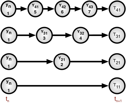
Figure 1: Structure of an Euler extrapolation step using the harmonic sequence ${1,2,3,4}$. Each numbered circle represents a function evaluation, and the numbers indicate the order in which they are performed.

2.1.2 Midpoint extrapolation (Ex-Midpoint)

It is common to perform extrapolation based on an integration method whose error function contains only even terms, such as the midpoint method [16, 34]. In this case, each extrapolation step raises the order of accuracy by two. We refer to this approach as Ex-Midpoint and give the algorithm below. Using midpoint extrapolation to obtain order $p$ requires about half as many stages, compared to Ex-Euler:

$$s =\frac{p^{2}+4}{4}.$$ (7)

Again, the number of stages grows quadratically with the order.

Algorithm 2 Explicit Midpoint extrapolation (Ex-Midpoint)

$r=p/2$

for $k=1\to r$ do $\triangleright$ Compute second-order approximations

     $Y_{k0}=y_{n}$

     $Y_{k1}=Y_{k,0}+\frac{h}{2k}f(Y_{k,0})$ $\triangleright$ Initial Euler step

     for $j=2\to 2k$ do

         $Y_{kj}=Y_{k,j-2}+\frac{h}{k}f(Y_{k,j-1})$ $\triangleright$ Midpoint steps

     end for

     $T_{k1}=Y_{k,2k}$

end for

for $k=2\to r$ do $\triangleright$ Extrapolate to get higher order

     for $j=k\to r$ do

         $T_{jk}=T_{j,k-1}+\frac{T_{j,k-1}-T_{j-1,k-1}}{\frac{j^{2}}{(j-k+1)^{2}}-1}$ $\triangleright$ Aitken-Neville formula for extrapolation to order 2k

     end for

end for

$y_{n+1}=T_{rr}$ $\triangleright$ New solution value

$\hat{y}_{n+1}=T_{r-1,r-1}$ $\triangleright$ Embedded method solution value

2.2 Deferred correction (DC-Euler)

Like extrapolation, deferred correction has a long history; its application to initial value problems goes back to [7]. Recently it has been revived as an area of research, see [10, 15] and subsequent works. Here we focus on the class of methods introduced in [10], with a modification introduced in [26]. These spectral DC methods are one-step methods and can be constructed for any order of accuracy.

Spectral DC methods start like extrapolation methods, by using a low-order method to step over subintervals of the time step; the subintervals can be equally sized, or Chebyshev nodes can be used. We consider methods based on the explicit Euler method and Chebyshev nodes. Subsequently, high-order polynomial interpolation of the computed values is used to approximate the integral of the error, or defect. Then the method steps over the same nodes again, applying a correction. This procedure is repeated until the desired accuracy is achieved.

A modification of the spectral DC method appears in [26], in which a parameter $\theta$ is used to adjust the dependence of the correction steps on previous iterations. The original scheme corresponds to $\theta=1$; by taking $\theta\in[0,1]$ the stability of the method can be improved. Given a fixed order of accuracy and a predictor method, the resulting spectral DC method can be written as a Runge–Kutta method [13]. The algorithm is defined below (the values $c_{j}$ denote the locations of the Chebyshev nodes) and depicted in Figure 2. For error estimation, we use the solution from the next-to-last correction iteration, whose order is one less than that of the overall method.

Algorithm 3 Explicit Euler-based deferred correction (DC-Euler)

$Y_{10}=y_{n}$

for $k=1\to p-1$ do $\triangleright$ Compute initial prediction

     $Y_{1k}=Y_{1,k-1}+(c_{k+1}-c_{k})hf(Y_{1,k-1})$

end for

for $k=2\to p$ do $\triangleright$ Compute successive corrections

     $Y_{k0}=y_{n}$

     for $j=1\to p-1$ do

         $Y_{kj}=Y_{k,j-1}+h\theta(f(Y_{k,j-1})-f(Y_{k-1,j-1}))+\mathcal{I}_{j-1}^{j}(f(Y_{k-1,:}))$

     end for

end for

$y_{n+1}=Y_{p,p-1}$ $\triangleright$ New solution value

$\hat{y}_{n+1}=Y_{p-1,p-1}$ $\triangleright$ New solution value

In Algorithm 3, $\mathcal{I}_{j-1}^{j}(f(Y_{k-1,:}))$ represents the integral of the degree $p-1$ polynomial that interpolates the points $Y_{k-1,j}$ for $j=1,\dots,p-1$, over the interval $[t_{n}+c_{j}h,t_{n}+c_{j+1}h]$. Thus, for $\theta=0$, the algorithm becomes a discrete version of Picard iteration.

The number of stages per step is

$$s=p(p-1)$$ (8)

unless $\theta=0$, in which case the stages $Y_{p,j}$ (for $j<p-1$) need not be computed at all since $Y_{p,p-1}$ depends only on the $Y_{p-1,j}$. Then the number of stages per step reduces to $(p-1)^{2}+1$.

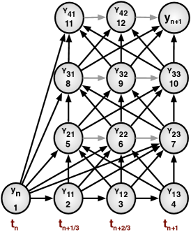
Figure 2: Structure of a 4th-order spectral DC step using 3 Euler substeps. Each numbered circle represents a function evaluation, and the numbers indicate the order in which they are performed. The black arrows represent dependencies; the grey arrows are dependencies that vanish when $\theta=0$. Note that node 1 is connected to all other nodes; some of those arrows have been omitted for clarity. Thus the solution at each node depends on all solutions from the previous iteration and, unless $\theta=0$, on its predecessor in the current iteration.

2.3 Reference Runge–Kutta methods

In this work we use the following existing Runge-Kutta pairs as benchmarks for evaluating extrapolation and deferred correction methods:

• Fourth order: the embedded formula of Merson 4(3) [16, pg. 167]

• Sixth order: the 6(5) pair of Calvo et. al. [4], which was found to be the most efficient out of those considered by Hosea and Shampine [17]

• Eighth order: the well-known Prince-Dormand 8(7) pair [30]

• Tenth order: the 10(8) pair of Curtis [6]

• Twelfth order: The 12(9) pair of Ono [29]

It should be stressed that finding pairs of order higher than eight is still very challenging, and the tenth- and twelfth-order pairs here are not expected to be as efficient as that of Prince-Dormand.

3 Concurrency

[P. Deuflhard, 1985] In view of an implementation on parallel computers, extrapolation methods (as opposed to RKp methods or multistep methods) have an important distinguishing feature: the rows can be computed independently.

If a Runge-Kutta method includes stages that are mutually independent, then those stages may be computed concurrently [20]. In this section we investigate theoretically achievable parallel speedup and efficiency of extrapolation and deferred correction methods. Our goal is to determine hardware- and problem- independent upper bounds based purely on algorithmic concerns. We do not attempt to account for machine-specific overhead or communication, although the simple parallel tests in Section 5.5 suggest that the bounds we give are realistically achievable for at least some classes of moderate-sized problems. Previous works that have considered concurrency in explicit extrapolation and deferred correction methods include [33, 34, 31, 2, 14, 11, 21, 27, 28].

3.1 Computational model and speedup

As in the serial case, our computational model is based on the assumption that evaluation of $f$ is sufficiently expensive so that all other operations (e.g., arithmetic, step size selection) are negligible by comparison.

Typically, stage $y_{j}$ of an explicit Runge–Kutta method depends on all the previous stages $y_{1},y_{2},\dots,y_{j-1}$. However, if $y_{j}$ does not depend on $y_{j-1}$, then these two stages may be computed simultaneously on a parallel computer. More generally, by interpreting the incidence matrix of $A$ as the adjacency matrix of a directed graph $G(A)$, one can determine precisely which stages may be computed concurrently and how much speedup may be achieved. For extrapolation methods, the computation of each $T_{k1}$ may be performed independently in parallel [9], as depicted in Figure 3. Unlike some previous authors, we do not consider parallel implementation of the extrapolation process (i.e., the second loop in Algorithm 1) since it does not include any evaluations of $f$ (so our computational model assumes its cost is negligible anyway).

For the deferred correction methods we consider, parallel computation is advantageous only if $\theta=0$; the resulting parallel algorithm is depicted in Figure 4. A different approach to parallelism in DC methods is taken by the RIDC method [5]; see also [14]. Deferred correction has also been combined with the parareal algorithm to achieve parallel speedup [28, 11].

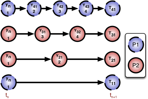
Figure 3: Exploiting concurrency in an Euler extrapolation step using 2 processes. The blue circles with broken border are computed by process 1 and the red circles with solid border are computed by process 2. Observe that only $s_{\textup{seq}}=4$ sequential function evaluations are required for each process, as opposed to the $s=7$ sequential evaluations required in serial.

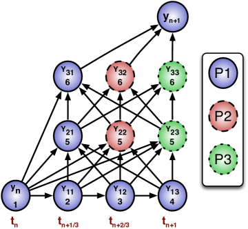
Figure 4: Exploiting concurrency in a 4th-order spectral DC step (with $\theta=0$) using 3 Euler substeps and 3 processes. The color and border of each circle indicate which process evaluates it. Observe that only $s_{\textup{seq}}=6$ sequential function evaluations are required for each process, as opposed to the $s=10$ sequential evaluations required in serial (12 in serial when $\theta\neq 0$). Note that node 1 is connected to all other nodes; some of those arrows have been omitted for clarity. More synchronization is required than for a similar extrapolation step.

We define the minimum number of sequential stages $s_{\textup{seq}}$ as the minimum number of sequential function evaluations that must be made when parallelism is taken into account. To make this more precise, let us label each node in the graph $G(A)$ by the index of the stage it corresponds to, with the node corresponding to $y_{n+1}$ labeled $s+1$. Then

$$s_{\textup{seq}}=\max_{j}\{\text{ path length from node $1$ to node $s+1$}\}.$$ (9)

The quantity $s_{\textup{seq}}$ represents the minimum time required to take one step with a given method on a parallel computer, in units of the cost of a single derivative evaluation. For instance, the maximum path length for the method shown in Figure 3 is equal to 4; for the method in Figure 4 it is 6. The maximum potential parallel speedup is

$$S =s/s_{\textup{seq}}.$$ (10)

The minimum number of processes required to achieve speedup $S$ is denoted by $P$ (equivalently, $P$ is the maximum number of processes that can usefully be employed by the method). Finally, let $E$ denote the theoretical parallel efficiency (here we use the term in the sense that is common in the parallel computing literature) that could be achieved by spreading the computation over $P$ processes:

$$E=\frac{s}{Ps_{\textup{seq}}}=\frac{S}{P}.$$ (11)

Note that $E$ is an upper bound on the achievable parallel efficiency; it accounts only for inefficiencies due to load imbalancing. It does not, of course, account for additional implementation-dependent losses in efficiency due to overhead or communication.

Table 1 shows the parallel algorithmic properties of fixed-order extrapolation and deferred correction methods. Note that for deferred correction methods with $\theta\neq 0$, we have $s_{\textup{seq}}=s$, i.e., no parallel computation of stages is possible.

Method	$s$	$s_{\textup{seq}}$	$S$	$P$	$E$
Ex-Euler	$\frac{p^{2}-p+2}{2}$	$p$	$\frac{p^{2}-p+2}{2p}$	$\lceil\frac{p}{2}\rceil$	$\frac{p^{2}-p+2}{2p\lceil\frac{p}{2}\rceil}$
Ex-Midpoint	$\frac{p^{2}+4}{4}$	$p$	$\frac{p^{2}+4}{4p}$	$\lceil\frac{p+2}{4}\rceil$	$\frac{p^{2}+4}{4p\lceil\frac{p+2}{4}\rceil}$
DC-Euler, $\theta=0$	$(p-1)^{2}+1$	$2(p-1)$	$\frac{(p-1)^{2}+1}{2(p-1)}$	$p-1$	$\frac{(p-1)^{2}+1}{2(p-1)}$
DC-Euler, $\theta\neq 0$	$p(p-1)$	$p(p-1)$	1	1	-

Table 1: Parallel implementation properties of extrapolation and deferred correction methods. $s$: number of stages; $s_{\textup{seq}}$: number of sequentially dependent stages; $S=s/s_{\textup{seq}}$: optimal speedup; $P$: number of processes required to achieve optimal speedup; $E=S/P$: parallel efficiency.

To our knowledge, no parallel implementation has been made of the deferred correction methods we consider here. However, the parallel iterated RK methods of [35] have a similar flavor. For parallel implementation of a revisionist DC method, see [5].

4 Theoretical measures of efficiency

Here we describe the theoretical metrics we use to evaluate the methods. Our metrics are fairly standard; a useful and thorough reference is [22]. The overarching metric for comparing methods is efficiency: the number of function evaluations required to integrate a given problem over a specified time interval to a specified accuracy. We assume that function evaluations are relatively expensive so that other arithmetic operations and overhead for things like step size selection are not significant.

The number of function evaluations is the product of the number of stages of the method and the number of steps that must be taken. The number of steps to be taken depends on the step size $h$, which is usually determined adaptively to satisfy accuracy and stability constraints, i.e.

$$h=\min(h_{\textup{stab}},h_{\textup{acc}})$$ (12)

where $h_{\textup{stab}},h_{\textup{acc}}$ are the maximum step sizes that ensure numerical stability and prescribed accuracy, respectively. Since the cost of a step is proportional to the number of stages of the method, $s$, then a fair measure of efficiency is $h/s$. A simple observation that partially explains results in this section is as follows: extrapolation and deferred correction are straightforward approaches to creating methods that satisfy the huge numbers of order conditions for very high order Runge–Kutta methods. However, this straightforward approach comes with a cost: they use many more than the minimum necessary number of stages to achieve a particular order, leading to relatively low efficiency.

4.1 Absolute stability

The stable step size $h_{\textup{stab}}$ is typically the limiting factor when a very loose error tolerance is applied. A method’s region of absolute stability (in conjunction with the spectrum of $f^{\prime}$) typically dictates $h_{\textup{stab}}$.

In order to make broad comparisons, we measure the size of the and real-axis interval that is contained in the absolute stability region. Specifically, let $S\subset\mathbb{C}$ denote the region of absolute stability; then we measure

$$I_{\textup{real}} =\max\{r\geq 0:[-r,0]\subset S\}$$ (13)

$$I_{\textup{imag}} =\max\{r\geq 0:[-ir,ir]\subset S\}.$$ (14)

Determination of the stability region for very high order methods can be numerically delicate; for instance, the stability function for the 8th-order deferred correction method is a polynomial of degree 56! Because of this, all stability calculations presented here have been performed using exact (rational) arithmetic, not in floating point.

Figure 5(a) and Table 2 show real and imaginary stability interval sizes for Ex-Euler, Ex-Midpoint, and DC-Euler methods of orders 4-12. We show the real stability intervals of the deferred correction methods with three different values of $\theta$, because this interval has a strong dependence on $\theta$. For all classes of methods, the overall size of the stability region grows with increasing order. However, many methods have $I_{\textup{imag}}=0$. Note that the stability regions for Ex-Euler and Ex-Midpoint are identical since both have stability polynomial

$$\sum_{k=0}^{p}\frac{z^{p}}{p!},$$ (15)

i.e., the degree-$p$ Taylor polynomial of the exponential function.

A fair metric for efficiency is obtained by dividing these interval sizes by the number of stages in the method. The result is shown in Figure 5(b). Higher-order methods have smaller relative stability regions. For orders $p\leq 10$, the reference RK methods have better real stability properties. We caution that, for high order methods, the boundary of the stability region typically lies very close to the imaginary axis, so values of the amplification factor may differ from unity by less than roundoff over a large interval. For instance, the 10th-order extrapolation method has $I_{\textup{imag}}=0$, but the magnitude of its stability polynomial differs from unity by less than $1.4\times 10^{-15}$ over the interval $[-i/4,i/4]$. It is not clear whether precise measures of $I_{\textup{imag}}$ are relevant for such methods in practical situations.

Here for simplicity we have considered only the stability region of the principal method; in the design of embedded pairs, it is important that the embedded method have a similar stability region. All the pairs considered here seem to have fairly well matched stability regions.

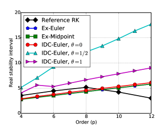
(a) Real Stability Interval

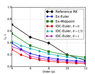
(b) Scaled Real Stability Interval

Figure 5: Comparison of stability regions for reference methods, Euler extrapolation, midpoint extrapolation and deferred correction.

Order	Reference RK	Ex-Euler	Ex-Midpoint	DC-Euler, $\theta=0$
4	3.46	2.83	2.83	2.93
5	-	0	-	0
6	2.61	0	0	0
7	-	1.76	-	1.82
8	0	3.40	3.40	3.52
9	-	0	-	0
10	0	0	0	0
11	-	1.70	-	1.75

Table 2: Imaginary stability intervals.

4.2 Accuracy efficiency

Typically, the local error is controlled by requiring that $\|y_{n+1}-\hat{y}_{n+1}\|<\epsilon$ for some tolerance $\epsilon>0$. When the maximum stable step size does not yield sufficient accuracy, the accuracy constraint determines the step size. This is typically the case when the error tolerance is reasonably small. In theoretical analyses, the principal error norm [22]

$$C_{p+1} =\left(\sum_{k}(\tau_{k}^{(p+1)})^{2}\right)^{\frac{1}{2}}$$ (16)

is often used as a way to compare accuracy between two methods of the same order. Here the constants $\tau_{k}^{(p+1)}$ are the coefficients appearing in the leading order truncation error terms.

Assuming that the one-step error is proportional to $C_{p+1}h^{p+1}$ leads to a fair comparison of accuracy efficiency given by the accuracy efficiency index, introduced in [17]:

$$\eta=\frac{1}{s}\left(\frac{1}{C_{p+1}}\right)^{1/p+1}.$$ (17)

Figure 6(a) plots the accuracy efficiency index for the methods under consideration. Interestingly, a ranking of methods based on this metric gives the same ordering as that based on $I_{\textup{real}}/s$.

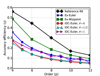
(a) Serial accuracy efficiency

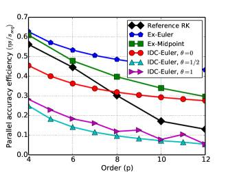
(b) Ideal parallel accuracy efficiency

Figure 6: Accuracy efficiency

4.3 Accuracy and stability metrics

In order to determine idealized accuracy and stability efficiency measures, we take the speedup factor $s/s_{\textup{seq}}$ into account. In other words, we consider

$$\frac{s}{s_{\textup{seq}}}\eta=\frac{1}{s_{\textup{seq}}}\left(\frac{1}{C_{p+1}}\right)^{1/p+1},$$ (18)

as a measure of accuracy efficiency. A similar scaling could be used to study stability efficiency of parallel implementations. We stress that in this context efficiency relates to the number of function evaluations required to advance to a given time, and is not related to the usual concept of parallel efficiency.

Figure 6(b) shows the accuracy efficiency, rescaled by the speedup factor. Comparing with Figure 6(a), we see a very different picture for methods of order 8 and above. Extrapolation methods are the most efficient, while the reference RK methods give the weakest showing – since they do not benefit from parallelism.

4.4 Predictions

The theoretical measures above indicate that fixed-order extrapolation and deferred correction methods are less efficient than traditional Runge–Kutta methods, at least up to order eight. At higher orders, the disadvantage of extrapolation and spectral DC are less pronounced, but they still offer no theoretical advantage. When parallelism is taken into account, extrapolation and deferred correction offer a significant theoretical advantage.

5 Performance tests

In this section we perform numerical tests, solving some initial value problems with the methods under consideration, to validate the theoretical predictions of the last section.

In addition to the tests shown, we tested all methods on a collection of problems known as the non-stiff DETEST suite [18]. The results (not shown here) are broadly consistent with those seen in the test problems below.

5.1 Verification tests

For each of the pairs considered, we performed convergence tests using a sequence of fixed step sizes with several nonlinear systems of ODEs, in order to verify that the expected rate of convergence is achieved in practice. We also checked that the coefficients of each method satisfy the order conditions exactly (in rational arithmetic).

5.2 Step size control

For step size selection, we use a standard $I$-controller [22]:

$$h_{n+1}^{*}=\kappa h_{n}\left(\frac{\epsilon}{||\delta_{n+1}||_{\infty}}\right)^{\alpha}.$$ (19)

Here $\epsilon$ is the chosen integration tolerance and $\delta_{n+1}=y_{n+1}-\hat{y}_{n+1}$. We take $\kappa=0.9$ and $\alpha=0.7/p$, where $p$ is the order of the embedded method. The step size is not allowed to increase or decrease too suddenly; we use [16]:

$$h_{n+1}=\text{min}\left(\kappa_{max}h_{n},\text{max}\left(\kappa_{min}h_{n},h^{*}_{n+1}\right)\right)$$ (20)

with $\kappa_{min}=0.2$ and $\kappa_{max}=5$. A step is rejected if the error estimate exceeds the tolerance; i.e., if $\|\delta_{n}\|_{\infty}>\epsilon$.

All tests in this work were also run with a $PI$-controller, and very similar results were obtained.

5.3 Test problems and results

5.3.1 Three-body problem

We consider the first three-body problem from [32]:

$$\text{SB1}:\qquad\qquad y_{1}^{\prime} =y_{3},$$ (21)

$$y_{2}^{\prime} =y_{4},$$

$$y_{3}^{\prime} =y_{1}+2y_{4}-\mu^{\prime}\frac{y_{1}+\mu}{\left((y_{1}+\mu)^{2}+y_{2}^{2}\right)^{\frac{3}{2}}}-\mu\frac{y_{1}-\mu^{\prime}}{\left((y_{1}-\mu^{\prime})^{2}+y_{2}^{2}\right)^{\frac{3}{2}}}$$

$$y_{4}^{\prime} =y_{2}+2y_{3}-\mu^{\prime}\frac{y_{2}}{\left((y_{1}+\mu)^{2}+y_{2}^{2}\right)^{\frac{3}{2}}}-\mu\frac{y_{2}}{\left((y_{1}-\mu^{\prime})^{2}+y_{2}^{2}\right)^{\frac{3}{2}}},$$

Here $\mu^{\prime}=1-\mu$, the final time is $T=6.192169331319639$, and the initial values are

$$y_{1}(0)=1.2,\;y_{2}(0)=0,\;y_{3}(0)=0,\;y_{4}(0)=-1.049357509830319\text{ and }\mu=0.0121285627653123.$$ (22)

Figure 7 plots number of function evaluations (cost) against the absolute error for this problem. The absolute error is

$$\textup{Error}=|y_{N}-y(T)|,$$ (23)

where $T$ is the final time and $y_{N}$ is the numerical solution at that time, while $y(T)$ is a reference solution computed using a fine grid and the method of Bogacki & Shampine [1]. The initial step size is 0.01. In every case, the method efficiencies follow the ordering predicted by the accuracy efficiency index, and are consistent with previous studies.

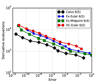
(a) 6th order

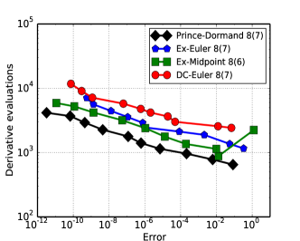
(b) 8th order

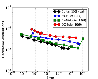
(c) 10th order

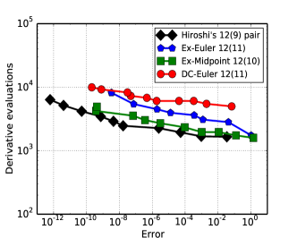
(d) 12th order

Figure 7: Efficiency tests on problem SB1 (Section 5.3.1).

5.3.2 A two-population growth model

Next we consider problem B1 of [18], which models the growth of two conflicting populations:

$$y_{1}^{\prime} =2(y_{1}-y_{1}y_{2}) y_{1}(0) =1$$ (24a)

$$y_{2}^{\prime} =-(y_{2}-y_{1}y_{2}) y_{2}(0) 3.$$ (24b)

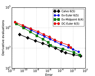
(a) 6th order

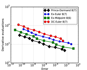
(b) 8th order

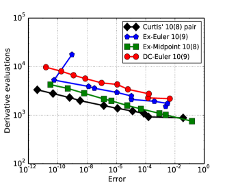
(c) 10th order

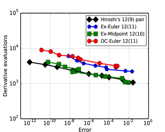
(d) 12th order

Figure 8: Efficiency tests on problem B1 (Section 5.3.2).

5.3.3 A nonlinear wave PDE

Finally, we consider the integration of a high-order PDE semi-discretization from [23]. We solve the 1D elasticity equations

$$\epsilon_{t}(x,t)-u_{x}(x,t) =0$$ (25a)

$$\rho(x)u(x,t)_{t}-\sigma(\epsilon(x,t),x)_{x} =0.$$ (25b)

with nonlinear stress-strain relation

$$\sigma(\epsilon,x)=\exp(K(x)\epsilon)-1,$$ (26)

and a simple periodic medium composed of alternating homogeneous layers:

$$\rho(x)=K(x) =\left\{\begin{array}[]{ll}4&\text{if }j<x<(j+1/2)\mbox{ for some integer j},\\ 1&\mbox{otherwise.}\end{array}\right.$$ (29)

We consider the domain $0\leq x\leq 300$, an initial Gaussian perturbation to the stress, and final time $T=100$. The solution consists of two trains of emerging solitary waves; one of them is depicted in Figure 9(a). The semi-discretization is based on the WENO wave-propagation method implemented in SharpClaw [25].

Efficiency results for 8th order methods are shown in Figure 9(b). The spatial grid is held fixed across all runs, and the time step is adjusted automatically to satisfy the imposed tolerance. The error is computed with respect to a solution computed with tolerance $10^{-13}$ using the 5(4) pair of Bogacki and Shampine. For the most part, these are consistent with the results from the smaller problems above. However, the midpoint extrapolation method performs quite poorly on this problem. The reason is not clear, but this underscores the fact that performance on particular problems can be very different from the “average” performance of a method.

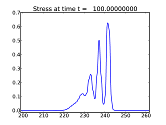
(a) Solution (stress)

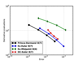
(b) Efficiency

Figure 9: Solution and efficiency for methods applied to the stegoton problem (Section 5.3.3).

5.4 Failure of integrators

Some failure of the integrators was observed in testing. These failures fall into two categories. First, at very tight tolerances, the high order Euler extrapolation methods were sometimes unable to finish because the time step size was driven to zero. This is a known issue related to internal stability; for a full explanation see [24].

Second, the deferred correction methods sometimes gave global errors much larger than those obtained with the other methods. This indicates a failure of the error estimator. Upon further investigation, we found that the natural embedded error estimator method of order $p-1$ satisfies nearly all (typically all but one) of the order conditions for order $p$. Hence these estimators may be said to be defective, and it would be advisable to employ a more robust approach like that discussed in [10]. Since our focus is purely on Runge–Kutta pairs, we do not pursue this issue further here.

5.5 Ideal parallel performance

Figures 10-12 show efficiency for the same three test problems but now based on the number of sequential evaluations. That is, the vertical axis is $Ns_{\textup{seq}}$, where $N$ denotes the number of steps taken. The same measure of efficiency was used in [35]. We see that the parallelizable methods – especially extrapolation – outperform traditional methods, especially at higher orders. Similar results were obtained for parallel iterated RK methods in [35]. Remarkably, the deferred correction method performs the best by this measure for the stegoton problem.

This measure of efficiency may be viewed with some skepticism since it neglects the cost of communication. This concern is addressed with a true parallel implementation in the next section.

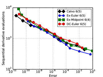
(a) 6th order methods

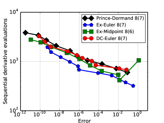
(b) 8th order methods

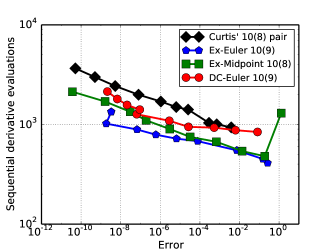
(c) 10th order methods

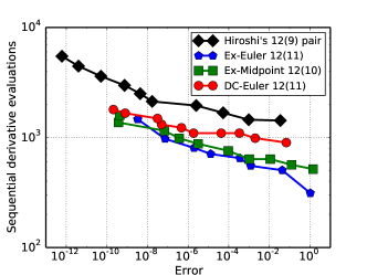
(d) 12th order methods

Figure 10: Efficiency for the problem SB1 (Section 5.3.1) based on sequential derivative evaluations.

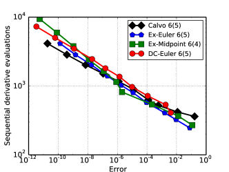
(a) 6th order methods

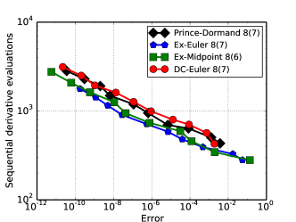
(b) 8th order methods

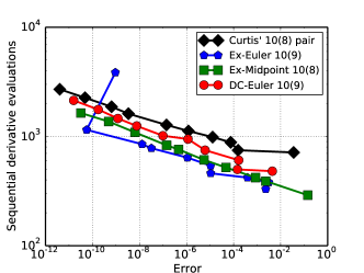
(c) 10th order methods

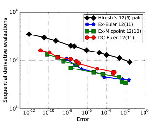
(d) 12th order methods

Figure 11: Efficiency for the problem B1 (Section 5.3.2) based on sequential derivative evaluations.

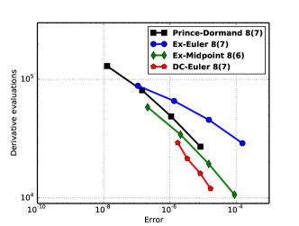
Figure 12: Parallel efficiency for the stegoton problem (Section 5.3.3).

6 A shared-memory implementation of extrapolation

Development and testing of a tuned parallel extrapolation or deferred correction code is beyond the scope of this paper, but in this section we run a simple example to demonstrate that it is possible in practice to achieve speedups like those listed in Table 1, and to outperform even the best highly-tuned traditional RK methods, at least on problems with an expensive right-hand-side. We focus on speedup with an eye to providing efficient black-box parallel ODE integrators for multicore machines, noting that the number of available cores is often more than can be advantageously used by the methods considered.

Previous studies have implemented explicit extrapolation methods in parallel and achieved parallel efficiencies of up to about 80% [19, 21, 27]. As those studies were conducted about twenty years ago, it is not clear that their conclusions are relevant to current hardware.

In order to test the achievable parallel speedup, we took the code ODEX [16], downloaded from http://www.unige.ch/~hairer/software.html, and modified it as follows:

• Fixed the order of accuracy (disabling adaptive order selection)

• Inserted an OMP PARALLEL pragma around the extrapolation loop

• Removed the smoothing step

We refer to the modified code as ODEX-P.

Figure 13(a) shows the achieved speedup based on dynamic scheduling for $p=6,10,14,18$, applying the code to an $N$-body gravitational problem with 400 bodies. Results for other orders are similar. The dotted lines show the theoretical maximum speedup $S=(p^{2}+4)/(4p)$ based on our earlier analysis. The tests were run on a workstation with two 2.66 Ghz quad-core Intel Xeon processors, and the code was compiled using gfortran. Using $p/2$ threads, the measured speedup is very close to the theoretical maximum. However, the speedup is significantly below the theoretical value when only $P$ threads are used. We interpret this to mean that the dynamic scheduler is not able to optimally allocate the work among threads unless there are enough threads to give just one loop iteration to each.

Figure 13(b) and Table 3 show the result of a more intelligent parallel implementation, using static scheduling with the code modified so that both $T_{k1}$ and $T_{r-k,1}$ are computed in a single loop iteration. This load balancing scheme is optimal when using on the optimal number of threads $P$, and the results agree almost perfectly with theory.

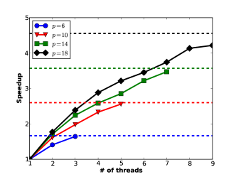
(a) Dynamic scheduling

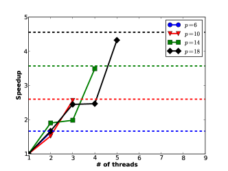
(b) Manual load-balancing

Figure 13: Measured speedup of the midpoint extrapolation code ODEX-P on a 400-body gravitation problem by insertion of a single OMP parallel pragma in the code. The ratio of runtime with multiple threads to runtime using a single thread is plotted. The dotted lines show the theoretical maximum speedup $S=(p^{2}+4)/(4p)$ based on our earlier analysis.

		Runtime		Max. speedup		Parallel Efficiency
Order ($p$)	$P$	1 thread	$P$ threads	Theory ($S$)	Observed	Theory ($E$)	Observed
6	2	13.140	7.977	1.67	1.65	0.83	0.82
10	3	17.370	6.770	2.60	2.57	0.87	0.86
14	4	19.508	5.573	3.57	3.50	0.89	0.88
18	5	25.876	5.827	4.56	4.44	0.91	0.89

Table 3: Runtime, speedup and efficiency of manually load-balanced runs of the modified ODEX-P code with $P$ threads. The observed speedup (and efficiency) are close to the theoretically optimal values ($S$ and $E$).

6.1 Comparison with DOP853

We now compare actual runtimes of our experimental ODEX-P with the DOP853 code available from http://www.unige.ch/~hairer/prog/nonstiff/dop853.f. These two codes have been compared in [16, Section II.10], but using the original ODEX code (with order-adaptivity and without parallelism). In that reference, DOP853 was shown to be superior to ODEX at all but the most strict tolerances.

Table 4 shows runtimes versus prescribed tolerance for a 400-body problem for the two codes, using fixed order 12 (with 4 threads) in the ODEX-P code. Figure 14 shows the achieved relative root-mean-square global error versus runtime. Perhaps surprisingly, the parallel extrapolation code is no worse even at loose tolerances. At moderate to strict tolerances, it substantially outperforms the RK code.

	Tolerance
Code	1.e-3	1.e-5	1.e-7	1.e-9	1.e-11
DOP853	3.81	9.02	17.80	30.93	56.75
ODEX-P(12)	3.31	5.87	10.32	18.07	26.76

Table 4: Runtimes (in seconds) for Dormand-Prince and modified 12th-order ODEX-P code. The tests were run on a workstation with two 2.66 Ghz quad-core Intel Xeon processors using four threads.

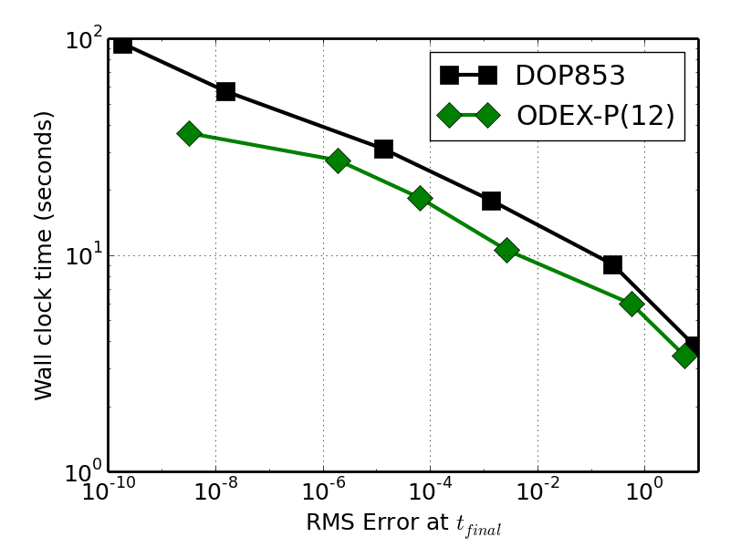
Figure 14: Runtime versus achieved relative error of the midpoint extrapolation code ODEX-P on a 400-body gravitation problem. The tests were run on a workstation with two 2.66 Ghz quad-core Intel Xeon processors using four threads.

7 Discussion

This study is intended to provide a broadly useful characterization of the properties of explicit extrapolation and spectral deferred correction methods. Of course, no study like this can be exhaustive. Our approach handicaps extrapolation and deferred correction methods by fixing the order throughout each computation; practical implementations are order-adaptive and should achieve somewhat better efficiency. We have investigated only the most generic versions of each class of methods; other approaches (e.g., using higher order building blocks or exploiting concurrency in different ways) may give significantly different results. Such approaches could be evaluated using the same kind of analysis employed here. Finally, our parallel computational model is valid only when evaluation of $f$ is relatively expensive – but that is when efficiency and concurrency are of most interest.

The most interesting new conclusions from the present study is that parallel extrapolation methods of very high order outperform sophisticated implementations of the best available RK methods for problems with an expensive right hand side. This is true even for a relatively naive non-order-adaptive code. We have shown that near-optimal speedup can be achieved in practice with simple modification of an existing code. The resulting algorithm is faster (at least for some problems) than the highly-regarded DOP853 code.

Our serial results are in line with those of previous studies. New here is the evidence that spectral deferred correction – like extrapolation – seems inferior to well-designed RK methods (in serial). However, we have tested only one of the many possible variants of these methods.

High order Euler extrapolation methods suffer from dramatic amplification of roundoff errors. This leads to the loss of several digits of accuracy (and failure of the automatic error control) for very high order methods, and is observed in practice on most problems. Fortunately, midpoint extrapolation does not exhibit this amplification.

The theoretical and preliminary experimental results we have presented suggest that a carefully-designed parallel code based on midpoint extrapolation could be very efficient. Such a practical implementation is the subject of current efforts.

Acknowledgment. We thank one of the referees, who pointed out a discrepancy that revealed an important bug in our implementation of some spectral deferred correction methods when $\theta\neq 0$.

References

- [1] P Bogacki and Lawrence F Shampine. An efficient Runge-Kutta (4, 5) pair. Computers & Mathematics with Applications, 32(6):15–28, 1996.
- [2] Kevin Burrage. Parallel and sequential methods for ordinary differential equations. Clarendon Press, 1995.
- [3] J. C. Butcher. Numerical Methods for Ordinary Differential Equations. Wiley, 2nd edition, 2008.
- [4] M. Calvo, J.I. Montijano, and L. Randez. A new embedded pair of Runge-Kutta formulas of orders 5 and 6. Computers & Mathematics with Applications, 20(1):15–24, 1990.
- [5] Andrew J. Christlieb, Colin B. Macdonald, and Benjamin W. Ong. Parallel high-order integrators. SIAM Journal on Scientific Computing, 32(2):818–835, Jan 2010.
- [6] A. R. Curtis. High-order explicit Runge-Kutta formulae, their uses, and limitations. IMA Journal of Applied Mathematics, 16(1):35–52, 1975.
- [7] James W. Daniel, Victor Pereyra, and Larry L. Schumaker. Iterated deferred corrections for initial value problems. Acta Cientifica Venezolana, 19:128–135, 1968.
- [8] P. Deuflhard. Order and stepsize control in extrapolation methods. Numerische Mathematik, 41(3):399–422, 1983.
- [9] P. Deuflhard. Recent progress in extrapolation methods for ordinary differential equations. SIAM Review, 27(4):505–535, December 1985.
- [10] A. Dutt, L. Greengard, and Vladimir Rokhlin. Spectral deferred correction methods for ordinary differential equations. BIT Numerical Mathematics, 40:241–266, 2000.
- [11] Matthew Emmett and Michael Minion. Toward an efficient parallel in time method for partial differential equations. Comm. App. Math. and Comp. Sci, 7(1):105–132, 2012.
- [12] T Feagin. High-order explicit Runge-Kutta methods using M-symmetry. Neural Parallel and Scientific Computations, 20(3):437, 2012.
- [13] Sigal Gottlieb, David I. Ketcheson, and Chi-Wang Shu. High order strong stability preserving time discretizations. Journal of Scientific Computing, 38(3):251–289, 2009.
- [14] D Guibert and D Tromeur-Dervout. Cyclic distribution of pipelined parallel deferred correction method for ODE/DAE. In Parallel Computational Fluid Dynamics 2007, pages 171–178. Springer, 2009.
- [15] Bertil Gustafsson and Wendy Kress. Deferred correction methods for initial value problems. BIT Numerical Mathematics, 41(5):986–995, 2001.
- [16] Ernst Hairer, Syvert P. Nø rsett, and G. Wanner. Solving ordinary differential equations I: Nonstiff Problems. Springer Series in Computational Mathematics. Springer, Berlin, second edition, 1993.
- [17] M.E. Hosea and L.F. Shampine. Efficiency comparisons of methods for integrating ODEs. Computers & Mathematics with Applications, 28(6):45–55, September 1994.
- [18] T. E. Hull, W. H. Enright, B. M. Fellen, and A. E. Sedgwick. Comparing Numerical Methods for Ordinary Differential Equations. SIAM Journal on Numerical Analysis, 9(4):603–637, December 1972.
- [19] Takashi Ito and Toshio Fukushima. Parallelized extrapolation method and its application to the orbital dynamics. The Astronomical Journal, 114:1260, Sep 1997.
- [20] K. R. Jackson and S. P. Nørsett. The potential for parallelism in Runge-Kutta methods . part 1 : Rk formulas in standard form. 32(1):49–82, 2012.
- [21] M. Kappeller, M. Kiehl, M. Perzl, and M. Lenke. Optimized extrapolation methods for parallel solution of IVPs on different computer architectures. Applied Mathematics and Computation, 77(2-3):301–315, Jul 1996.
- [22] C. A. Kennedy, M. H. Carpenter, and R Michael Lewis. Low-storage, explicit Runge–-Kutta schemes for the compressible Navier–-Stokes equations. Applied Numerical Mathematics, 35(3):177–219, November 2000.
- [23] David I. Ketcheson and Randall J. LeVeque. Shock dynamics in layered periodic media. Communications in Mathematical Sciences, 10(3):859–874, 2012.
- [24] David I Ketcheson, Lajos Lóczi, and Matteo Parsani. Internal error propagation in explicit Runge–Kutta discretization of PDEs. Preprint available from http://arxiv.org/abs/1309.1317, 2013.
- [25] DI Ketcheson, Matteo Parsani, and RJ LeVeque. High-order Wave Propagation Algorithms for Hyperbolic Systems. SIAM Journal on Scientific Computing, 35(1):A351–A377, 2013.
- [26] Y Liu, CW Shu, and M Zhang. Strong stability preserving property of the deferred correction time discretization. Journal of Computational Mathematics, 2007.
- [27] L Lustman, B Neta, and W Gragg. Solution of ordinary differential initial value problems on an intel hypercube. Computers & Mathematics with Applications, 23(10):65–72, 1992.
- [28] Michael Minion. A hybrid parareal spectral deferred corrections method. Communications in Applied Mathematics and Computational Science, 5:265–301, 2010.
- [29] Hiroshi Ono. On the 25 stage 12th order explicit Runge-Kutta method. Transactions-Japan Society for Industrial and Applied Mathematics, 16(3):177, 2006.
- [30] P.J. Prince and J.R. Dormand. High order embedded Runge-Kutta formulae. Journal of Computational and Applied Mathematics, 7(1):67–75, March 1981.
- [31] Thomas Rauber and Gudula Rünger. Load balancing schemes for extrapolation methods. Concurrency: Practice and Experience, 9(3):181–202, 1997.
- [32] L. F. Shampine and L. S. Baca. Fixed versus variable order Runge-Kutta. ACM Transactions on Mathematical Software, 12(1):1–23, May 1986.
- [33] HH Simonsen. Extrapolation methods for ODE’s: continuous approximations, a parallel approach. PhD thesis, PhD thesis, University of Trondheim, Norway, 1990.
- [34] P. J. van der Houwen and B. P. Sommeijer. Parallel ODE solvers. ACM SIGARCH Computer Architecture News, 18(3):71–81, September 1990.
- [35] Peter J Van Der Houwen and Benjamin P Sommeijer. Parallel iteration of high-order runge-kutta methods with stepsize control. Journal of Computational and Applied Mathematics, 29(1):111–127, 1990.