Pion form factor and reactions $e^{+}e^{-}\to\omega\pi^{0}$ and $e^{+}e^{-}\to\pi^{+}\pi^{-}\pi^{+}\pi^{-}$ at energies up to 2-3 GeV in the many-channel approach.

Abstract

Using the field-theory-inspired expression for the pion electromagnetic form factor $F_{\pi}$, a good description of the data in the range $-10<s<1$ GeV² is obtained upon taking into account the pseudoscalar-pseudoscalar (PP) loops. When the vector-pseudoscalar (VP) and the axial vector-pseudoscalar (AP) loops are taken into account in addition to the PP ones, a good description of the $BABAR$ data on the reaction $e^{+}e^{-}\to\pi^{+}\pi^{-}$ is obtained at energies up to 3 GeV. The inclusion of the VP and AP loops demands the treatment of the reactions $e^{+}e^{-}\to\omega\pi^{0}$ and $e^{+}e^{-}\to\pi^{+}\pi^{-}\pi^{+}\pi^{-}$. This task is performed with the SND data on $\omega\pi^{0}$ production and the $BABAR$ data on $\pi^{+}\pi^{-}\pi^{+}\pi^{-}$ production, both in $e^{+}e^{-}$ annihilation, by taking into account $\rho(770)$ and the heavier $\rho(1450)$, $\rho(1700)$, and $\rho(2100)$ resonances. The problems arising from including of the VP and AP loops are pointed out and discussed.

I Introduction

Some time ago we suggested a new expression for the electromagnetic form factor of the pion $F_{\pi}$ ach11 ; ach12 ; ach13 , which describes the data on the reaction $e^{+}e^{-}\to\pi^{+}\pi^{-}$ snd ; cmd ; kloe ; babar restricted to the time-like region $4m^{2}_{\pi}<s\leq 1$ GeV². The expression takes into account the strong resonance mixing via common decay modes and the $\rho\omega$ mixing. It has both the correct analytical properties and the normalization condition $F_{\pi}(0)=1$, and can be represented in the form:

$$F_{\pi}(s) = \frac{1}{\Delta}(g_{\gamma\rho_{1}},g_{\gamma\rho_{2}},g_{\gamma\rho_{3}},...)\left(\begin{array}[]{ccccc}g_{11}&g_{12}&g_{13}&...&\frac{g_{11}\Pi_{\rho_{1}\omega}}{D_{\omega}}\\ g_{12}&g_{22}&g_{23}&...&\frac{g_{12}\Pi_{\rho_{1}\omega}}{D_{\omega}}\\ g_{13}&g_{23}&g_{33}&...&\frac{g_{13}\Pi_{\rho_{1}\omega}}{D_{\omega}}\\ ...&...&...&...&...\\ \frac{g_{11}\Pi_{\rho_{1}\omega}}{D_{\omega}}&\frac{g_{12}\Pi_{\rho_{1}\omega}}{D_{\omega}}&\frac{g_{13}\Pi_{\rho_{1}\omega}}{D_{\omega}}&...&\frac{\Delta}{D_{\omega}}\\ \end{array}\right)\left(\begin{array}[]{c}g_{\rho_{1}\pi\pi}\\ g_{\rho_{2}\pi\pi}\\ g_{\rho_{3}\pi\pi}\\ ...\\ 0\\ \end{array}\right),$$ (11)

where $i$ ($i=1,2,3,...$) counts the $\rho$-like resonance states $\rho_{1}\equiv\rho(770)$, $\rho_{2}\equiv\rho(1450)$, $\rho_{3}\equiv\rho(1700)$, …, the quantity

$$g_{\gamma V}=\frac{m^{2}_{V}}{g_{V}},$$ (12)

($V=\rho_{1,2,3,...},\omega$) is introduced in such a way that $eg_{\gamma V}$ is the $\gamma V$ transition amplitude, where $e$ is the electric charge. As usual, the coupling constant $g_{V}$ is calculated from the electronic width

$$\Gamma_{V\to e^{+}e^{-}}=\frac{4\pi\alpha^{2}m_{V}}{3g^{2}_{V}}$$ (13)

of the resonance $V$. The quantities $g_{ij}/\Delta$ are the matrix elements of the matrix $G^{-1}$ given by Eq. (59) below, and $\Delta={\rm det}G$. Ellipses mean additional states like $\rho(2100)$ etc. It is assumed that the direct G-parity-violating decay $\omega\to\pi^{+}\pi^{-}$ is absent, that is, $g_{\omega\pi\pi}=0$. The quantity $\Pi_{\rho_{1}\omega}$ is responsible for the $\rho\omega$ mixing. See Ref. ach11 for more details concerning Eq. (11). We note that an expression similar to Eq. (11) was used earlier ach97 for the description of data in the time-like domain, but it had a disadvantage in that the normalization condition $F_{\pi}(0)=1$ was satisfied only within an accuracy of 20$\%$.

Using the resonance parameters found from fitting the data snd ; cmd ; kloe ; babar , the continuation to the space-like region $s<0$ was made, and the curve describing the behavior of $F_{\pi}(s)$ in the range $-0.2\mbox{ GeV}^{2}<s<0$ GeV² was obtained ach11 and compared with the data amendolia in this interval of the momentum transfer squared. The space-like interval was further expanded to $s=-10$ GeV² in a subsequent work ach13 , and a comparison was made with the data bebek ; horn ; tadev existing in that interval. The basic ingredient in the above treatment is the inclusion of the pseudoscalar-pseudoscalar (PP) loops, specifically, the $\pi^{+}\pi^{-}$ and $K\bar{K}$ ones. These contributions are dominant at the center-of-mass energy $\sqrt{}s\leq 1$ GeV. Going to higher energies (up to 3 GeV) of the reaction $e^{+}e^{-}\to\pi^{+}\pi^{-}$ babar - requires the inclusion of the vector-pseudoscalar (VP) and axial vector-pseudoscalar (AP) intermediate states. This is the aim of the present work. The particular VP state $\omega\pi^{0}$ produced in $e^{+}e^{-}$ annihilation was studied by the SND team in Ref. snd13 , while the AP state of the type $a_{1}\pi$ is the intermediate state in the reaction $e^{+}e^{-}\to\pi^{+}\pi^{-}\pi^{+}\pi^{-}$ studied by $BABAR$ bab4pi . An attempt to describe these reactions in the framework of the three-channel approach, taking into account the PP, VP, and AP intermediate states, is also undertaken in the present work. Furthermore, a suitable scheme with three subtractions for the nondiagonal polarization operators is used in the present work as opposed to Refs. ach11 ; ach12 ; ach13 where the scheme with two subtractions was used.

Of course, there are many works in the current literature devoted to analyzing of the pion form factor in models that are different from that proposed here and in Refs. ach11 ; ach12 ; ach13 . In particular, a model with a broken hidden local symmetry added to the $\pi^{+}\pi^{-}$ and $K\bar{K}$ loops at energies $\sqrt{s}\leq 1$ GeV was used in Refs.ben13 ; ben12 ; ben01 , without attempting to extend the analysis to higher energies. A subtraction scheme different from ours was used there for the calculation of the pseudoscalar-loop contribution. The task of extending the energy region above 1 GeV was undertaken in Ref. czyz10 , taking into account the contributions of heavier rho-like resonances. However, the mixing among these resonances – necessarily arising due to their common decay modes – was not taken into account in that work. A model similar to the $K$-matrix approach but with improved analytical properties was proposed in Ref. han . As opposed to the above works, the present work uses the field-theory-inspired approach to the problem which takes into account relevant PP-, VP-, and AP-loop contributions and the strong mixing of the $\rho$-like resonances arising via their common decay modes.

The paper is organized as follows. The polarization operators arising due to the vector - pseudoscalar and axial vector - pseudoscalar loops (the diagonal and nondiagonal) and the nondiagonal pseudoscalar - pseudoscalar polarization operator, are calculated in Sec. II. The expression for the pseudoscalar-pseudoscalar diagonal polarization operator ach11 ; ach12 ; ach13 is reviewed in the same section. The quantities for comparison with experimental data are discussed in Sec. III. The results of the data fitting are represented in Sec. IV. This section also contains a discussion of the problems that arise when including the VP and AP loops. Section V contains the conclusions drawn from the present study.

II Polarization operators due to pseudoscalar-pseudoscalar, vector-pseudoscalar, and axial vector-pseudoscalar loops

The final states $\pi^{+}\pi^{-}$, $\omega\pi^{0}$, and $\pi^{+}\pi^{-}\pi^{+}\pi^{-}$ considered in the present work, have the isotopic spin $I=1$. Hence, they are produced in $e^{+}e^{-}$ annihilation via the unit spin $\rho$-like intermediate states $\rho_{1}\equiv\rho(770)$, $\rho_{2}\equiv\rho(1450)$, $\rho_{3}\equiv\rho(1700)$, etc. These states have rather large widths and are mixed via their common decay modes. The finite width and mixing effects are taken into account by means of the diagonal and nondiagonal polarization operators $\Pi_{\rho_{i}\rho_{j}}$ ach11 . In particular, the effects of finite width appear in the inverse propagator of the resonance $\rho_{i}$ via the replacement

$$m^{2}_{\rho_{i}}-s\to m^{2}_{\rho_{i}}-s-\Pi_{\rho_{i}\rho_{i}}\equiv D_{i}.$$ (14)

Indeed, according to unitarity relation, the particular contribution to the imaginary part of the diagonal polarization operator is due to the real intermediate state $ab$:

$$\frac{\Pi^{(ab)}_{\rho_{i}\rho_{i}}(s)}{s} = \frac{1}{\pi}\int_{(m_{a}+m_{b})^{2}}^{\infty}\frac{\sqrt{s^{\prime}}\Gamma_{\rho_{i}\to ab}(s^{\prime})}{s^{\prime}(s^{\prime}-s-i\varepsilon)}ds^{\prime},$$

$${\rm Im}\Pi^{(ab)}_{\rho_{i}\rho_{i}}(s) = \sqrt{s}\Gamma_{\rho_{i}\to ab}(s).$$ (15)

Hereafter, the quantity $s$ is the energy squared. As explained earlier ach11 , the dispersion relation written for the polarization operator divided by $s$, automatically guarantees the correct normalization of the form factor $F_{\pi}(0)=1$. In the present work, the states which are taken into account are the PP states $\pi^{+}\pi^{-}$, $K^{+}K^{-}+K^{0}\bar{K}^{0}$ of the pair of pseudoscalar mesons, the VP states $\omega\pi^{0}$, $K^{\ast+}K^{-}+K^{\ast 0}\bar{K}^{0}+K^{\ast-}K^{+}+\bar{K}^{\ast 0}K^{0}$, and the AP states $a_{1}^{+}(1260)\pi^{-}+a_{1}^{-}(1260)\pi^{+}$, $K_{1}(1270)\bar{K}+$ c.c. The polarization operators due to the PP loops are considered in detail elsewhere ach11 .

The following subtraction scheme is used in the present work. The diagonal polarization operators $\Pi_{\rho_{i}\rho_{i}}(s)$ are regularized by making two subtractions, at $s=0$ and at the respective mass squared $s=m^{2}_{\rho_{i}}$, $i=1,2,...$:

$${\rm Re}\Pi_{\rho_{i}\rho_{i}}(0)={\rm Re}\Pi_{\rho_{i}\rho_{i}}(m^{2}_{\rho_{i}})=0.$$ (16)

The nondiagonal polarization operators $\Pi_{\rho_{i}\rho_{j}}(s)$, $i\not=j$, are regularized by making three subtractions, at $s=0$ at $s=m^{2}_{\rho_{i}}$, and at $s=m^{2}_{\rho_{j}}$ $i,j=1,2,...$:

$${\rm Re}\Pi_{\rho_{i}\rho_{j}}(0)={\rm Re}\Pi_{\rho_{i}\rho_{j}}(m^{2}_{\rho_{i}})={\rm Re}\Pi_{\rho_{i}\rho_{j}}(m^{2}_{\rho_{j}})=0.$$ (17)

The corresponding expression, in the case of two-particle state $ab$, is

$$\Pi^{(ab)}_{\rho_{i}\rho_{j}}(s)=g_{\rho_{i}ab}g_{\rho_{j}ab}\Pi_{\rho_{i}\rho_{j}}(s,m_{\rho_{i}},m_{\rho_{j}},m_{a},m_{b}),$$ (18)

where

$$\Pi_{\rho_{i}\rho_{j}}(s,m_{\rho_{i}},m_{\rho_{j}},m_{a},m_{b}) = \frac{s}{m^{2}_{\rho_{i}}-m^{2}_{\rho_{j}}}\left[\frac{{\rm Re}G^{(ab)}(m^{2}_{\rho_{i}})}{m^{2}_{\rho_{i}}}(m^{2}_{\rho_{j}}-s)-\frac{{\rm Re}G^{(ab)}(m^{2}_{\rho_{j}})}{m^{2}_{\rho_{j}}}(m^{2}_{\rho_{i}}-s)\right]+G^{(ab)}(s),$$ (19)

while $G^{(ab)}(s)\equiv G^{(ab)}(s,m_{a},m_{b})$,

$$G^{(ab)}(s,m_{a},m_{b})=\frac{s^{3}}{\pi g^{2}_{\rho_{i}ab}}\int_{(m_{a}+m_{b})^{2}}^{\infty}\frac{\sqrt{s^{\prime}}\Gamma_{\rho_{i}ab}(s^{\prime})ds^{\prime}}{s^{\prime 3}(s^{\prime}-s-i0)},$$ (20)

with $g_{\rho_{i}ab}$ and $\Gamma_{\rho_{i}ab}$ being the coupling constant and the partial width of the decay $\rho_{i}\to ab$,respectively. The specific expressions for $G^{(ab)}$ and other necessary quantities are given below. Note that a different scheme with two subtractions for the nondiagonal PP polarization operators was used in Ref. ach11 ; ach12 ; ach13 .

II.1 Pseudoscalar-pseudoscalar loop

The diagonal polarization operators due to the PP loop are represented in the form

$$\Pi_{\rho_{i}\rho_{i}}^{(PP)}=g^{2}_{\rho_{i}PP}\Pi^{(PP)}.$$ (21)

The function $\Pi^{(PP)}$ is

$$\Pi^{(PP)}\equiv\Pi^{(PP)}(s,m_{V},m_{P})=\Pi^{(PP)}_{0}+\Pi^{(PP)}_{1},$$ (22)

where

$$\Pi^{(PP)}_{0} = \frac{s}{48\pi^{2}}\left[8m^{2}_{P}\left(\frac{1}{m^{2}_{V}}-\frac{1}{s}\right)+v^{3}_{P}(m^{2}_{V})\times\right.$$

$$\left.\ln\frac{1+v_{P}(m^{2}_{V})}{1+v_{P}(m^{2}_{V})}\theta(m_{V}-2m_{P})-\right.$$

$$\left.2\bar{v}^{3}_{P}(m^{2}_{V})\arctan\frac{1}{\bar{v}_{P}}\theta(2m_{P}-m_{V})\right],$$

$$\Pi^{(PP)}_{1} = \frac{s}{48\pi^{2}}\left\{\theta(s-4m^{2}_{P})v^{3}_{P}(s)\times\right.$$ (23)

$$\left.\left[i\pi-\ln\frac{1+v_{P}(s)}{1-v_{P}(s)}\right]+\right.$$

$$\left.2\theta(4m^{2}_{P}-s)\theta(s)\bar{v}^{3}_{P}(s)\arctan\frac{1}{\bar{v}_{P}(s)}-\right.$$

$$\left.\theta(-s)v^{3}_{P}(s)\ln\frac{v_{P}(s)+1}{v_{P}(s)-1}\right\},$$

fn2 and

$$v_{P}(s)=\sqrt{1-\frac{4m^{2}_{P}}{s}},$$

$$\bar{v}_{P}(s)=\sqrt{\frac{4m^{2}_{P}}{s}-1},$$

$\theta$ is the step function.

The function $G^{(PP)}(s)$ [Eq. (20)] necessary for the evaluation of the nondiagonal polarization operator due to the PP loop is

$$G^{(PP)}(s) = \frac{1}{24\pi^{2}}\left\{\frac{s}{4m^{2}_{P}}\left[\frac{2}{15}+\frac{2}{3}v_{P}^{2}(s)-v^{4}_{P}(s)\right]-\frac{1}{2}\theta(-s)v^{3}_{P}(s)\ln\frac{v_{P}(s)+1}{v_{P}(s)-1}+\theta(4m^{2}_{P}-s)\theta(s)\bar{v}_{P}(s)\times\right.$$ (24)

$$\left.\arctan\frac{1}{\bar{v}_{P}(s)}+\frac{1}{2}\theta(s-4m^{2}_{P})v^{3}_{P}(s)\left[i\pi-\ln\frac{1+v_{P}(s)}{1-v_{P}(s)}\right]\right\}.$$

II.2 Vector-pseudoscalar loop

The diagonal polarization operators due to the VP loop are represented in the form

$$\Pi_{\rho_{i}\rho_{i}}^{(VP)}=g^{2}_{\rho_{i}VP}\Pi^{(VP)},$$ (25)

where the function $\Pi^{(VP)}\equiv\Pi^{(VP)}(s,m_{\rho_{i}},m_{V},m_{P})$ is calculated from the dispersion relation

$$\frac{\Pi^{(VP)}}{s} = \frac{1}{12\pi^{2}}\int_{(m_{V}+m_{P})^{2}}^{\infty}\frac{q^{3}_{VP}(s^{\prime},m_{V},m_{P})}{\sqrt{s^{\prime}}(s^{\prime}-s-i\varepsilon)}\times$$ (26)

$$\left(\frac{s_{0}+m^{2}_{\rho_{i}}}{s_{0}+s^{\prime}}\right)ds^{\prime}.$$

The notations are as follows. The quantity

$$q_{ab}(s,m_{a},m_{b}) = \left[s^{2}-2(m_{a}^{2}+m_{b}^{2})+\right.$$ (27)

$$\left.(m_{a}^{2}-m_{b}^{2})^{2}\right]^{1/2}/2\sqrt{s}$$

is the momentum of the particle $a$ or $b$ in the rest frame of the decaying particle with the invariant mass $\sqrt{s}$; $m_{\rho_{i}}$, $m_{V}$ and $m_{P}$ are, respectively, the masses of the resonance $\rho_{i}$, and the vector $V$ and pseudoscalar $P$ mesons propagating in the loop, $g_{\rho_{i}VP}$ is the coupling constant of the resonance $\rho_{i}$ with the VP state. It is well known that the partial width of the decay $\rho_{i}\to VP$,

$$\Gamma_{\rho_{i}VP}(s)=\frac{g_{\rho_{i}VP}^{2}}{12\pi}q^{3}_{VP}(s,m_{V},m_{P}),$$

grows as the energy increases. This growth spoils the convergence of the integral (26). This is the reason for the appearance of the function $(s_{0}+m^{2}_{\rho_{i}})/(s^{\prime}+m^{2}_{\rho_{i}})$, in the integrand of Eq. (26). It suppresses the fast growth of the partial width and improves the convergence of the above integral at large $s^{\prime}$. However, the integral still remains logarithmically divergent, and one should perform the subtraction of the real part Re$\Pi_{\rho_{i}\rho_{i}}^{(VP)}/s$ at $s=m^{2}_{\rho_{i}}$.

The expression for $\Pi^{(VP)}$ resulting from Eq. (26) can be represented in the form

$$\Pi^{(VP)}=\frac{1}{96\pi^{2}}\left[\Pi^{(VP)}_{0}+\Pi^{(VP)}_{1}+\Pi^{(VP)}_{2}\right],$$ (28)

where

$$\Pi^{(VP)}_{0} = \frac{m^{2}_{\rho_{i}}+s_{0}}{s_{0}^{2}}\left(1-\frac{s}{m^{2}_{\rho_{i}}}\right)\left\{(m_{+}m_{-})^{3}\left[1-\frac{s_{0}}{s}\left(1+\frac{s}{m^{2}_{\rho_{i}}}\right)\right]\ln\frac{m_{V}}{m_{P}}+m_{+}m_{-}\times\right.$$

$$\left.\left[\frac{3}{2}(m^{2}_{+}+m^{2}_{-})\ln\frac{m_{V}}{m_{P}}+m_{+}m_{-}\right]s_{0}-\frac{sm^{2}_{\rho_{i}}}{(s+s_{0})(m^{2}_{\rho_{i}}+s_{0})}\left[(m^{2}_{+}+s_{0})(m^{2}_{-}+s_{0})\right]^{3/2}\times\right.$$

$$\left.\ln\frac{\sqrt{m^{2}_{+}+s_{0}}+\sqrt{m^{2}_{-}+s_{0}}}{\sqrt{m^{2}_{+}+s_{0}}-\sqrt{m^{2}_{-}+s_{0}}}\right\},$$

$$\Pi^{(VP)}_{1} = -\frac{s}{m^{4}_{\rho_{i}}}\left|(m^{2}_{+}-m^{2}_{\rho_{i}})(m^{2}_{\rho_{i}}-m^{2}_{-})\right|^{3/2}\left[2\theta(m_{+}-m_{\rho_{i}})\theta(m_{\rho_{i}}-m_{-})\arctan\sqrt{\frac{m^{2}_{\rho_{i}}-m^{2}_{-}}{m^{2}_{+}-m^{2}_{\rho_{i}}}}-\right.$$

$$\left.\theta(m_{\rho_{i}}-m_{+})\ln\frac{\sqrt{m^{2}_{\rho_{i}}-m^{2}_{-}}+\sqrt{m^{2}_{\rho_{i}}-m^{2}_{+}}}{\sqrt{m^{2}_{\rho_{i}}-m^{2}_{-}}-\sqrt{m^{2}_{\rho_{i}}-m^{2}_{+}}}+\theta(m_{-}-m_{\rho_{i}})\ln\frac{\sqrt{m^{2}_{+}-m^{2}_{\rho_{i}}}+\sqrt{m^{2}_{-}-m^{2}_{\rho_{i}}}}{\sqrt{m^{2}_{+}-m^{2}_{\rho_{i}}}-\sqrt{m^{2}_{-}-m^{2}_{\rho_{i}}}}\right],$$

$$\Pi^{(VP)}_{2} = \frac{m^{2}_{\rho_{i}}+s_{0}}{s(s+s_{0})}\left|(m^{2}_{+}-s)(m^{2}_{-}-s)\right|^{3/2}\left[\theta(m^{2}_{-}-s)\ln\frac{\sqrt{m^{2}_{+}-s}+\sqrt{m^{2}_{-}-s}}{\sqrt{m^{2}_{+}-s}-\sqrt{m^{2}_{-}-s}}+\right.$$ (29)

$$\left.2\theta(s-m^{2}_{-})\theta(m^{2}_{+}-s)\arctan\sqrt{\frac{s-m^{2}_{-}}{m^{2}_{+}-s}}+\theta(s-m^{2}_{+})\left(i\pi-\ln\frac{\sqrt{s-m^{2}_{-}}+\sqrt{s-m^{2}_{+}}}{\sqrt{s-m^{2}_{-}}-\sqrt{s-m^{2}_{+}}}\right)\right],$$

while $m_{\pm}=m_{V}\pm m_{P}$, and $\theta$ is the usual step function. The dependence of Re$\Pi^{(VP)}_{\rho_{1}\rho_{1}}(s)$ on energy squared at $s_{0}=0.09$ GeV² is shown in Fig. 1.

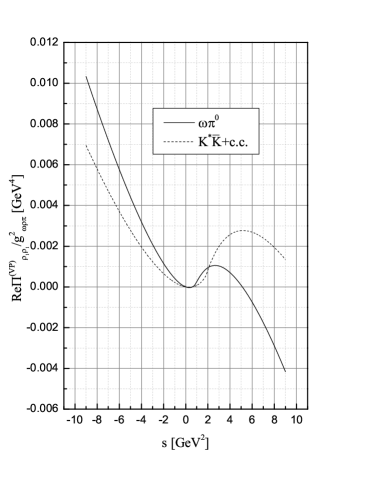
Figure 1: The dependence of Re$\Pi^{(VP)}_{\rho_{1}\rho_{1}}(s)/g^{2}_{\omega\rho_{1}\pi}$ on energy squared; $s_{0}=0.09$ GeV².

The function $G^{(VP)}(s)$ [Eq. (20)] necessary for the evaluation of the nondiagonal polarization operator due to the VP loop is

$$G^{(VP)}(s)=\frac{s^{2}}{48\pi^{2}}\left(\frac{4m_{V}m_{P}}{m_{+}m_{-}}\right)^{3}I^{(VP)}(s),$$ (30)

where

$$I^{(VP)}(s) = \left\{\frac{s^{3}}{16}+\frac{m^{2}_{+}}{4m_{V}m_{P}}(s-m^{2}_{-})\left[\frac{3s^{2}}{8}-\frac{m^{2}_{+}s(s-m^{2}_{-})}{8m_{V}m_{P}}-\left(\frac{m_{+}m_{-}}{4m_{V}m_{P}}\right)^{2}(m^{2}_{+}-s)(s-m^{2}_{-})\right]\right\}\times$$ (31)

$$\frac{1}{2s^{3}}\ln\frac{m_{V}}{m_{P}}+\frac{m_{+}m_{-}}{4m_{V}m_{P}s^{3}}\left\{\frac{s^{2}m^{2}_{-}}{4m_{V}m_{P}}\left[\frac{s}{24}+\frac{m^{2}_{+}(s-m^{2}_{-})}{16m_{V}m_{P}}+\frac{sm^{2}_{-}}{24m_{V}m_{P}}\right]-\frac{s^{3}}{16}-\frac{sm^{2}_{+}(s-m^{2}_{-})}{4m_{V}m_{P}}\right.\times$$

$$\left.\left[\frac{3s}{8}-\frac{m^{2}_{+}(s-m^{2}_{-})}{8m_{V}m_{P}}\right]\right\}+\left(\frac{m_{+}m_{-}}{4m_{V}m_{P}s}\right)^{3}\left|(s-m^{2}_{+})(s-m^{2}_{-}\right|^{3/2}\times$$

$$\left[\frac{1}{2}\theta(m^{2}_{-}-s)\ln\frac{\sqrt{m^{2}_{+}-s}+\sqrt{m^{2}_{-}-s}}{\sqrt{m^{2}_{+}-s}-\sqrt{m^{2}_{-}-s}}+\theta(s-m^{2}_{-})\theta(m^{2}_{+}-s)\arctan\sqrt{\frac{s-m^{2}_{-}}{m^{2}_{+}-s}}+\right.$$

$$\left.\frac{1}{2}\theta(s-m^{2}_{+})\left(i\pi-\ln\frac{\sqrt{s-m^{2}_{-}}+\sqrt{s-m^{2}_{+}}}{\sqrt{s-m^{2}_{-}}-\sqrt{s-m^{2}_{+}}}\right)\right].$$

The dependence of Re$\Pi^{(\omega\pi)}_{\rho_{1}\rho_{2}}/g_{\omega\rho_{1}\pi}g_{\omega\rho_{2}\pi}$ on $s$ is shown in Fig. 2.

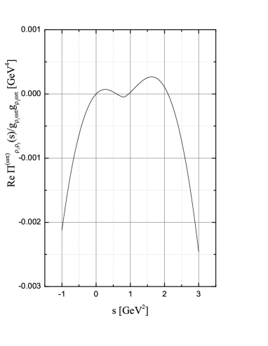
Figure 2: The dependence of Re$\Pi^{(\omega\pi)}_{\rho_{1}\rho_{2}}(s)/g_{\omega\rho_{1}\pi}g_{\omega\rho_{2}\pi}$ on energy squared in case of $m_{\rho_{1}}=770$ MeV and $m_{\rho_{2}}=1450$ MeV.

II.3 Axial vector-pseudoscalar loop

The axial vector-pseudoscalar meson state AP$=a_{1}(1260)\pi$ is considered to be one of the states contributing to the four-pion production amplitude pdg . For soft pions, when taking into account the requirements of chiral symmetry, this amplitude and the corresponding partial width, are very complicated ach00a ; ach00b ; ach08a ; ach08b ; czyz08 ; czyz01 ; ecker89 . This prevents one from using the dispersion relation to obtain the contribution of the four-pion state to the polarization operator of the state $\rho_{i}$. Hence, in the present work, the simplest $a_{1}\pi$ dominance model of the four-pion cmd4pi production is used: $e^{+}e^{-}\to\rho_{i}\to a_{1}\pi\to 4\pi$. The amplitude of the transition $\rho_{i}\to a_{1}\pi$ is chosen in the simplest form

$$A(\rho_{iq}\to a_{1k}\pi_{p}) = g_{\rho_{i}a_{1}\pi}[(\epsilon_{a_{1}}\epsilon_{\rho_{i}})(kq)-$$ (32)

$$(\epsilon_{a_{1}}q)(\epsilon_{\rho_{i}}k)],$$

where $q$, $k$, and $p$ are, respectively, the four-momenta of the mesons $\rho_{i}$, $a_{1}$, and $\pi$, while $\epsilon_{a_{1}}$ and $\epsilon_{\rho_{i}}$ denote the polarization four-vectors of $a_{1}$ and $\rho_{i}$. The expression (32) is chosen on the grounds that it is explicitly transverse in the $\rho_{i}$ leg.

The diagonal polarization operators due to the AP loop are represented in the form

$$\Pi_{\rho_{i}\rho_{i}}^{(AP)}=g^{2}_{\rho_{i}AP}\Pi^{(AP)},$$ (33)

where the quantity $\Pi^{(AP)}\equiv\Pi^{(AP)}(s,m_{\rho_{i}},m_{A},m_{P})$ is calculated from the dispersion relation

$$\frac{\Pi^{(AP)}}{s} = \frac{1}{48\pi^{2}}\int_{(m_{A}+m_{P})^{2}}^{\infty}\frac{q_{AP}(s^{\prime},m_{A},m_{P})}{(s^{\prime})^{3/2}(s^{\prime}-s-i\varepsilon)}\times$$ (34)

$$[(s^{\prime}+m^{2}_{A}-m^{2}_{P})^{2}+2s^{\prime}m^{2}_{A}]\times$$

$$\left(\frac{s_{0}+m^{2}_{\rho_{i}}}{s_{0}+s^{\prime}}\right)ds^{\prime},$$

where the expression

$$\Gamma_{\rho_{i}\to AP}(s) = \frac{g^{2}_{\rho_{i}AP}}{48\pi s}\left[(s+m^{2}_{A}-m^{2}_{P})^{2}+2sm^{2}_{A}\right]\times$$ (35)

$$q_{AP}(s,m_{A},m_{P})\left(\frac{s_{0}+m^{2}_{\rho_{i}}}{s_{0}+s}\right)$$

for the $\rho_{i}\to AP$ decay width found from the effective vertex Eq. (32) is inserted into the integrand of the dispersion relation. The result of integration is represented in the form

$$\Pi^{(AP)} = \frac{s}{96\pi^{2}}\left(\frac{m_{-}}{m_{+}}\right)^{3}\frac{m^{2}_{\rho_{i}}+s_{0}}{s+s_{0}}\left[J(s)-\right.$$ (36)

$$\left.{\rm Re}J(m^{2}_{\rho_{i}})\frac{s+s_{0}}{m^{2}_{\rho_{i}}+s_{0}}\right],$$

where $m_{\pm}=m_{A}\pm m_{P}$,

$$J(s) = sf(s)\left[\left(\frac{m^{2}_{+}}{s}-1\right)^{2}+\frac{2m_{A}}{m_{-}}\times\right.$$ (37)

$$\left.\left(2+\frac{m_{A}}{m_{-}}\right)\left(\frac{m^{2}_{+}}{s}-1\right)+6\frac{m^{2}_{A}}{m^{2}_{-}}\right]-$$

$$s_{0}f_{2}\left[\left(\frac{m^{2}_{+}}{s_{0}}+1\right)^{2}-\frac{2m_{A}}{m_{-}}\times\right.$$

$$\left.\left(2+\frac{m_{A}}{m_{-}}\right)\left(\frac{m^{2}_{+}}{s_{0}}+1\right)+6\frac{m^{2}_{A}}{m^{2}_{-}}\right].$$

The function $f(s)$ looks as

$$f(s) = \frac{m_{+}}{sm_{-}}\left\{(s-m^{2}_{-})\frac{m_{+}}{m_{-}}\ln\frac{m_{A}}{m_{P}}-s\left(\frac{m^{2}_{+}-m^{2}_{-}}{2m_{+}m_{-}}\ln\frac{m_{A}}{m_{P}}-1\right)+\sqrt{|(s-m^{2}_{+})(s-m^{2}_{-})|}\times\right.$$ (38)

$$\left.\left[\theta(m^{2}_{-}-s)\ln\frac{\sqrt{m^{2}_{+}-s}+\sqrt{m^{2}_{-}-s}}{\sqrt{m^{2}_{+}-s}+\sqrt{m^{2}_{-}-s}}-2\theta(s-m^{2}_{-})\theta(m^{2}_{+}-s)\arctan\sqrt{\frac{s-m^{2}_{-}}{m^{2}_{+}-s}}-\right.\right.$$

$$\left.\left.\theta(s-m^{2}_{+})\left(-i\pi+\ln\frac{\sqrt{s-m^{2}_{-}}+\sqrt{s-m^{2}_{+}}}{\sqrt{s-m^{2}_{-}}-\sqrt{s-m^{2}_{+}}}\right)\right]\right\},$$

and

$$f_{2} = -\frac{m_{+}}{m_{-}}\left[\frac{m_{+}}{m_{-}}\left(1+\frac{m^{2}_{-}}{s_{0}}\right)\left(\ln\frac{m_{A}}{m_{P}}-\frac{2m_{-}}{m_{+}}\sqrt{\frac{m^{2}_{+}+s_{0}}{m^{2}_{-}+s_{0}}}\tanh^{-1}\sqrt{\frac{m^{2}_{-}+s_{0}}{m^{2}_{+}+s_{0}}}\right)-\frac{m^{2}_{+}-m^{2}_{-}}{2m_{+}m_{-}}\ln\frac{m_{A}}{m_{P}}+1\right]$$ (39)

The dependence of Re$\Pi^{(AP)}_{\rho_{1}\rho_{1}}(s)$ on energy squared is shown in Fig. 3.

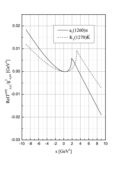
Figure 3: The dependence of Re$\Pi^{(AP)}_{\rho_{1}\rho_{1}}(s)$ on energy squared $s$ for the $AP=a_{1}(1260)\pi$ and $AP=K_{1}(1270)\bar{K}$ loops demonstrating discontinuity of $\frac{d{\rm Re}\Pi^{(AP)}}{ds}$ at $s=(m_{A}+m_{P})^{2}$. The parameters are $m_{\rho}=777$ MeV, $m_{a_{1}}=1230$ MeV, $m_{K_{1}}=1270$ MeV, $s_{0}=0.09$ GeV².

The function $G^{(AP)}(s)$ [Eq. (20)] necessary for evaluation of the nondiagonal polarization operator due to the AP loop is

$$G^{(AP)}(s)=\frac{s^{2}}{48\pi^{2}}\left(\frac{4m_{A}m_{P}}{m_{+}m_{-}}\right)^{3}I^{(AP)}(s),$$ (40)

where

$$I^{(AP)}(s) = \left\{\frac{1}{16}+\frac{m^{2}_{-}}{32m_{A}m_{P}}\left(\frac{m^{2}_{+}}{s}-1\right)+\frac{m_{A}+2m_{-}}{16m_{P}}+\frac{1}{2}\left(\frac{m_{+}m_{-}}{4m_{A}m_{P}}\right)^{2}\left(\frac{m^{2}_{+}}{s}-1\right)\left(1-\frac{m^{2}_{-}}{s}\right)-\right.$$ (41)

$$\left.\frac{m^{2}_{-}(m_{A}+2m_{P})}{16m_{A}m^{2}_{P}}-\frac{3m^{2}_{-}}{16m^{2}_{P}}+\frac{m^{2}_{+}}{4m_{A}m_{P}}\left(1-\frac{m^{2}_{-}}{s}\right)\left[\left(\frac{m^{2}_{-}}{4m_{A}m_{P}}\right)^{2}\left(\frac{m^{2}_{+}}{s}-1\right)^{2}+\right.\right.$$

$$\left.\left.\frac{m^{2}_{-}}{2m_{A}m_{P}}\left(\frac{m^{2}_{+}}{s}-1\right)+\frac{3m^{2}_{-}}{8m^{2}_{P}}\right]\right\}\times\frac{1}{2}\ln\frac{m_{A}}{m_{P}}+\frac{m_{+}m_{-}}{4m_{A}m_{P}}\left\{\frac{1}{6}\left(\frac{m^{2}_{+}}{4m_{A}m_{P}}\right)^{2}+\frac{m^{2}_{-}}{4m_{A}m_{P}}\left[\frac{1}{24}-\right.\right.$$

$$\left.\left.\frac{m^{2}_{-}}{16m_{A}m_{P}}\left(\frac{m^{2}_{+}}{s}-1\right)-\frac{m_{A}+2m_{-}}{8m_{P}}\right]-\frac{1}{16}+\frac{3m^{2}_{-}}{32m_{A}m_{P}}\left(\frac{m^{2}_{+}}{s}-1\right)+\frac{3(m_{A}+2m_{-})}{16m_{P}}-\right.$$

$$\left.\frac{1}{2}\left(\frac{m_{+}m_{-}}{4m_{A}m_{P}}\right)^{2}\left(\frac{m^{2}_{+}}{s}-1\right)\left(1-\frac{m^{2}_{-}}{s}\right)-\frac{m^{2}_{+}(m_{A}+2m_{P})}{16m_{A}m^{2}_{P}}\left(1-\frac{m^{2}_{-}}{s}\right)+\frac{3m^{2}_{-}}{16m^{2}_{P}}+\frac{1}{s}\times\right.$$

$$\left.\left[\left(\frac{m^{2}_{-}}{4m_{A}m_{P}}\right)^{2}\left(\frac{m^{2}_{+}}{s}-1\right)^{2}+\frac{m^{2}_{-}}{2m_{A}m_{P}}\left(\frac{m^{2}_{+}}{s}-1\right)+\frac{3m^{2}_{-}}{8m^{2}_{P}}\right]\left|(s-m^{2}_{-})(s-m^{2}_{+}\right|^{1/2}\times\right.$$

$$\left.\left[\frac{1}{2}\theta(m^{2}_{-}-s)\ln\frac{\sqrt{m^{2}_{+}-s}+\sqrt{m^{2}_{-}-s}}{\sqrt{m^{2}_{+}-s}-\sqrt{m^{2}_{-}-s}}-\theta(s-m^{2}_{-})\theta(m^{2}_{+}-s)\arctan\sqrt{\frac{s-m^{2}_{-}}{m^{2}_{+}-s}}+\right.\right.$$

$$\left.\left.\frac{1}{2}\theta(s-m^{2}_{+})\left(i\pi-\ln\frac{\sqrt{s-m^{2}_{-}}+\sqrt{s-m^{2}_{+}}}{\sqrt{s-m^{2}_{-}}-\sqrt{s-m^{2}_{+}}}\right)\right]\right\}.$$

The dependence of Re$\Pi^{(a_{1}\pi)}_{\rho_{1}\rho_{2}}/g_{a_{1}\rho_{1}\pi}g_{a_{1}\rho_{2}\pi}$ on $s$ is shown in Fig. 4.

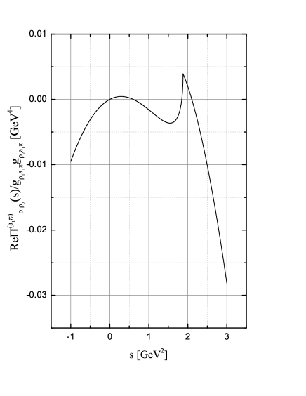
Figure 4: The dependence of Re$\Pi^{(a_{1}\pi)}_{\rho_{1}\rho_{2}}(s)/g_{a_{1}\rho_{1}\pi}g_{a_{1}\rho_{2}\pi}$ on energy squared in case of $m_{\rho_{1}}=770$ MeV and $m_{\rho_{2}}=1450$ MeV.

II.4 Polarization operators used in fits

Although the nature of the higher resonances $\rho(1450)$, $\rho(1700)$, … is the subject of current and future studies, the quark-antiquark model relations between their coupling constants are assumed:

$$g_{\rho_{i}K^{\ast}K} = \frac{1}{2}g_{\rho_{i}\omega\pi},$$

$$g_{\rho_{i}K_{1}(1270)K} = \frac{1}{2}g_{\rho_{i}a_{1}(1260)\pi}.$$ (42)

Polarization operators which take into account three channels described above are the following. The full diagonal polarization operators are

$$\Pi_{\rho_{i}\rho_{i}}=\Pi^{(PP)}_{\rho_{i}\rho_{i}}+\Pi^{(VP)}_{\rho_{i}\rho_{i}}+\Pi^{(AP)}_{\rho_{i}\rho_{i}}.$$ (43)

In the present work, we take into account the following analytically calculated loops. First, we use the PP $\pi^{+}\pi^{-}$ and $K^{+}K^{-}+K^{0}\bar{K}^{0}$ loops,

$$\Pi^{(PP)}_{\rho_{i}\rho_{i}} = g^{2}_{\rho_{i}\pi\pi}\left[\Pi^{(PP)}(s,m_{\rho_{i}},m_{\pi})+\right.$$ (44)

$$\left.\frac{1}{2}\Pi^{(PP)}(s,m_{\rho_{i}},m_{K})\right],$$

with $\Pi^{(PP)}$ given by Eq. (22). Second, we use the VP $\omega\pi^{0}$ and $K^{\ast}\bar{K}^{+}\bar{K}^{\ast}K$ loops,

$$\Pi^{(VP)}_{\rho_{i}\rho_{i}} = g^{2}_{\rho_{i}\omega\pi}\left[\Pi^{(VP)}(s,m_{\rho_{i}},m_{\omega},m_{\pi})+\right.$$ (45)

$$\left.\Pi^{(VP)}(s,m_{\rho_{i}},m_{K^{\ast}},m_{K})\right],$$

with $\Pi^{(VP)}\equiv\Pi^{(VP)}(s,m_{\rho_{i}},m_{V},m_{P})$ given by Eq. (28). Third, we use the AP $a_{1}(1260)^{+}\pi^{-}+a_{1}(1260)^{-}\pi^{+}$, $K_{1}(1270)\bar{K}+$ c.c. loops,

$$\Pi^{(AP)}_{\rho_{i}\rho_{i}} = 2g^{2}_{\rho_{i}a_{1}\pi}\left[\Pi^{(AP)}(s,m_{\rho_{i}},m_{a_{1}},m_{\pi})+\right.$$ (46)

$$\left.\frac{1}{2}\Pi^{(AP)}(s,m_{\rho_{i}},m_{K_{1}(1270)},m_{K})\right],$$

with $\Pi^{(AP)}\equiv\Pi^{(AP)}(s,m_{\rho_{i}},m_{A},m_{P})$ given by Eq. (36).

Similar expressions are used for the nondiagonal polarization operators,

$$\Pi_{\rho_{i}\rho_{j}}=\Pi^{(PP)}_{\rho_{i}\rho_{j}}+\Pi^{(VP)}_{\rho_{i}\rho_{j}}+\Pi^{(AP)}_{\rho_{i}\rho_{j}},$$ (47)

where

$$\Pi^{(PP)}_{\rho_{i}\rho_{j}} = g_{\rho_{i}\pi\pi}g_{\rho_{j}\pi\pi}\left[\Pi_{\rho_{i}\rho_{j}}(s,m_{\rho_{i}},m_{\rho_{j}},m_{\pi},m_{\pi})+\frac{1}{2}\Pi_{\rho_{i}\rho_{j}}(s,m_{\rho_{i}},m_{\rho_{j}},m_{K},m_{K})\right],$$

$$\Pi^{(VP)}_{\rho_{i}\rho_{j}} = g_{\rho_{i}\omega\pi}g_{\rho_{j}\omega\pi}\left[\Pi_{\rho_{i}\rho_{j}}(s,m_{\rho_{i}},m_{\rho_{j}},m_{\omega},m_{\pi})+\Pi_{\rho_{i}\rho_{j}}(s,m_{\rho_{i}},m_{\rho_{j}},m_{K^{\ast}},m_{K})\right],$$

$$\Pi^{(AP)}_{\rho_{i}\rho_{j}} = 2g_{\rho_{i}a_{1}\pi}g_{\rho_{j}a_{1}\pi}\left[\Pi_{\rho_{i}\rho_{j}}(s,m_{\rho_{i}},m_{\rho_{j}},m_{a_{1}},m_{\pi})+\frac{1}{2}\Pi_{\rho_{i}\rho_{j}}(s,m_{\rho_{i}},m_{\rho_{j}},m_{K_{1}},m_{K})\right],$$ (48)

with $\Pi_{\rho_{i}\rho_{j}}(s,m_{\rho_{i}},m_{\rho_{j}},m_{a},m_{b})$ given by Eq. (19) in which the corresponding $G^{(ab)}(s)$ are given in Eqs. (24), (30), and (40).

III Quantities for comparison with the data

The following reactions are considered in the present work:

$$e^{+}e^{-}\to\pi^{+}\pi^{-},$$ (49)

$$e^{+}e^{-}\to\omega\pi^{0},$$ (50)

and

$$e^{+}e^{-}\to\pi^{+}\pi^{-}\pi^{+}\pi^{-}.$$ (51)

The justification of the restriction to these reactions are given in Introduction and below in Sec. IV. Let us turn to the working expressions necessary for the comparison with the experimental data.

III.1 $\pi^{+}\pi^{-}$ production

In the present case, the relevant quantity is the so-called bare cross section of the reaction (49):

$$\sigma_{\rm bare}=\frac{8\pi\alpha^{2}}{3s^{5/2}}|F_{\pi}(s)|^{2}q^{3}_{\pi}(s)\left[1+\frac{\alpha}{\pi}a(s)\right],$$ (52)

where $F_{\pi}(s)$ is the pion form factor Eq. (11), the quantity $a(s)$ takes into account the radiation by the final pions, and $\alpha=1/137$ is the fine-structure constant. The necessary discussion concerning the quantities in Eq. (52) are given elsewhere ach11 .

III.2 $\omega\pi^{0}$ production

The cross section of the reaction $e^{+}e^{-}\to\omega\pi^{0}$ is taken in the form

$$\sigma_{e^{+}e^{-}\to\omega\pi^{0}} = \frac{4\pi\alpha^{2}}{3s^{3/2}}\left|A_{e^{+}e^{-}\to\omega\pi^{0}}\right|^{2}\times$$ (53)

$$q^{3}_{\omega\pi}(s,m_{\omega},m_{\pi}),$$

where $q_{\omega\pi}$ is given by Eq. (27),

$$A_{e^{+}e^{-}\to\omega\pi^{0}} = (g_{\gamma\rho_{1}},g_{\gamma\rho_{2}},g_{\gamma\rho_{3}},\cdots)G^{-1}\times$$ (58)

$$\left(\begin{array}[]{c}g_{\rho_{1}\omega\pi}\\ g_{\rho_{2}\omega\pi}\\ g_{\rho_{3}\omega\pi}\\ \cdots\\ \end{array}\right),$$

is the amplitude of the reaction, and the matrix

$$G=\left(\begin{array}[]{cccc}D_{1}&-\Pi_{12}&-\Pi_{13}&\cdots\\ -\Pi_{12}&D_{2}&-\Pi_{23}&\cdots\\ -\Pi_{13}&-\Pi_{23}&D_{3}&\cdots\\ \cdots&\cdots&\cdots\\ \end{array}\right)$$ (59)

is introduced in order to take into account the strong mixing of the resonances $\rho_{i}$ ach11 . Here, $\Pi_{ij}\equiv\Pi_{\rho_{i}\rho_{j}}$ are the polarization operators. See Eqs. (43) and (47). The nondiagonal $i\not=j$ terms describe the mixing. The inverse propagators $D_{i}$ are given by Eq. (14).

III.3 $\pi^{+}\pi^{-}\pi^{+}\pi^{-}$ production

The width of the decay $\rho_{i}\to 2\pi^{+}2\pi^{-}$ in the model (32) is represented in the form

$$\Gamma_{\rho_{i}\to 2\pi^{+}2\pi^{-}}(s)=g^{2}_{\rho_{i}a_{1}\pi}W_{\pi^{+}\pi^{-}\pi^{+}\pi^{-}}(s),$$ (60)

where

$$W_{\pi^{+}\pi^{-}\pi^{+}\pi^{-}}(s) = \frac{1}{12\pi}\int_{(3m_{\pi})^{2}}^{(\sqrt{s}-m_{\pi})^{2}}\rho_{a_{1}}(m^{2})\times$$ (61)

$$\left[\frac{(s+m^{2}-m^{2}_{\pi})^{2}}{2s}+m^{2}\right]\times$$

$$q_{a_{1}\pi}(s,m^{2},m^{2}_{\pi})dm^{2}$$

and $q_{a_{1}\pi}$ is given by Eq. (27). The function

$$\rho_{a_{1}}(m^{2})=\frac{m_{a_{1}}\Gamma_{a_{1}}/\pi}{(m^{2}-m^{2}_{a_{1}})^{2}+m^{2}_{a_{1}}\Gamma^{2}_{a_{1}}}$$ (62)

is introduced to take into account the large width of the intermediate $a_{1}$ resonance in a minimal way, by taking the limit of the fixed $a_{1}$ width. The mass and width of $a_{1}(1260)$ are determined from fitting the data on the reaction $e^{+}e^{-}\to\pi^{+}\pi^{-}\pi^{+}\pi^{-}$.

The cross section of the reaction $e^{+}e^{-}\to\pi^{+}\pi^{-}\pi^{+}\pi^{-}$ is represented in the form

$$\sigma_{\pi^{+}\pi^{-}\pi^{+}\pi^{-}} = \frac{(4\pi\alpha)^{2}}{3s^{3/2}}\left|(g_{\gamma\rho_{1}},g_{\gamma\rho_{2}},g_{\gamma\rho_{3}},\cdots)G^{-1}\left(\begin{array}[]{c}g_{\rho_{1}a_{1}\pi}\\ g_{\rho_{2}a_{1}\pi}\\ g_{\rho_{3}a_{1}\pi}\\ \cdots\\ \end{array}\right)\right|^{2}W_{\pi^{+}\pi^{-}\pi^{+}\pi^{-}}(s)$$ (67)

with $W_{\pi^{+}\pi^{-}\pi^{+}\pi^{-}}(s)$ given by Eq. (61), represents the effective phase-space volume of the four pions via the smearing [Eq. (62)] of the $a_{1}\pi$ phase-space volume. The matrix $G$ is the matrix of inverse propagators, Eq. (59).

IV Results of data fitting

This section is devoted to the presentation of the results of fitting the data on the reactions $e^{+}e^{-}\to\pi^{+}\pi^{-}$, $e^{+}e^{-}\to\omega\pi^{0}$, and $e^{+}e^{-}\to\pi^{+}\pi^{-}\pi^{+}\pi^{-}$. Two possible fitting schemes were used.

• Scheme 1: Three resonances $\rho(770)+\rho(1450)+\rho(1700)$ and the PP loops of pseudoscalar mesons are taken into account ach11 ; ach12 .

When adding the VP- and AP-loop contributions to the pion form factor one should also include the VP and AP final states. These states manifest, respectively, in the reactions $e^{+}e^{-}\to\omega\pi^{0}$ and $e^{+}e^{-}\to\pi^{+}\pi^{-}\pi^{+}\pi^{-}$ which should also be treated in the present framework. Since energies higher than 2 GeV are considered, the third heavy isovector resonance $\rho(2100)$ is added. Hence, the scheme with the resonances $\rho(770)+\rho(1450)+\rho(1700)+\rho(2100)$ and the PP, VP, and AP loops in the polarization operators is used. This is scheme 2:

• Scheme 2. The data on the reactions $e^{+}e^{-}\to\pi^{+}\pi^{-}$ babar , $e^{+}e^{-}\to\omega\pi^{0}$ snd13 , and $e^{+}e^{-}\to\pi^{+}\pi^{-}\pi^{+}\pi^{-}$ bab4pi are fitted separately in the model which takes into account the resonances $\rho(770)+\rho(1450)+\rho(1700)+\rho(2100)$ side by side while allowing for the PP, VP, and AP loops in the polarization operators.

The parameters found from the fitting scheme 2 are listed in Table 1.

Table 1: The resonance parameters found from fitting the data on the reactions $e^{+}e^{-}\to\pi^{+}\pi^{-}$ babar , $e^{+}e^{-}\to\pi^{+}\pi^{-}\pi^{+}\pi^{-}$ bab4pi , and $e^{+}e^{-}\to\omega\pi^{0}$ snd13 , in the fitting scheme 2 (see text). The parameter Re$\Pi^{\prime}_{\omega\rho}$ is responsible for $\omega\rho$ mixing, see Ref. ach11 for more detail. The parameter $g_{\rho_{4}}$ can be found from the sum rule $\frac{g_{\rho_{1}\pi\pi}}{g_{\rho_{1}}}+\frac{g_{\rho_{2}\pi\pi}}{g_{\rho_{2}}}+\frac{g_{\rho_{3}\pi\pi}}{g_{\rho_{3}}}+\frac{g_{\rho_{4}\pi\pi}}{g_{\rho_{4}}}=1$, which provides the correct normalization $F_{\pi}(0)=1$.

parameter	$e^{+}e^{-}\to\pi^{+}\pi^{-}$	$e^{+}e^{-}\to\pi^{+}\pi^{-}\pi^{+}\pi^{-}$	$e^{+}e^{-}\to\omega\pi^{0}$
$m_{\rho_{1}}$[MeV]	$765.6\pm 0.1$	$\equiv 777$	$\equiv 777$
$g_{\rho_{1}\pi\pi}$	$6.336\pm 0.004$	$5.78\pm 0.01$	$6.63\pm 0.03$
$g_{\rho_{1}}$	$4.662\pm 0.002$	$5.66\pm 0.02$	$4.80\pm 0.02$
$g_{\rho_{1}a_{1}\pi}$[GeV-1]	$2.37\pm 0.05$	$0.26\pm 0.02$	$5.61\pm 0.08$
$m_{\omega}$[MeV]	$782.02\pm 0.10$	$\equiv 782.02$	$\equiv 782.02$
Re$\Pi^{\prime}_{\omega\rho}$[GeV2]	$(4.38\pm 0.07)\times 10^{-3}$	$-$	$-$
$m_{\rho_{2}}$[MeV]	$1507\pm 3$	$1122\pm 1$	$1412\pm 6$
$g_{\rho_{2}\pi\pi}$	$-6.01\pm 0.03$	$-5.45\pm 0.03$	$-5.72\pm 0.08$
$g_{\rho_{2}}$	$78\pm 2$	$8.74\pm 0.04$	$21.6\pm.4$
$g_{\rho_{2}\omega\pi}$[GeV-1]	$6.66\pm 0.07$	$38.2\pm 0.2$	$32\pm 2$
$g_{\rho_{2}a_{1}\pi}$[GeV-1]	$1.48\pm 0.11$	$5.61\pm 0.03$	$-1.37\pm 0.15$
$m_{\rho_{3}}$[MeV]	$1831\pm 4$	$1648\pm 1$	$1661\pm 5$
$g_{\rho_{3}\pi\pi}$	$-2.800\pm 0.008$	$3.681\pm 0.005$	$-0.90\pm 0.03$
$g_{\rho_{3}}$	$8.45\pm 0.05$	$4.302\pm 0.005$	$4.90\pm 0.04$
$g_{\rho_{3}\omega\pi}$[GeV-1]	$5.32\pm 0.02$	$0.98\pm 0.02$	$22.0\pm 0.3$
$g_{\rho_{3}a_{1}\pi}$[GeV-1]	$0.41\pm 0.06$	$-1.692\pm 0.005$	$3.1\pm 0.1$
$m_{\rho_{4}}$[MeV]	$2154\pm 15$	$2390\pm 5$	$1969\pm 7$
$g_{\rho_{4}\pi\pi}$	$-1.78\pm 0.03$	$-4.5\pm 0.1$	$-3.11\pm 0.08$
$g_{\rho_{4}\omega\pi}$[GeV-1]	$8.65\pm 0.12$	$11.39\pm 0.05$	$8.19\pm 0.10$
$g_{\rho_{4}a_{1}\pi}$[GeV-1]	$1.63\pm 0.05$	$1.004\pm 0.035$	$-0.91\pm 0.02$
$m_{K_{1}(1270)}$[MeV]	$\equiv 1270$	$1265\pm 1$	$1230\pm 7$
$m_{a_{1}(1260)}$[MeV]	$\equiv 1230$	$1132\pm 1$	$1268\pm 4$
$\Gamma_{a_{1}(1260)}$[MeV]	$-$	$1028\pm 3$	$-$
$s_{0}$[GeV]2	$4.33\pm 0.03$	$0.00037\pm 0.00001$	$0.09\pm 0.03$
$\chi^{2}/N_{\rm d.o.f}$	335/316	400/59	43/20

Let us comment on each of the mentioned channels.

IV.1 Fitting $e^{+}e^{-}\to\pi^{+}\pi^{-}$ data

When fitting the data on the reaction $e^{+}e^{-}\to\pi^{+}\pi^{-}$ at energies $\sqrt{s}\leq 1$ GeV in our previous publication ach11 ; ach12 ; ach13 , the fitting scheme 1 was used. There, the restriction to the PP loop was justifiable because of rather low energies under consideration. Using the resonance parameters found from fitting the data in the time-like region, the pion form factor $F_{\pi}(s)$ in the space-like region $s<0$ was calculated up to $-s=Q^{2}=0.2$ GeV² and compared with the NA7 data amendolia . A comparison with the data bebek ; horn ; tadev in the wider range up to $-s=Q^{2}=10$ GeV² was made in Ref. ach13 . In the present work, we give the corresponding plot in Fig. 5 for the sake of completeness. The continuation to the space-like domain in the fitting scheme 2 is discussed below.

Figure 5: The pion form factor squared in the space-like region $s<0$ evaluated using the resonance parameters of the Table I in Ref. ach11 , the BaBaR column, the fitting scheme 1. See text. The experimental data are: NA7 amendolia , Bebek et al. bebek , Horn et al. horn , Tadevosyan et al.tadev .

The cross section of the reaction $e^{+}e^{-}\to\pi^{+}\pi^{-}$ fitted in the scheme 2 is shown in Fig. 6. As for the $\rho(770)$ resonance parameters are concerned, one can observe that in comparison with the fit in the scheme 1 ach11 ; ach12 ; ach13 , the bare mass of the resonance $\rho_{1}$ determined in the scheme 2 in the sensitive channel $e^{+}e^{-}\to\pi^{+}\pi^{-}$ is typically lower. Compare Table 1 here and the Table I in, e.g., Ref. ach11 . The same concerns the coupling constant $g_{\rho_{1}}$ which parametrizes the leptonic decay width (13). The coupling constant $g_{\rho_{1}\pi\pi}$ in the scheme 2 is greater than in the scheme 1. The above distinction can be qualitatively explained by the effect of renormalization of the coupling constants described in Ref. ach11 . Indeed, as was shown in Ref. ach11 , the renormalization results in the substitutions

$$g_{\rho_{1}\pi\pi} \to Z_{\rho}^{-1/2}g_{\rho_{1}\pi\pi},$$

$$g_{\rho_{1}} \to Z_{\rho}^{1/2}g_{\rho_{1}},$$ (68)

where

$$Z_{\rho}=1+\frac{d{\rm Re}\Pi_{\rho_{1}\rho_{1}}(s)}{ds}\left|{}_{s=m^{2}_{\rho_{1}}}\right..$$ (69)

Equation (68) means that the bare $g_{\rho_{1}\pi\pi}$ obtained from the fit is related to the ”physical” one obtained from the visible peak, upon multiplying by $Z^{1/2}_{\rho}$, while the opposite is true for $g_{\rho_{1}}$. The contributions of the VP loop to $d{\rm Re}\Pi_{\rho_{1}\rho_{1}}/ds$ near $s=m^{2}_{\rho_{1}}$, as is observed from Fig. 1, is positive and exceed the negative contribution from the PP loop, see Fig. 7 in Ref. ach11 . The same is true for the AP loop. As a result, one has $Z_{\rho}>1$.

Although the energy behavior of the cross section up to $\sqrt{s}=1.7$ GeV is described in the adopted model, including the dip near 1.5 GeV, one can see that the structure in the interval 2-2.5 GeV demands, in all appearance, additional $\rho$-like resonances and/or intermediate states in the loops. We tried to include the contribution of $K_{1}(1400)\bar{K}$+c.c. states coupled solely to the resonance $\rho_{4}$, with the fitted coupling constant $g_{\rho_{4}K_{1}(1400)K}$ and mass $m_{K_{1}(1400)}$. This slightly improves the agreement in the interval $1.75<\sqrt{s}<2$ GeV but occurs at the expense of adding two additional free parameters and does not result in reproducing the peak near $\sqrt{s}=2.3$ GeV.

Figure 6: The cross section of the reaction $e^{+}e^{-}\to\pi^{+}\pi^{-}$. The data are from Ref. babar , and the curve is drawn using the resonance parameters of scheme 2. The $\rho-\omega$ resonance region is shown in the insert.

The continuation to the space-like region $s<0$ with the resonance parameters obtained in the region $s>4m^{2}_{\pi}$ in fitting scheme 2 with the VP and AP loops added, results in unwanted behavior of $F_{\pi}(s)$, see Fig. 7. Specifically, the curve goes through experimental points amendolia up to $s=-0.2$ GeV², but at larger values of $-s=Q^{2}$ one encounters infinities arising from the the Landau poles due to the VP and AP loops.

Figure 7: The same as in Fig. 5, but with the resonance parameters obtained in fitting scheme 2 (see text).

As was pointed out in Ref. ach11 , the Landau pole is present even in the case of the PP loop, but its position is at $\sqrt{Q^{2}}\approx 90$ GeV, that is, it is far from accessible momentum transfers. In the case of the VP and AP loops the Landau poles appear in the region accessible to existing experiments bebek ; horn ; tadev , because of the large magnitude of the coupling constant $g_{\rho_{1}\omega\pi}=13.2$ GeV^-1 fn1 .

An important feature of the new expression for the pion form factor obtained in Ref. ach11 which was not mentioned there is that it does not require ach13 the commonly accepted Blatt-Weisskopf centrifugal factor blatt

$$C_{\pi}(k)=\frac{1+R^{2}_{\pi}k^{2}_{R}}{1+R^{2}_{\pi}k^{2}},$$

in the expression for $\Gamma_{\rho\pi\pi}(s)$ pdg . Here $k$ is the pion momentum at some arbitrary energy while $k_{R}$ is its value at the resonance energy. The fact is that the usage of $R_{\pi}$-dependent centrifugal barrier penetration factor in particle physics – for example, in the case of the $\rho(770)$ meson pdg , results in the overlooked problem. Indeed, the meaning of $R_{\pi}$ is that this quantity is the characteristic of the potential (or the $t$-channel exchange in field theory) resulting in the phase $\delta_{\rm bg}$ of the potential scattering in addition to the resonance phase blatt . For example, in case of the $P$-wave scattering in the potential

$$U(r)=G\delta(r-R_{\pi})$$

where the resonance scattering is possible, the background phase is

$$\delta_{\rm bg}=-R_{\pi}k+\arctan(R_{\pi}k).$$

At the usual value of $R_{\pi}\sim 1$ fm, $\delta_{\rm bg}$ is not small. However, in the $\rho$-meson region, the background phase shift $\delta_{\rm bg}$ is negligible and the phase shift $\delta^{1}_{1}$ is completely determined by the resonance; see Fig. 8 in Ref. ach11 . Therefore, the descriptions of the hadronic resonance distributions which invoke the parameter $R_{\pi}$, have a dubious character.

IV.2 Fitting $e^{+}e^{-}\to\pi^{+}\pi^{-}\pi^{+}\pi^{-}$ data

The dynamics of the reaction $e^{+}e^{-}\to\pi^{+}\pi^{-}\pi^{+}\pi^{-}$ at energies $\sqrt{s}<1$ GeV is determined by the chiral-invariant mechanisms whose amplitudes are too cumbersome to include into the loop integrations for the purposes of fits. Hence we restrict ourselves by the energy range $1<\sqrt{s}<3$ GeV dominated by the $\rho(1450)$, $\rho(1450)$, … $s$-channel production mechanism. The energy dependence of the $e^{+}e^{-}\to\pi^{+}\pi^{-}\pi^{+}\pi^{-}$ reaction cross section is shown in Fig. 8. One can see that at energies $\sqrt{s}>1.75$ GeV the chosen scheme with three heavier rho-like resonances $\rho_{2,3,4}$ cannot reproduce the structures in the measured cross section such as the bizarre sharp turn in the energy behavior followed by fluctuations. As in the case of the reaction $e^{+}e^{-}\to\pi^{+}\pi^{-}$, the contributions of the AP loops $a_{1}(1260)\pi$ and $K_{1}(1270)\bar{K}$+c.c. coupled to all $\rho_{i}$ resonances ($i=1,2,3,4$) were invoked to explain the features above 1.75 GeV. The structures remain unexplained.

Figure 8: The cross section of the reaction $e^{+}e^{-}\to\pi^{+}\pi^{-}\pi^{+}\pi^{-}$. The data are bab4pi , the curve is drawn using the resonance parameters of the scheme 2.

As is seen from Table 1, the coupling constants $g_{\rho_{1}}$ and $g_{\rho_{1}\pi\pi}$ of the $\rho(770)$ meson found from fitting this channel, differ from those found from fitting the $\pi^{+}\pi^{-}$ one. Furthermore, the coupling constant $g_{\rho_{1}a_{1}\pi}$ found from fitting the channel $e^{+}e^{-}\to\pi^{+}\pi^{-}\pi^{+}\pi^{-}$, is suppressed in comparison with the naive chiral-symmetry estimate $g_{a_{1}\to\rho_{1}\pi}\sim 1/2f_{\pi}\sim 5$ GeV^-1 ach05 , where $f_{\pi}=92.4$ MeV is the pion decay constant. We believe that this difference is an artifact of the oversimplified $a_{1}\pi$ model and the price that comes with the possibility of using the analytical calculation of the VP and AP loops to simulate the contributions of the multiparticle meson states in polarization operators fn3 . In the meantime, the coupling constants $g_{\rho_{1}a_{1}\pi}\approx 2.4$ and 5.6 GeV^-1 found from fitting the $e^{+}e^{-}\to\pi^{+}\pi^{-}$ and $e^{+}e^{-}\to\omega\pi^{0}$ channels respectively, look sensible. For comparison, the estimates of $g_{\rho_{1}a_{1}\pi}$ in the model adopted in the present work are $\sim 6$ GeV^-1 and $\sim 4$ GeV^-1, as extracted from $\Gamma_{a_{1}}\approx 0.6$ GeV and 0.3 GeV pdg , respectively. Note also that $\Gamma_{a_{1}\to\rho\pi\to 3\pi}\sim 1$ GeV when evaluated in the generalized hidden local symmetry chiral model for $m_{a_{1}}\approx 1.2$ GeV ach05 . The width of the visible peak in Fig. 8 is about 0.44 GeV which should be compared with $\Gamma_{\rho_{3}}(\sqrt{s}=m_{\rho_{3}})=0.45$ GeV evaluated with the $\pi^{+}\pi^{-}\pi^{+}\pi^{-}$ column of the Table 1.

IV.3 Fitting $e^{+}e^{-}\to\omega\pi^{0}$ data

Quite recently, new data on the reaction $e^{+}e^{-}\to\omega\pi^{0}$ in the decay mode $\omega\to\pi^{0}\gamma$ were published by SND collaboration snd13 . They are analyzed with the fitting scheme 2. The resulting curve calculated with the parameters cited in the Table 1 is shown in Fig. 9.

Figure 9: The cross section of the reaction $e^{+}e^{-}\to\omega\pi^{0}\to\pi^{0}\pi^{0}\gamma$. The data are SND13 snd13 . The curve is drawn using the resonance parameters of the scheme 2.

V Conclusion

The main purpose of the present work is to describe the pion electromagnetic form factor $F_{\pi}(s)$ up to the $J/\psi$ energy range, using the expression obtained in Ref. ach11 . This expression, when restricted to the PP loops in polarization operators, permits a good description of the data of SND, CMD-2, KLOE, and $BABAR$ on $\pi^{+}\pi^{-}$ production in $e^{+}e^{-}$ annihilation at $\sqrt{s}<1$ GeV, describes the scattering kinematical domain up to $-s=Q^{2}=10$ GeV², and does not contradict the data on $\pi\pi$ scattering phase $\delta^{1}_{1}$. The goal of extending the description to the energies up to 3 GeV in the time-like domain was reached by the inclusion of the VP- and AP-loops in addition to the PP ones. These loops contain the couplings of the $\rho$-like resonances with the VP- and AP-states and generate, in turn, the final states $\omega\pi^{0}$ and $\pi^{+}\pi^{-}\pi^{+}\pi^{-}$ in $e^{+}e^{-}$ annihilation. Therefore, consistency demands the treatment of these final states as well. As is shown in the present work, the energy behavior of the cross sections of the reactions $e^{+}e^{-}\to\omega\pi^{0}$ and $e^{+}e^{-}\to\pi^{+}\pi^{-}\pi^{+}\pi^{-}$ obtained in the adopted simplified model, does not contradict the data. The statistically poor description of the cross section of the reaction $e^{+}e^{-}\to\pi^{+}\pi^{-}\pi^{+}\pi^{-}$ is, probably, an artifact of the oversimplified model for its amplitude which ignores both the requirements of the chiral symmetry at lower energies and a complicated intermediate state at higher energies. The proper treatment of the reaction $e^{+}e^{-}\to\pi^{+}\pi^{-}\pi^{+}\pi^{-}$ is beyond the scope of the present work. Nevertheless, we included this poor description for the consistency of the presentation.

One should not wonder at the fact that the masses of heavier $\rho$-like resonances quoted in Table 1 differ from the values quoted in Ref. pdg . In fact, the values in Ref. pdg are only educated guesses, and the masses of heavier $\rho$-like resonances quoted by the Particle Data Group fall into wide intervals; for instance, $m_{\rho_{2}}=1265-1580$ MeV, and $m_{\rho_{3}}=1430-1850$ MeV pdg . Furthermore, the quoted values are usually obtained from fitting the data with the help of the simplest parametrization such as the sum of the Breit-Wigner amplitudes. In the meantime it is known that the residues of the simple pole contributions not necessarily reveal the true nature of the resonances involved in the process ach07a ; ach11a ; ach12a when the mixings and the dynamical effects like the final-state interaction become essential.

The real problem is that the continuation to the space-like domain of the expression for $F_{\pi}(s)$ with the contributions of the VP and AP loops meets the difficulty of encountering the Landau poles. By all appearances, this is the consequence of the chosen parametrization of the vertex form factor which restricts the growth of the partial widths as the energy increase, in a modest way. A stronger suppression could effectively suppress the couplings of rho-like resonances with the VP and AP states and, in turn, push the Landau zeros to higher space-like momentum transfers. This is the topic of a separate study.

We are grateful to M. N. Achasov for numerous discussions which stimulated the present work. This work is supported in part by the Russian Foundation for Basic Research Grant no. 13-02-00039 and the Interdisciplinary project No 102 of the Siberian Division of the Russian Academy of Sciences.

References

- (1) N. N. Achasov and A. A. Kozhevnikov, Phys. Rev. D83, 113005 (2011). Erratum-ibid. D85, 019901 (2012).
- (2) N. N. Achasov and A. A. Kozhevnikov, Nucl.Phys.Proc.Suppl. 225-227, 10 (2012).
- (3) N. N. Achasov and A. A. Kozhevnikov, JETP Letters 96, 559 (2013)[Pis’ma v ZhETF 96, 627 (2012)].
- (4) M. N. Achasov, et al.. J.Exp.Theor.Phys. 101, 1053 (2005); Zh.Eksp.Teor.Fiz. 101, 1201 (2005) [arXiv:hep-ex/0506076v1].
- (5) R. R. Akhmetshin, et al. (CMD-2 Collaboration), Phys.Lett.B648, 28 (2007) [arXiv:hep-ex/0610021v3].
- (6) F. Ambrosino, et al. (KLOE Collaboration), Phys.Lett. B700, 102 (2011)[arXiv:1006.5313].
- (7) B. Aubert, et al. (The BABAR Collaboration), Phys.Rev.Lett.103, 231801 (2009) [arXiv:0908.3589v1].
- (8) N. N. Achasov and A. A. Kozhevnikov, Phys. Rev. D55, 2663 (1997).
- (9) S. R. Amendolia, et al. Nucl.Phys.B277, 168 (1986).
- (10) C. J. Bebek, et al. Phys.Rev.D17, 1693 (1978).
- (11) T. Horn, et al. Phys.Rev.Lett.97,, 192001 (2006).
- (12) V. Tadevosyan, et al. Phys.Rev.C75, 055205 (2007).
- (13) M. N. Achasov, et. al. Phys. Rev. D88, 054013 (2013).
- (14) J. P. Lees, et al. (The BABAR Collaboration), Phys. Rev. D85, 112009 (2012).
- (15) M. Benayoun, P. David, L. DelBuono, and F. Jegerlehner, Eur. Phys. J. C73, 2453 (2013).
- (16) M. Benayoun, P. David, L. DelBuono, and F. Jegerlehner, Eur. Phys. J. C72, 1848 (2012).
- (17) M. Benayoun and H. B. O’Connell, Eur. Phys. J. C22, 503 (2001).
- (18) H. Czyz, A. Grzelinska, and J. H. Kuhn, Phys. Rev. D81, 094014 (2010).
- (19) C. Hanhart, Phys. Lett. B715, 170 (2012).
- (20) We use the opportunity to correct the misprint in the expression for in Refs. ach12 ; ach13 where the braces were omitted when typesetting.
- (21) J. Beringer, et al. (Particle Data Group), Phys. Rev. D86, 010001 (2012).
- (22) N. N. Achasov and A. A. Kozhevnikov, Phys.Rev. D62, 056011 (2000).
- (23) N. N. Achasov and A. A. Kozhevnikov, J.Exp.Theor.Phys. 91, 433 (2000) [Zh.Eksp.Teor.Fiz. 91, 499 (2000)].
- (24) N. N. Achasov and A. A. Kozhevnikov, JETP Lett. 88, 1 (2008)[Pis’ma v ZhETF 88, 3 (2008)].
- (25) N. N. Achasov and A. A. Kozhevnikov, Eur.Phys.J. A38, 61 (2008).
- (26) H. Czyz, J. H. Kuhn, and A. Wapienik, Phys. Rev. D77, 114005 (2008).
- (27) H. Czyz and J. H. Kuhn, Eur. Phys. J. C18, 497 (2001).
- (28) G. Ecker, J. Gasser, A. Pich, and E. De Rafael, Nucl. Phys. B321, 311 (1989).
- (29) R. R. Akhmetshin, et al. (CMD-2 Collab.), Phys.Lett. B466, 392 (1999).
- (30) The coupling constant is extracted from the partial width of the decay .
- (31) J. M. Blatt and V. F. Weisskopf. Theoretical Nuclear Physics, (Wiley, New-York – London, 1952).
- (32) N. N. Achasov and A. A. Kozhevnikov, Phys.Rev. D71, 034015 (2005).
- (33) Of course, more sophisticated models which take into account other possible mechanisms of the four-pion production in annihilation and tau lepton decay (see for example czyz08 ; czyz01 ; ecker89 ) result in a better agreement with the data. Nvertheless, we give here the results of fitting the data in the scheme with the simplest quasi-two-body mechanism because it is this mechanism which is used here in modelling the pion form factor. We believe that it is appropriate to investigate the consequences of the model used for the form factor (which is the main goal of the present study) for other processes. A proper description of the four-pion production cross section is a separate problem.
- (34) N. N. Achasov and G. N. Shestakov, Phys. Rev. Lett. 99, 072001 (2007).
- (35) N. N. Achasov and A. V. Kiselev, Phys. Rev. D. 83, 054008 (2011).
- (36) N. N. Achasov and A. V. Kiselev, Phys. Rev. D. 85, 094016 (2012).