Decoding by Sampling — Part II:
Derandomization and Soft-Output Decoding

Abstract

In this paper, a derandomized algorithm for sampling decoding is proposed to achieve near-optimal performance in lattice decoding. By setting a probability threshold to sample candidates, the whole sampling procedure becomes deterministic, which brings considerable performance improvement and complexity reduction over to the randomized sampling. Moreover, the upper bound on the sample size $K$, which corresponds to near-maximum likelihood (ML) performance, is derived. We also find that the proposed algorithm can be used as an efficient tool to implement soft-output decoding in multiple-input multiple-output (MIMO) systems. An upper bound of the sphere radius $R$ in list sphere decoding (LSD) is derived. Based on it, we demonstrate that the derandomized sampling algorithm is capable of achieving near-maximum a posteriori (MAP) performance. Simulation results show that near-optimum performance can be achieved by a moderate size $K$ in both lattice decoding and soft-output decoding.

I Introduction

As one of the core problems of lattices, the closest vector problem (CVP) has wide applications in number theory, cryptography, and communications. In [1], the lattice reduction technique was introduced to solve CVP approximately. Its key idea is replacing the original lattice by an equivalent one with a shorter basis, which greatly improves the performance of suboptimal decoding schemes like successive interference cancelation (SIC). Since then, a number of improved decoding schemes based on the lattice reduction have been proposed [2, 3, 4, 5]. In multiple-input multiple-output (MIMO) communications, it has been shown in [6] that minimum mean-square error (MMSE) decoding based on the lattice reduction achieves the optimal diversity and multiplexing trade-off. However, the performance gap between maximum-likelihood (ML) decoding and lattice-reduction-aided decoding is still substantial especially in high-dimensional systems [7, 8].

On the other hand, in order to achieve near-capacity performance over MIMO channels, bit-interleaved coded modulation (BICM) and iterative detection and decoding (IDD) are well accepted, where the extrinsic information calculated by a priori probability (APP) detector is taken into account to produce the soft decisions [9]. As the key ingredient of IDD receivers, the calculation of APP is usually performed by a log-likelihood ratio (LLR) value via maximum a posteriori (MAP) algorithm, whose complexity increases exponentially with the number of transmit antennas and the constellation size. In [9], a modified sphere decoding (SD) algorithm referred to as list sphere decoding (LSD) was given. By resorting to a list of lattice points within a certain sphere radius, it achieves an approximation of the MAP performance while maintaining affordable complexity. However, the exponentially increased complexity is always a big problem in LSD especially for high-dimensional systems. Based on LSD, a number of approaches resorting to lattice reduction were proposed to further reduce the complexity burden or improve the performance [10, 11, 12, 13, 14]. Unfortunately, none of them give the explicit size of the sphere radius when the decoder approaches near-MAP performance, making it still an open question. In [15], a LSD-based probabilistic tree pruning algorithm was proposed with a lower bound constraint of the sphere radius. However, to fix that initial sphere radius, sphere decoding is still required as a preprocessing stage making it impractical in high dimensions.

Recently, randomized sampling decoding has been proposed in [16] to narrow the gap between lattice-reduction-aided decoding and sphere decoding. As a randomized version of SIC, it applies Klein’s sampling technique [17] to randomly sample lattice points from a Gaussian-like distribution and chooses the closest one among all the samples. However, because of randomization, there are two inherent issues in random sampling. One is inevitable repetitions in the sampling process leading to unnecessary complexity, while the other one is inevitable performance loss since some lattice points can be missed during the sampling. Although Klein mentioned a derandomized algorithm very briefly in [17], it does not seem to allow for an efficient implementation. In [16], the randomized sampling algorithm was also extended to soft-output decoding in MIMO systems. Although it could achieve remarkable performance gain with polynomial complexity, it still suffers from these two issues.

In this paper, to overcome these two problems caused by randomization, we propose a new kind of sampling algorithm referred to as derandomized sampling decoding. With a sample size $K$ set initially, candidate points are sampled deterministically according to a threshold we define. As randomization is removed, derandomized sampling decoding shows great potential in both performance and complexity. To further exploit it, its optimum decoding radius, which is defined in bounded distance decoding (BDD) as a sphere radius that the lattice point within this radius will be decoded correctly, is derived. Furthermore, the upper bound on $K$ with respect to near-ML performance is given, by varying $K$, the decoder enjoys a flexible trade-off between performance and complexity in lattice decoding.

We then extend derandomized sampling algorithm to soft-output decoding in MIMO systems. Since the randomization during samplings is removed, it operates as an approximation scheme like LSD but generates the candidate list by sampling, which is more efficient and easier to implement. Although samplings are performed over the entire lattice, lattice points with large sampling probabilities are quite likely to be sampled, which means the final candidate list tends to be comprised of a number of lattice points around the closest lattice point. The upper bound of the sphere radius $R$ in LSD is also derived. Then based on the proposed derandomized sampling algorithm, the trade-off between performance and complexity in soft-output decoding is established by adjusting the sample size $K$.

The rest of this paper is organized as follows. Section II presents the system model and briefly reviews the randomized sampling algorithm in lattice decoding. In Section III, derandomized sampling algorithm is proposed, followed by performance analysis and optimization. In Section IV, the proposed algorithm is extended to soft-output decoding. Simulation results are presented and evaluated in Section V. Finally, Section VI concludes the paper.

Notation: Matrices and column vectors are denoted by upper and lowercase boldface letters, and the transpose, inverse, pseudoinverse of a matrix $\mathbf{B}$ by $\mathbf{B}^{T},\mathbf{B}^{-1},$ and $\mathbf{B}^{{\dagger}}$, respectively. We use $\mathbf{b}_{i}$ for the $i$th column of the matrix $\mathbf{B}$, $b_{i,j}$ for the entry in the $i$th row and $j$th column of the matrix $\mathbf{B}$. $\lceil x\rfloor$ denotes rounding to the integer closest to $x$. If $x$ is a complex number, $\lceil x\rfloor$ rounds the real and imaginary parts separately. Finally, in this paper, the computational complexity is measured by the number of arithmetic operations (additions, multiplications, comparisons, etc.).

II Preliminaries

II-A Sampling Decoding

Consider the decoding of an $n\times n$ real-valued system. The extension to the complex-valued system is straightforward [16]. Let $\mathbf{x}$ denote the transmitted signal taken from a constellation $\mathcal{X}^{n}\subseteq\mathbb{Z}^{n}$. The corresponding received signal $\mathbf{y}$ is given by

$$\mathbf{y}=\mathbf{H}\mathbf{x}+\mathbf{n}$$ (1)

where $\mathbf{H}$ is an $n\times n$ full column-rank matrix of channel coefficients and $\mathbf{n}$ is the noise vector with zero mean and variance $\sigma^{2}$.

Given the model in (1), ML decoding is shown as follows:

$$\widehat{\mathbf{x}}=\underset{\mathbf{x}\in\mathcal{X}^{n}}{\operatorname{arg~{}min}}\,\|\mathbf{y}-\mathbf{H}\mathbf{x}\|^{2}$$ (2)

where $\|\cdot\|$ denotes Euclidean norm. Vector $\mathbf{H}\mathbf{x}$ can be viewed as a lattice point of the lattice $\mathcal{L}(\mathbf{H})$ and ML decoding corresponds to solving the CVP in the lattice $\mathcal{L}(\mathbf{H})$. In practice, ML decoding is always performed by sphere decoding. Due to the exponential complexity of sphere decoding, lattice-reduction-aided decoding is often preferred due to its acceptable complexity.

In SIC decoding (also known as Babai’s nearest plane algorithm), after QR-decomposition of the channel matrix $\mathbf{H}=\mathbf{QR}$, the system model in (1) becomes

$$\mathbf{y}{{}^{\prime}}=\mathbf{Q}^{T}\mathbf{y}=\mathbf{R}\mathbf{x}+\mathbf{n}{{}^{\prime}}$$ (3)

where $\mathbf{Q}$ is an orthogonal matrix and $\mathbf{R}$ is an upper triangular matrix. At each decoding level $i=n,n-1,\ldots,1$, the pre-detection signal $\widetilde{x}_{i}$ is calculated as

$$\widetilde{x}_{i}=\frac{y^{\prime}_{i}-\sum^{n}_{j=i+1}r_{i,j}\widehat{x}_{j}}{r_{i,i}}$$ (4)

where the decision $\widehat{x}_{i}$ is obtained by rounding $\widetilde{x}_{i}$ to the nearest integer as

$$\widehat{x}_{i}=\lceil\widetilde{x}_{i}\rfloor.$$ (5)

$$\begin{array}[]{ccccc}\text{sample}\,\,1&\text{sample}\,\,2&\text{sample}\,\,3&\cdots&\text{sample}\,\,K\\ \hline\cr F(\widetilde{x}_{n})&F(\widetilde{x}_{n})&F(\widetilde{x}_{n})&\cdots&F(\widetilde{x}_{n})\\ \downarrow&\downarrow&\downarrow&\vdots&\downarrow\\ F(\widetilde{x}_{{n}-1})&F(\widetilde{x}_{{n}-1})&F(\widetilde{x}_{{n}-1})&\cdots&F(\widetilde{x}_{{n}-1})\\ \downarrow&\downarrow&\downarrow&\vdots&\downarrow\\ F(\widetilde{x}_{{n}-2})&F(\widetilde{x}_{{n}-2})&F(\widetilde{x}_{{n}-2})&\cdots&F(\widetilde{x}_{{n}-2})\\ \vdots&\vdots&\vdots&\vdots&\vdots\\ F(\widetilde{x}_{1})&F(\widetilde{x}_{1})&F(\widetilde{x}_{1})&\cdots&F(\widetilde{x}_{1})\\ \hline\cr\\ \widehat{\mathbf{x}}_{1}&\widehat{\mathbf{x}}_{2}&\widehat{\mathbf{x}}_{3}&\cdots&\widehat{\mathbf{x}}_{K}\\ \end{array}$$

Figure 1: Sampling procedures in randomized sampling decoding.

Different from SIC decoding, in randomized sampling decoding [16], $\widehat{x}_{i}$ is generated randomly from the 2$N$-integer set $\mathcal{I}$: $\{\lfloor\widetilde{x}_{i}\rfloor-N+1,\ldots,\lfloor\widetilde{x}_{i}\rfloor,\ldots,\lfloor\widetilde{x}_{i}\rfloor+N\}$ centered at $\widetilde{x}_{i}$:

$$\widehat{x}_{i}=F(\widetilde{x}_{i})$$ (6)

where function $F(\widetilde{x}_{i})$ denotes the random rounding.

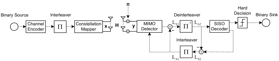
Figure 2: BICM transmitter and IDD receiver in an MIMO system.

Based on Klein’s sampling algorithm [17], the probability of $F(\widetilde{x}_{i})$ returning an integer $\widehat{x}_{i}^{j}$ ($1\leq j\leq 2N$) from the 2$N$-integer set is calculated from the following discrete Gaussian distribution

$$\begin{split}P(\widehat{x}^{j}_{i})&=\frac{e^{-c_{i}(\widetilde{x}_{i}-\widehat{x}^{j}_{i})^{2}}}{s},\end{split}$$ (7)

where

$$\begin{split}s=s(c_{i})&=\sum_{\widehat{x}^{l}_{i}\in\mathcal{I}}e^{-c_{i}(\widetilde{x}_{i}-\widehat{x}^{l}_{i})^{2}}\end{split}$$ (8)

and $c_{i}=Ar^{2}_{i,i}$. Note that $P(\widehat{x}^{j}_{i})$ is a conditional probability because the selection of previous entries are also taken into account to calculate $\widetilde{x}_{i}$. As for the selection of the parameter $A$ which affects the variance of sampling probabilities, Klein chose $A=\text{log}n/\text{min}_{i}r_{i,i}^{2}$ and [16] gave a better parameter for randomized sampling algorithm as $A=\text{log}\rho/\text{min}_{i}r_{i,i}^{2}$ where the parameter $\rho>1$ related with the sample size $K$ follows

$$K=(e\rho)^{2n/\rho}.$$ (9)

The decisions $\widehat{x}_{i}$’s are generated level by level, and a candidate lattice point $\widehat{\mathbf{x}}$ is obtained if all the entries are generated. It has been demonstrated in [16] that given ${\mathbf{y}}$, the probability of a vector $\mathbf{\hat{x}}$ being sampled (also known as the sampling probability of $\mathbf{\hat{x}}$) is lower bounded by

$$P(\mathbf{\hat{x}})\geq\frac{1}{\prod^{n}_{i=1}s(Ar_{i,i}^{2})}e^{-A\|{\mathbf{y}}-\mathbf{H\hat{x}}\|^{2}}.$$ (10)

By repeating this sampling procedure for $K$ times, a candidate list of $K$ lattice points is obtained as shown in Fig. 1 and the closest one in Euclidean norm is chosen as the decoding output.

However, because samplings are random and because the $K$ samples are independent of each other, lattice points are sampled following the probability $P=1-(1-P(\mathbf{x}))^{K}$, which results in two inherent problems in random sampling. On one hand, inevitable sample repetitions in the final candidate list means unnecessary complexity is incurred. Meanwhile, the performance is also degraded by the existence of repetitions since most of samplings are employed to sample those lattice points with large sampling probabilities. On the other hand, lattice points have to face the risk of being missed during the sampling, especially for those with small sampling probabilities on the early decoding levels, leading to inevitable performance loss. Actually, to make sure lattice points with a reasonable probability to be sampled, one has to increase the sample size $K$, which leads to more sampling repetitions. Therefore, the efficiency and performance of the randomized sampling are greatly suffered from the randomization.

II-B Soft-Output Decoding

In order to achieve near-capacity performance with low complexity in MIMO-BICM systems, iterative detection and decoding (IDD) proposed in [9] has attracted much attention recently, which improves the performance by iteratively exchanging the extrinsic information between MIMO detector and soft-in soft-out (SISO) decoder.

As shown in Fig. 2, the extrinsic information $L_{E1}$ is calculated by the MIMO detector based on the channel observation $\mathbf{y}$ and a priori information (API) $L_{A1}$ of the transmitted bits which is provided by the SISO decoder. Then $L_{E1}$ is passed through the deinterleaver to become API $L_{A2}$ to the SISO decoder, which computes the new extrinsic information $L_{E2}$ to feed back to the MIMO detector. Specifically, the extrinsic information in soft-output decoding is always calculated through the computation of the posterior LLR for each information bit associated with the transmitted signal $\mathbf{x}$, which is given as

$$L(b_{i}|\mathbf{y})=\text{log}\frac{P(b_{i}=1|\mathbf{y})}{P(b_{i}=0|\mathbf{y})}$$ (11)

where $b_{i}$ is the $i$-th information bit in $\mathbf{x}$, $1\leq i\leq mn$. Here, $m$ represents the number of bits per constellation symbol and $\mathbf{x}$ contains $mn$ information bits in all. Through the exchange of extrinsic information in each iteration, the performance of soft-output decoding improves gradually and we have

$$L(b_{i}|\mathbf{y})\ \ \ \ \ \ \ \ \ \ \ \ \ \ \ \ \ \ \ \ \ \ \ \ \ \ \ \ \ \ \ \ \ \ \ \ \ \ \ \ \ \ \ \ \ \ \ \ \ \ \ \ \ \ \ \$$

$$=L_{\textrm{A}}(b_{i})+\text{log}\frac{\sum_{\mathbf{x}:b_{i}=1}P(\mathbf{y}|\mathbf{x})\cdot\text{exp}\sum_{j\in\mathcal{J}_{i}}L_{\textrm{A}}(b_{j})}{\sum_{\mathbf{x}:b_{i}=0}P(\mathbf{y}|\mathbf{x})\cdot\text{exp}\sum_{j\in\mathcal{J}_{i}}L_{\textrm{A}}(b_{j})}$$ (12)

where $L_{\textrm{A}}(b_{i})$ denotes API of each transmitted bit in $\mathbf{x}$

$$L_{\textrm{A}}(b_{i})=\text{log}\frac{P(b_{i}=1)}{P(b_{i}=0)}$$ (13)

and $\mathcal{J}_{i}$ is the set of indices $j$ with

$$\mathcal{J}_{i}=\{j|j=1,\ldots,mn,j\neq i\}.$$ (14)

In the absence of API, we suppose all the bits in $\mathbf{x}$ have the same probability to be 0 or 1 before $\mathbf{y}$ is observed as $P(b_{i}=1)=P(b_{i}=0)=\frac{1}{2}$. Then, for simplicity, the $L$-value in (11) becomes [9, 18]

$$L(b_{i}|\mathbf{y})=\text{log}\frac{\sum_{\mathbf{x}:b_{i}=1}\text{exp}\ (-\frac{1}{2\sigma^{2}}\parallel\mathbf{y}-\mathbf{H}\mathbf{x}\parallel^{2})}{\sum_{\mathbf{x}:b_{i}=0}\text{exp}\ (-\frac{1}{2\sigma^{2}}\parallel\mathbf{y}-\mathbf{H}\mathbf{x}\parallel^{2})}.$$ (15)

The straightforward way to calculate the $L$-value in (15) is MAP algorithm which computes the sums that contain $2^{mn}$ terms. Due to the exponentially increased complexity of MAP, one has to resort to approximations to reduce the complexity.

As one of the approximation scenarios, Max-Log approximation tries to approximate the sums in (15) only with their largest terms [19, 20]:

$$L(b_{i}|\mathbf{y})\approx\text{log}\frac{\text{max}_{\mathbf{x}:b_{i}=1}\text{exp}\ (-\frac{1}{2\sigma^{2}}\parallel\mathbf{y}-\mathbf{H}\mathbf{x}\parallel^{2})}{\text{max}_{\mathbf{x}:b_{i}=0}\text{exp}\ (-\frac{1}{2\sigma^{2}}\parallel\mathbf{y}-\mathbf{H}\mathbf{x}\parallel^{2})}.$$ (16)

However, to obtain the largest terms in (16), sphere decoding is applied, which incurs exponential increment complexity. To achieve a polynomial complexity, suboptimal hard decoding schemes like SIC are used to solve those maximization problems approximately. Unfortunately, the decoder performance is poor even under the help of the lattice reduction technique.

As for another approximation schemes, list sphere decoding (LSD) proposed in [9] restricts the sums in (15) into a much smaller size, which uses sphere decoding with a certain radius to perform the candidate admission as follows

$$\mathcal{S}\triangleq\{\mathbf{x}\in\mathcal{X}^{n}:\|\mathbf{y}-\mathbf{Hx}\|^{2}\leq R^{2}\}.$$ (17)

Here, $R$ denotes the sphere radius and a larger $R$ means a better approximation and also, a higher computational complexity. Then, the calculation of L-value in (15) can be written as

$$L(b_{i}|\mathbf{y})\approx\text{log}\frac{\sum_{\mathbf{x}\in\mathcal{S}:b_{i}=1}\text{exp}\ (-\frac{1}{2\sigma^{2}}\parallel\mathbf{y}-\mathbf{H}\mathbf{x}\parallel^{2})}{\sum_{\mathbf{x}\in\mathcal{S}:b_{i}=0}\text{exp}\ (-\frac{1}{2\sigma^{2}}\parallel\mathbf{y}-\mathbf{H}\mathbf{x}\parallel^{2})}.$$ (18)

Although lattice reduction technique can be applied to reduce its complexity, LSD schemes still suffer from a high complexity cost due to the application of sphere decoding. In particular, unlike finding the closest lattice point in lattice decoding, sphere decoding in LSD tries to enumerate all the lattice points within a constant sphere radius $R$. Additionally, since the selection of the sphere radius $R$ affects the performance of LSD, there is still an open question about the upper bound of $R$ when LSD achieves near-MAP performance.

III Derandomized Sampling Decoding

In this section, we propose a derandomized sampling algorithm to solve the afore-mentioned problems in randomized sampling decoding, namely, repetition and missing of certain lattice points. Specifically, the sampling procedure of the derandomized sampling algorithm is performed level by level with $i=n,n-1,\ldots,1$ as follows:

Algorithm 1 Derandomized sampling on decoding level $i$

Compute $\widetilde{x}_{i}=\frac{y^{\prime}_{i}-\sum^{n}_{l=i+1}r_{i,l}\widehat{x}_{l}}{r_{i,i}}$

for $j=$1,2,…,2$N$ do

     Compute $P(\widehat{x}^{j}_{i})=\frac{e^{-c_{i}(\widetilde{x}_{i}-\widehat{x}^{j}_{i})^{2}}}{s}$

     Compute $E(\widehat{x}^{j}_{i})=\lceil K_{i+1}P(\widehat{x}^{j}_{i})\rfloor$

     if $E(\widehat{x}^{j}_{i})<1$ then

         $\widehat{x}^{j}_{i}$ is ignored, sampling based on $\widehat{x}^{j}_{i}$ terminates

     else if $E(\widehat{x}^{j}_{i})=1$ then

         Let $\widehat{x}_{i}=\widehat{x}^{j}_{i}$, SIC is performed based on the detected

         entries $\widehat{x}_{n},\ldots,\widehat{x}_{i}$ to return a candidate lattice point

     else if $E(\widehat{x}^{j}_{i})>1$ then

         if $i>1$ then

              Let $\widehat{x}_{i}=\widehat{x}^{j}_{i}$, $K_{i}=K_{i+1}P(\widehat{x}^{j}_{i})$, start derandomi-

              zed sampling from the next level $i-1$ based on

              the detected entries $\widehat{x}_{n},\ldots,\widehat{x}_{i}$

         else if $i=1$ then

              Let $\widehat{x}_{1}=\widehat{x}^{j}_{1}$, return $\widehat{x}_{n},\ldots,\widehat{x}_{1}$ as a candidate

              lattice point

         end if

     end if

end for

At decoding level $i$, sample size $K_{i+1}$ is allocated to candidate integers according to $K_{i}=K_{i+1}P(\widehat{x}^{j}_{i})$ and all the integers with $E(\widehat{x}^{j}_{i})\geq 1$ are deterministically sampled. Note that $K_{i}$ is not necessarily an integer any more. For integers with $E(\widehat{x}^{j}_{i})>1$, after updating the size $K_{i}$, sampling continues from the next level in the same way. Note that when $K=1$, derandomized sampling decoding performs the same with SIC decoding by always selecting the integer with the largest probability. Hence, for integers with $E(\widehat{x}^{j}_{i})=1$, SIC is applied directly to obtain a candidate lattice point. Finally, among all the candidate lattice points, the closest one is selected as the solution. By performing the sampling based on the threshold $E(\widehat{x}^{j}_{i})\geq 1$ at each decoding level, the whole sampling process becomes deterministic. The risk of lattice points being missed during the sampling is greatly reduced, which means the probability of sampling the closest lattice point is improved.

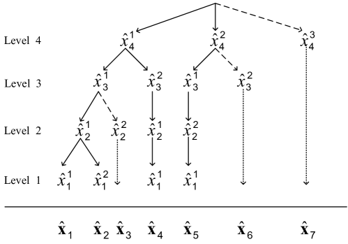
Figure 3: Illustration of the tree structure in derandomized sampling decoding with ${n}=4$. The solid and dashed lines represent the corresponding candidate integer being sampled by $E(\widehat{x}^{j}_{i})>1$ and $E(\widehat{x}^{j}_{i})=1$ respectively. The dotted line denotes performing SIC detection in the rest of levels due to $E(\widehat{x}^{j}_{i})=1$.

Unlike the parallel structure of the random sampling, derandomized sampling decoding admits a tree structure as shown in Fig. 3. The final candidate list is generated by traversing the tree from level $n$ to level 1 rather than by $K$ independent paths. From this perspective, derandomized sampling functions like a pruning algorithm in sphere decoding [21, 22, 23] which prunes branches $E(\widehat{x}^{j}_{i})<1$. Thanks to the tree structure, there are no sampling repetitions during the whole sampling process while necessary calculations of sampling probabilities $P(\widehat{x}^{j}_{i})$ in branches $E(\widehat{x}^{j}_{i})>1$ are performed only once, saving a lot of complexity. Therefore, different from randomized sampling decoding and other decoding schemes establishing a candidate list with a constant size around the SIC output [12, 24], the size of the final candidate list $K_{\text{final}}\leq K$ is variable, which means the sample size $K$ set initially in the derandomized sampling algorithm is actually a nominal sample size of the candidate list.

As a nominal sample size, $K$ is essentially a parameter in the threshold $E(\widehat{x}^{j}_{i})=\lceil K_{i+1}P(\widehat{x}^{j}_{i})\rfloor\geq 1$ used to evaluate the sampling performance. With the increment of $K$, the complexity improves gradually since more lattice points will be sampled. Note that $K$ is not the real size of the final sampling list, the complexity of derandomized sampling decoding in fact grows slowly with its increment. Because problems caused by randomization are overcome, derandomized algorithm achieves desirable improvement in both performance and complexity.

III-A Algorithm Analysis

The operation of the derandomized sampling algorithm relies on the notion of the sampling probability which is calculated by (7). According to the defined threshold $E(\widehat{x}^{j}_{i})\geq 1$, at each decoding level, an integer candidate $\widehat{x}_{i}^{j}$ for the entry $x_{i}$ will be sampled if and only if

$$K_{i+1}P(\widehat{x}_{i}^{j})\geq\frac{1}{2}.$$ (19)

Note that the sampling probability $P(\widehat{x}_{i}^{j})$ calculated by (7) is a conditional probability based on the entries of previous levels. As sampling is performed from level $n$ to level 1, the sampling probability $P(\mathbf{x})$ about lattice point $\mathbf{x}$ is essentially the product of its entries’ sampling probability, which is lower bounded by (10):

$$P(\mathbf{x})=\prod_{i=1}^{n}P(\widehat{x}_{n+1-i}^{j})\geq\frac{1}{\prod^{n}_{i=1}s(Ar_{i,i}^{2})}e^{-A\|{\mathbf{y}}-\mathbf{Hx}\|^{2}}.$$ (20)

Proposition 1.

Given the nominal sample size $K$, lattice points with sampling probability

$$P(\mathbf{x})\geq\frac{1}{2K}$$ (21)

will be deterministically sampled by derandomized sampling algorithm.

Proof: Consider sampling an $n$-dimensional lattice point $\mathbf{x}$ by derandomized sampling algorithm. Obviously, with the initial sample size $K$, its first entry $\widehat{x}_{n}^{j}$ on level $n$ will be sampled if

$$KP(\widehat{x}_{n}^{j})\geq\frac{1}{2}.$$ (22)

Based on the selection of $\widehat{x}_{n}^{j}$, its updated sample size $K_{n}$ on the next level is calculated as

$$K_{n}=KP(\widehat{x}_{n}^{j}).$$ (23)

Then, on level $n-1$, the first two entries of $\mathbf{x}$ will be obtained when

$$K_{n}P(\widehat{x}_{n-1}^{j})=KP(\widehat{x}_{n}^{j})P(\widehat{x}_{n-1}^{j})\geq\frac{1}{2}.$$ (24)

By induction, $\mathbf{x}$ will be deterministically sampled if the following condition holds

$$K\prod_{i=1}^{n}P(\widehat{x}_{n+1-i}^{j})=KP(\mathbf{x})\geq\frac{1}{2}.$$ (25)

Thus, the conclusion follows, completing the proof.

As for the randomized sampling in [16], because the $K$ times sampling is independent of each other, the probability of missing $\mathbf{x}$ is calculated as $(1-P(\mathbf{x}))^{K}$, which means one has to increase the sample size $K$ to ensure $\mathbf{x}$ a high probability of being sampled. In particular, given sample size $K$, lattice points with sampling probability

$$P(\mathbf{x})\geq\frac{1}{K}$$ (26)

will be found by randomized sampling algorithm with probability $P\geq 1-1/e$. Through the comparison between (21) and (26), to sample the same lattice point $\mathbf{x}$, the required sample size of the derandomized sampling algorithm is less than the half of that in randomized sampling algorithm:

$$K_{\text{Derandomized}}<\frac{1}{2}K_{\text{Random}}.$$ (27)

On the other hand, with the same sample size $K_{\text{Derandomized}}=K_{\text{Random}}$, derandomized sampling algorithm has the ability to obtain more lattice points than randomized sampling, which brings further performance improvement. Since $K_{\text{Derandomized}}$ is the nominal sample size, for the same sample size derandomized sampling algorithm still achieves much lower complexity than randomized sampling. More precisely, when $K=1$, the complexity of the derandomized sampling algorithm is $O(n^{2})$ by invoking the calculation of the sampling probability in (7) for $n$ times. For $K>1$, as computations in sampling procedures are reduced by removing all the repetitions, the number of recalling the calculation in (7) is much less than $Kn$, which means the complexity is much smaller than $K\cdot O(n^{2})$. Due to the uncertainty in this procedure, it is preferable to denote the complexity of the derandomized sampling algorithm by $K\cdot O(n^{2})$, which means a polynomial complexity with respect to the dimension $n$. Obviously, without suffering from the effect of the randomization, derandomized sampling algorithm shows great potential in both performance and complexity.

III-B Optimization of the Parameter $A$

As a parameter which controls the variance of sampling probabilities, parameter $A$ has a significant impact on the final decoding performance. Due to the consideration of complexity, the initial sample size $K$ of sampling algorithms is always limited, which means finding the optimum $A$ to exploit the sampling potential for a given $K$ is the key. In order to determine the optimum choice of $A$ in the derandomized sampling algorithm, let $A=\text{log}\rho/\text{min}_{i}r_{i,i}^{2}$ where $\rho>1$, then $\rho$ becomes the parameter needed to be optimized.

It has been demonstrated in [17] that

$$\overset{n}{\underset{i=1}{\prod}}s(c_{i})\leq e^{\frac{2n}{\rho}(1+O(\rho^{-3}))}.$$ (28)

Because $\rho>1$, the term $O(\rho^{-3})$ in (28) will be negligible if $\rho$ is sufficiently large. Assume $\rho$ satisfies this weak condition, the sampling probability of $\mathbf{x}$ shown in (20), which is calculated based on the discrete Gaussian distribution, can be further derived as follows

$$P(\mathbf{x})\geq e^{-\frac{2n}{\rho}}\cdot\rho^{-\|\mathbf{y}-\mathbf{H}\mathbf{x}\|^{2}/\text{min}_{i}r_{i,i}^{2}}.$$ (29)

Since lattice points with $P(\mathbf{x})\geq\frac{1}{2K}$ will be deterministically sampled by derandomized sampling algorithm, motivated by (29), let

$$e^{-\frac{2n}{\rho}}\cdot\rho^{-\|\mathbf{y}-\mathbf{H}\mathbf{x}\|^{2}/\text{min}_{i}r_{i,i}^{2}}\geq\frac{1}{2K},$$ (30)

and we have

$$\|\mathbf{y}-\mathbf{H}\mathbf{x}\|\leq\text{min}_{i}r_{i,i}\cdot\sqrt{\text{log}_{\rho}(2Ke^{-2n/\rho})},$$ (31)

which means lattice points with $\|\mathbf{y}-\mathbf{H}\mathbf{x}\|$ less than the right-hand side (RHS) of (31) must be obtained.

In order to exploit the potential of the derandomized sampling algorithm for the best decoding performance, parameter $\rho$ is selected carefully to maximize the upper bound shown in (31). Therefore, let the derivative about $\text{log}_{\rho}(2Ke^{-2n/\rho})$ versus $\rho$ be zero, the optimum $\rho_{\text{o}}$ given sample size $K$ in the derandomized sampling algorithm can be finally determined as follows

$$K=\frac{1}{2}(e\rho_{\text{o}})^{2n/\rho_{\text{o}}}.$$ (32)

Obviously, the optimum $\rho_{\text{o}}$ for the randomized sampling algorithm shown in (9) is not the optimum solution in the derandomized sampling algorithm. According to (32), it is easy to check that the parameter $\rho_{\text{o}}$ monotonically decreases with respect to the increment of the sample size $K$.

In the view of lattice decoding, derandomized sampling algorithm will give the closest lattice point if the distance between $\mathbf{y}$ and lattice $\mathcal{L}(\mathbf{H})$ is less than the RHS of (31). Therefore, the RHS of (31) can be regarded as the decoding radius in the notion of bounded distance decoding (BDD). By substituting (32) into (31), the optimum decoding radius $R_{\text{Derandomized}}$ of the derandomized sampling algorithm is derived as

$$R_{\text{Derandomized}}\triangleq\sqrt{\frac{2n}{\rho_{\text{o}}}}\ \text{min}_{i}r_{i,i}.$$ (33)

Clearly, with the increment of $K$, $R_{\text{Derandomized}}$ improves gradually resulting in better decoding performance. We need to emphasize that the decoding radius $R_{\text{Derandomized}}$ may be much larger than the value defined in (33) because the derivation is only based on the lower bound of $P(\mathbf{x})$ shown in (29).

III-C Upper Bound on the Sample Size $K$

We now give an explicit value of $K$ when derandomized sampling decoding achieves near-ML performance. To do this, the total probability of samples in the final candidate list is derived based on the truncation of the discrete Gaussian distribution (7).

As shown in [16], the probability that the integer $\widehat{x}_{i}$ generated by random rounding $F(\widetilde{x}_{i})$ is located within the 2N integers around $\widetilde{x}_{i}$ is bounded by

$$P_{2N}\geq 1-O(\rho^{-N^{2}}).$$ (34)

Because $\rho>1$, the term $O(\rho^{-N^{2}})$ decays exponentially, meaning a finite truncation with moderate $N$ achieves an accurate approximation. Normally, 3-integer approximation is sufficient:

$$P(\widehat{x}_{i}^{1})+P(\widehat{x}_{i}^{2})+P(\widehat{x}_{i}^{3})\approx 1.$$ (35)

Since these probabilities follow the discrete Gaussian distribution, they decrease monotonically with the distance from $\widetilde{x}_{i}$. Let us order them as follows

$$P(\widehat{x}_{i}^{1})\geq P(\widehat{x}_{i}^{2})\geq P(\widehat{x}_{i}^{3}).$$ (36)

As shown in (4), $\widetilde{x}_{i}$ is subject to the effect of noise. Intuitively, $\widetilde{x}_{i}$ tends to be close to an integer for small noise while it tends to be halfway between two integers for large noise. Since $\widetilde{x}_{i}$ is the peak of the continuous Gaussian distribution associated with the discrete one (7), we define the worst case in sampling as the one where $\widetilde{x}_{i}$ is centered between two integers.

Because the random noise makes it hard for an exact analysis, we only consider the worst-case scenario in samplings. Then, under the 3-integer approximation in (35), the following holds in the worst case:

$$P(\widehat{x}_{i}^{1})=P(\widehat{x}_{i}^{2})\gg P(\widehat{x}_{i}^{3})$$ (37)

where $P(\widehat{x}_{i}^{3})$ is much smaller due to exponential decay of the probability with the distance.

Now, let us calculate the total probability of lattice points sampled by derandomized sampling, in the worst case. Consider the level $n$ first. Obviously, according to (19), the first two integers will be sampled if $K>2$. If $P(\widehat{x}^{3}_{n})\geq\frac{1}{2K}$, all the 3 integers around $\widetilde{x}_{n}$ are deterministically sampled. On the other hand, if $P(\widehat{x}^{3}_{n})<\frac{1}{2K}$, integer $\widehat{x}^{3}_{n}$ will be discarded while the summation of probabilities of the other two integers will be larger than $1-\frac{1}{2K}$ according to (35). Therefore, given the nominal sample size $K$, the sum probability of samples on the level $n$ is bounded by

$$P(\text{level}\,n)\geq 1-\frac{1}{2K}.$$ (38)

To further derive the lower bound of the total probability of samples, we assume the third sample $\widehat{x}^{3}_{i}$ at the each sampling level is always discarded. Then, still in the worst case, the total probability of samples on the level $n-1$ is given by

$$P(\text{level}\,n-1)\geq(1-\frac{1}{2K})\left[\frac{1}{2}\left(1-\frac{1}{K}\right)+\frac{1}{2}\left(1-\frac{1}{K}\right)\right]$$

$$\,\,\,\,\,\,\,\,\,\,\,\,\,\,\,\,\,\,\,\,\,\,\,\,\,\,\,\,\,\,\,\,\,\,\,\,=(1-\frac{1}{2K})(1-\frac{1}{K}).$$ (39)

Similarly, on the level $n-p$, the total probability of samples in the worst case can be lower bounded by

$$P(\text{level}\,n-p)>\prod_{i=1}^{p}(1-\frac{2^{i-2}}{K}).$$ (40)

Therefore, the total probability of sampled lattice points in the derandomized sampling algorithm is lower bounded by a function of $K$. We define a parameter $\eta$ to evaluate the decoding performance as

$$P_{\textrm{total}}=P(\text{level}\,1)>\eta\triangleq\prod_{i=1}^{n}(1-\frac{2^{i-2}}{K}).$$ (41)

Obviously, the lower bound $\eta$ increases with $K$ and a larger $\eta$ means a higher probability of the closest lattice point being sampled. Thus, derandomized sampling decoding can be used to approximate ML decoding as $\eta$ approaches 1.

The lower bound (41) is loose because it quantifies the probability in the worst case. For $\eta$ close to 1, $K$ can be very huge (in fact exponential). A lower bound in the average case is an open question. Because the noise is random, the average-case probability may be more useful.

In order to obtain a better estimate, the idea of the fixed-complexity sphere decoding (FSD), which also follows a tree structure in decoding, is exploited. Different from the standard sphere decoding, it only performs the full search in the upper $p$ levels known as the full-expansion stage while SIC is applied on the rest of levels. It has been proved in [25] that by applying the channel matrix ordering to make sure signals with the largest postprocessing noise amplification are detected in the full-expansion stage, FSD algorithm yields near-ML performance in high SNR if it satisfies:

$$(p+1)^{2}\geq n$$ (42)

where $p$ is the number of levels in the full-expansion stage.

We propose to use sampling in the full-expansion stage of FSD. With the suitable channel matrix ordering, the modified sampling decoder also consists of two stages. Candidate values on the upper $p$ levels are sampled based on the lower bound $\eta$ while decodings on the remaining levels are processed by SIC (i.e., derandomized sampling decoding with $K=1$).

According to (40) and (42), if we set $\eta$ to a value near 1 on the upper $p$ decoding levels, then the decoder will achieve near-ML performance:

$$P_{\textrm{total}}=P(\text{level}\,n-p)>\eta=\prod_{i=1}^{p}(1-\frac{2^{i-2}}{K}).$$ (43)

Compared with (41), the lower bound (43) is better because $p$ is much smaller than $n$ meaning the value of $K$ achieving the same $\eta$ is greatly reduced. Here, we define $\eta=0.9$ representing near-ML performance. Then, according to (43), the corresponding $K$ who denotes the upper bound of the sample size in derandomized sampling decoding can be easily calculated.

Note that the derandomized sampling algorithm with $K=1$ performs the same with SIC in lattice decoding. Thus, the decoder enjoys flexible performance between SIC and near-ML by adjusting $K$. Although larger $\eta>0.9$ will bring further performance improvement, it approaches ML performance asymptotically with the exponential increment of $K$, which is meaningless due to the consideration of complexity.

IV Derandomized sampling algorithm in soft-output decoding

In this section, we show that the proposed derandomized sampling algorithm can also be used as an efficient tool to implement soft-output decoding in MIMO systems. By generating a list of lattice points around the ML estimate $\text{min}_{\mathbf{x}\in\mathcal{X}^{n}}\|\mathbf{y}-\mathbf{Hx}\|$, derandomized sampling algorithm in soft-output decoding actually functions as an approximation scheme like list sphere decoding (LSD) in [9]. To establish the trade-off with respect to the sample size $K$, we firstly give an upper bound of the sphere radius $R$ in LSD.

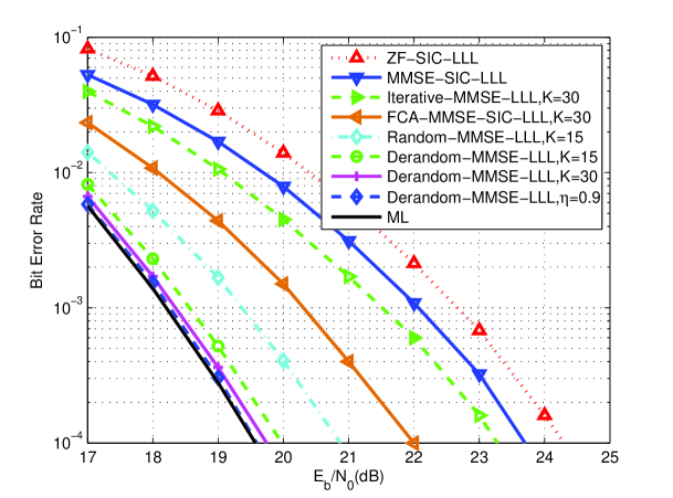
Figure 4: Bit error rate versus average SNR per bit for the uncoded $10\times 10$ MIMO system using 64-QAM.

IV-A Upper Bound on the Sphere Radius $R$ in LSD

Given $\mathbf{y}\in\mathbb{R}^{n}$, we define a function $f:\mathbb{R}^{n}\rightarrow\mathbb{R}$ over the $n$-dimensional lattice $\mathcal{L}(\mathbf{H})$ as

$$f_{\mathcal{L}(\mathbf{H})}(\mathbf{y})=\frac{\sum_{\mathbf{v}\in\mathcal{L}(\mathbf{H})}\text{exp}(-\pi\|\mathbf{y}-\mathbf{v}\|^{2})}{\sum_{\mathbf{v}\in\mathcal{L}(\mathbf{H})}\text{exp}(-\pi\|\mathbf{v}\|^{2})},$$ (44)

where $\mathbf{v}\in\mathbb{R}^{n}$ denotes the lattice point of $\mathcal{L}(\mathbf{H})$. Thus the LLR in soft-output decoding shown in (15) can be expressed by $f$-function as

$$L(b_{i}\mid\mathbf{y}) = \text{log}\frac{\sum_{\mathbf{x}:b_{i}=1}\text{exp}(-\pi\cdot\frac{1}{2\pi\sigma^{2}}\parallel\mathbf{y}-\mathbf{H}\mathbf{x}\parallel^{2})}{\sum_{\mathbf{x}:b_{i}=0}\text{exp}(-\pi\cdot\frac{1}{2\pi\sigma^{2}}\parallel\mathbf{y}-\mathbf{H}\mathbf{x}\parallel^{2})}$$ (45)

$$= \text{log}\frac{\frac{\sum_{\mathbf{x}:b_{i}=1}\text{exp}(-\pi\cdot\frac{1}{2\pi\sigma^{2}}\parallel\mathbf{y}-\mathbf{H}\mathbf{x}\parallel^{2})}{\sum_{\mathbf{x}\in\mathcal{X}^{n}}\text{exp}(-\pi\cdot\frac{1}{2\pi\sigma^{2}}\parallel\mathbf{H}\mathbf{x}\parallel^{2})}}{\frac{\sum_{\mathbf{x}:b_{i}=0}\text{exp}(-\pi\cdot\frac{1}{2\pi\sigma^{2}}\parallel\mathbf{y}-\mathbf{H}\mathbf{x}\parallel^{2})}{\sum_{\mathbf{x}\in\mathcal{X}^{n}}\text{exp}(-\pi\cdot\frac{1}{2\pi\sigma^{2}}\parallel\mathbf{H}\mathbf{x}\parallel^{2})}}$$

$$= \text{log}\frac{f_{\mathcal{L}(\frac{1}{\sigma\sqrt{2\pi}}\mathbf{H}),\mathbf{x}:b_{i}=1}(\frac{1}{\sigma\sqrt{2\pi}}\mathbf{y})}{f_{\mathcal{L}(\frac{1}{\sigma\sqrt{2\pi}}\mathbf{H}),\mathbf{x}:b_{i}=0}(\frac{1}{\sigma\sqrt{2\pi}}\mathbf{y})}.$$

Accordingly, the $L$-value computation is converted into the calculation of function $f_{\mathcal{L}(\frac{1}{\sigma\sqrt{2\pi}}\mathbf{H})}(\frac{1}{\sigma\sqrt{2\pi}}\mathbf{y})$. Here, the lattice point $\mathbf{v}$ in $\mathcal{L}(\mathbf{H})$ is expressed by $\mathbf{Hx}$, where $\mathbf{x}\in\mathcal{X}^{n}$ is an integer vector. To further exploit the function $f$, we invoke the following lemma in [26].

Lemma 1 ([26]). For any n-dimensional lattice $\mathcal{L}(\mathbf{H})$, $\mathbf{y}\in\mathbb{R}^{n}$ and $c>\frac{1}{\sqrt{2\pi}}$, one has

$$\frac{\sum_{\mathbf{v}\in\mathcal{L}(\mathbf{H}),\parallel\mathbf{y}-\mathbf{v}\parallel>c\sqrt{n}}\text{exp}(-\pi\|\mathbf{y}-\mathbf{v}\|^{2})}{\sum_{\mathbf{v}\in\mathcal{L}(\mathbf{H})}\text{exp}(-\pi\|\mathbf{v}\|^{2})} \leq 2\left(c\sqrt{2\pi e}\cdot e^{-\pi c^{2}}\right)^{n}$$ (46)

$$= 2^{-\Omega(n)}.$$

According to Lemma 1, we obtain

$$f_{\mathcal{L}(\mathbf{H})}(\mathbf{y})=\frac{\sum_{\mathbf{v}\in\mathcal{L}(\mathbf{H}),\|\mathbf{y}-\mathbf{v}\|\leq c\sqrt{n}}\text{exp}(-\pi\|\mathbf{y}-\mathbf{v}\|^{2})}{\sum_{\mathbf{v}\in\mathcal{L}(\mathbf{H})}\text{exp}(-\pi\|\mathbf{v}\|^{2})}\ \ \ \ \ \ \ \ \ \ \ \ \ \ \ \ \ \$$

$$+\frac{\sum_{\mathbf{v}\in\mathcal{L}(\mathbf{H}),\|\mathbf{y}-\mathbf{v}\|>c\sqrt{n}}\text{exp}(-\pi\|\mathbf{y}-\mathbf{v}\|^{2})}{\sum_{\mathbf{v}\in\mathcal{L}(\mathbf{H})}\text{exp}(-\pi\|\mathbf{v}\|^{2})}\ \ \ \ \ \ \ \ \ \ \$$

$$\ \ \ \leq\frac{\sum_{\mathbf{v}\in\mathcal{L}(\mathbf{H}),\|\mathbf{y}-\mathbf{v}\|\leq c\sqrt{n}}\text{exp}(-\pi\|\mathbf{y}-\mathbf{v}\|^{2})}{\sum_{\mathbf{v}\in\mathcal{L}(\mathbf{H})}\text{exp}(-\pi\|\mathbf{v}\|^{2})}+2^{-\Omega(n)}.$$ (47)

As to the second term in the RHS of (47), it decays exponentially with the dimension $n$. Assume $n$ is sufficiently large, then $f_{\mathcal{L}(\mathbf{H})}(\mathbf{y})$ is dominated by the set of lattice points within the radius $R=\sqrt{n/2\pi}$ centering at $\mathbf{y}$. Back to $f_{\mathcal{L}(\frac{1}{\sigma\sqrt{2\pi}}\mathbf{H})}(\frac{1}{\sigma\sqrt{2\pi}}\mathbf{y})$ in (45), correspondingly, lattice points in the corresponding set denoted by $S$ should satisfy the following condition as

$$\frac{1}{\sigma\sqrt{2\pi}}\|\mathbf{y}-\mathbf{v}\| \leq \sqrt{\frac{n}{2\pi}}$$ (48)

and we have

$$\|\mathbf{y}-\mathbf{v}\| \leq \sqrt{n}\sigma.$$ (49)

Based on the fact as shown in (45) that

$$f_{\mathcal{L}(\frac{1}{\sigma\sqrt{2\pi}}\mathbf{H})}(\frac{1}{\sigma\sqrt{2\pi}}\mathbf{y})\propto\sum_{\mathbf{x}\in\mathcal{X}^{n}}\text{exp}\ (-\frac{1}{2\sigma^{2}}\parallel\mathbf{y}-\mathbf{H}\mathbf{x}\parallel^{2}),$$ (50)

the key of solving the $L$-value computation depends on lattice points within the radius $\sqrt{n}\sigma$. In other words, it can be interpreted as that, with the sphere radius $R=\sqrt{n}\sigma$, LSD could achieve MAP performance within a negligible loss by only exploiting lattice points in the set $S$ shown in (17). Thus, the sphere radius $R$ in LSD is upper bounded by

$$R\leq\sqrt{n}\sigma.$$ (51)

Note that with the increase of SNR, the radius $R$ shrinks gradually saving a lot of complexity.

IV-B Derandomized Sampling in Soft-Output Decoding

Given the sphere radius $R$, LSD performs sphere decoding to obtain all the lattice points within $R$. However, it is known that sphere decoding is impractical due to its exponentially increased complexity. Instead of enumerating lattice points within $R$ by exhaustive search, derandomized sampling algorithm generates lattice points by sampling from a Gaussian-like distribution, which is more efficient than LSD due to its polynomial complexity.

As it shown in (10), the lower bound of the sampling probability resembles a Gaussian distribution over the lattice. The closer $\mathbf{Hx}$ to $\mathbf{y}$, the larger lower bound. Therefore, lattice points closer to $\mathbf{y}$ are more likely to be sampled due to larger sampling probability lower bounds. In this way, the derandomized sampling algorithm could find a number of lattice points with small values of $\|\mathbf{y}-\mathbf{Hx}\|$ around the ML estimate. By restricting the original set of sums in (15) into a much smaller one denoted by $\mathcal{C}$, the LLR calculation by derandomized sampling algorithm can be written as

$$L(b_{i}|\mathbf{y})\approx\text{log}\frac{\sum_{\mathbf{x}\in\mathcal{C}:b_{i}=1}\text{exp}\ (-\frac{1}{2\sigma^{2}}\parallel\mathbf{y}-\mathbf{H}\mathbf{x}\parallel^{2})}{\sum_{\mathbf{x}\in\mathcal{C}:b_{i}=0}\text{exp}\ (-\frac{1}{2\sigma^{2}}\parallel\mathbf{y}-\mathbf{H}\mathbf{x}\parallel^{2})}.$$ (52)

It is noteworthy that lattice points with sampling probabilities $P(\mathbf{x})\geq\frac{1}{2K}$ will be deterministically sampled by derandomized sampling algorithm. As shown in (31), this can be interpreted as obtaining all the lattice points inside a sphere of the radius $r$ where

$$r=\|\mathbf{y}-\mathbf{H}\mathbf{x}\|\leq\text{min}_{i}r_{i,i}\cdot\sqrt{\text{log}_{\rho}(2Ke^{-2n/\rho})}.$$ (53)

To achieve a better upper bound of $r$, the optimum choice of the parameter $\rho_{o}$ in (32) is applied and we have

$$r\leq\sqrt{\frac{2n}{\rho_{\text{o}}}}\ \text{min}_{i}r_{i,i}.$$ (54)

Let $\mathcal{C}_{1}$ denotes the set formed by lattice points within sphere radius $r$

$$\mathcal{C}_{1}\triangleq\{\mathbf{x}\in\mathcal{X}^{n}:\|\mathbf{y}-\mathbf{H}\mathbf{x}\|\leq r\},$$ (55)

then set $\mathcal{C}$ in (52) can be rewritten as

$$\mathcal{C}=\mathcal{C}_{1}\cup\mathcal{C}_{2},$$ (56)

where $\mathcal{C}_{2}$ represents the set of lattice points outside radius $r$ but also sampled by derandomized sampling decoding, and normally $|\mathcal{C}_{1}|<|\mathcal{C}_{2}|$. Although lattice points within $r$ only constitute a small part in the final candidate list of derandomized sampling, it captures the key aspect of the decoding performance and offers a way to investigate the effect of the sample size $K$ in soft-output decoding.

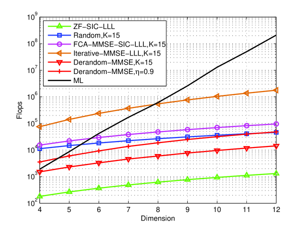
Figure 5: Complexity comparison in flops for a MIMO system using 64-QAM at SNR per bit = 17dB.

Based on the upper bound of the sphere radius $R$ in LSD, derandomized sampling algorithm can also be applied to implement soft-out decoding through sampling all the lattice points within $R$. Hence, according to (51), let $r=\sqrt{n}\sigma$, the derandomized sampling algorithm will achieve near-MAP performance even with lattice points in $\mathcal{C}_{1}$ only. Therefore, we have

$$\sqrt{\frac{2n}{\rho_{\text{o}}}}\ \text{min}_{i}r_{i,i}=\sqrt{n}\sigma$$ (57)

and

$$\rho_{\text{o}}=\frac{2\ \text{min}_{i}^{2}r_{i,i}}{\sigma^{2}}.$$ (58)

By substituting (58) into (32), the corresponding sample size $K$ can be derived as

$$K=\frac{1}{2}\left(\frac{2e\hskip 1.00006pt\text{min}_{i}^{2}r_{i,i}}{\sigma^{2}}\right)^{\left(\frac{n\sigma^{2}}{\text{min}_{i}^{2}r_{i,i}}\right)}.$$ (59)

Obviously, with the increment of $K$, more lattice points will be sampled and the corresponding sphere radius $r$ also increases gradually leading to further performance improvement. Note that the total sampling probability shown in (43) could also be used to reveal this flexible trade-off. As for achieving near-MAP performance, we emphasize that the required sample size $K$ of the derandomized sampling algorithm is significantly less than the value shown in (59). The reasons are two-fold: the derivation is based on a loose upper bound of $r$ shown in (53), and the contribution of set $\mathcal{C}_{2}$ which also contains sampled lattice points is not considered. Nevertheless, it provides a straightforward way of showing the trade-off in soft-output decoding with respect to $K$. Actually, with a moderate value of $K$, desirable performance gain in a low complexity burden can be achieved, as will be shown in simulation results.

V Simulation Results

In this section, performance and complexity of the derandomized sampling algorithm in MIMO systems are studied. Here, the $i$-th entry of the transmitted signal x, denoted as $x_{i}$, is the modulation symbol taken independently from a $Q^{2}$-QAM constellation $\mathcal{X}$ with Gray mapping. We assume a flat fading environment, the channel matrix $\mathbf{H}$ contains uncorrelated complex gaussian fading gains with unit variance and remains constant over each frame duration. Let $E_{b}$ represents the average power per bit at the receiver, then $E_{b}/N_{0}=n/(\text{log}_{2}(M)\sigma^{2})$ holds where $M$ is the modulation level and $\sigma^{2}$ is the noise power.

Fig. 4 shows the bit error rate (BER) of the derandomized sampling decoding compared with other decoding schemes in a $10\times 10$ uncoded MIMO system with 64-QAM. Clearly, sampling decoding schemes have considerable gains over the lattice-reduction-aided SIC. Compared to the fixed candidates algorithm (FCA) in [12] and iterative list decoding in [24] with 30 samples, sampling decoding algorithms offer not only the improved BER performance but also the promise of smaller sample size. As expected, derandomized sampling decoding achieves better BER performance than randomized sampling decoding with the same $K$. Specifically, the gain in MMSE schemes with $K=15$ is approximately 1 dB for a BER of $10^{-4}$. With the increment of $K$, the BER performance improves gradually. Observe that with $\eta=0.9$ ($K$=73), the performance of the derandomized sampling algorithm suffers negligible loss compared with ML. Therefore, with a moderate $K$, derandomized sampling decoding could achieve near-ML performance.

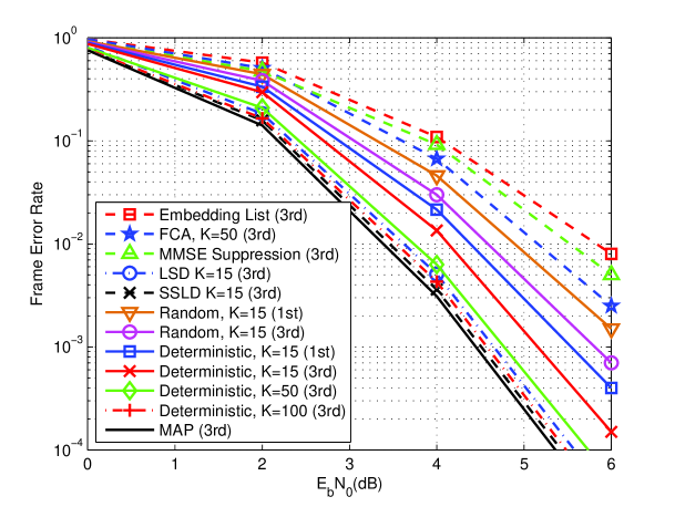
Figure 6: Frame error rate versus average SNR per bit in the coded $8\times 8$ MIMO BICM-IDD system with a rate-1/2 LDPC code of codeword length 256 using 4-QAM.

Fig. 5 shows the complexity comparison of the derandomized sampling algorithm with other schemes in different dimensions. It is clearly seen that in a 64-QAM MIMO system for the fixed SNR ($E_{b}/N_{0}=17$ dB), the derandomized sampling algorithm needs much lower average flops than other decoding schemes with the same size $K$. This can be interpreted as reducing the computation in sampling procedures by removing all the unnecessary repetitions. Even for a large $K=73$ $(\eta=0.9)$, the complexity is still lower than that of the randomized sampling algorithm with $K=15$. Consequently, better BER performance and less complexity requirement make derandomized sampling algorithm very promising for lattice decoding.

Fig. 6 shows the frame error rate for a coded $8\times 8$ MIMO BICM-IDD system with 4-QAM, using a rate-1/2, irregular (256,128,3) low-density parity-check (LDPC) code of codeword length 256 (i.e., 128 information bits). Each codeword spans one channel realization and a random bit interleaver is used. The parity check matrix is randomly constructed, but cycles of length 4 are eliminated. The maximum number of decoding iterations for LDPC is set at 50. Clearly, after three iterations between MIMO detector and SISO decoder in IDD, the proposed sampling algorithm with $K=15$ performs better than FCA, MMSE suppression [27], and Embedding list [28]. To achieve a better comparison, performance of both sampling algorithms with $K=15$ after one iteration are also given. As expected, derandomized sampling algorithm always achieves better FER performance than randomized sampling algorithm under the same iteration. Note that there is no significant performance gain after more than three iterations in IDD receivers. It is observed that the LSD in [9] and shifted sphere list deocding (SSLD) in [14] with sample size $K=15$ achieve near-MAP performance. However, due to the application of sphere decoding, their complexity are high and increase exponentially with the size of sphere radius and system dimensions leading them impractical. It is also shown that the performance gap between the proposed algorithm and MAP decreases with the increment of $K$ and near-MAP performance is achieved by derandomized sampling algorithm with a moderate size $K=100$. By adjusting $K$, the whole system enjoys a flexible trade-off between performance and complexity.

VI Conclusions

In this paper, we proposed a derandomized algorithm to address issues in sampling algorithms caused by randomization, which holds great potential in both lattice decoding and soft-output decoding. By setting a probability threshold to perform the sampling, the whole sampling procedure becomes deterministic. We demonstrated that the proposed derandomized sampling algorithm outperforms the randomized sampling algorithm with much lower complexity and derived the optimal parameter $A$ which maximizes the decoding radius $R_{\text{Derandomized}}$ for the best decoding performance. To accomplish the trade-off in lattice decoding, the upper bound on the sample size $K$ corresponding to near-ML performance was also given. Furthermore, we found that the proposed derandomized sampling algorithm is quite suitable for soft-output decoding through sampling a list of lattice points around the ML estimate. According to the analysis, we demonstrated that the derandomized sampling algorithm is capable of achieving near-MAP performance with a moderate size $K$. Therefore, by varying $K$, the decoder enjoys a flexible trade-off between performance and complexity in both lattice decoding and soft-output decoding.

References

- [1] L. Babai, “On Lovász’ lattice reduction and the nearest lattice point problem,” Combinatorica, vol. 6, no. 1, pp. 1–13, 1986.
- [2] L. Luzzi, G. Othman, and J. Belfiore, “Augmented lattice reduction for low-complexity MIMO decoding,” IEEE Trans. Wireless Commun., vol. 9, pp. 2853–2859, Sep. 2010.
- [3] D. Wubben, R. Bohnke, V. Kuhn, and K. D. Kammeyer, “Near-maximum-likelihood detection of MIMO systems using MMSE-based lattice reduction,” in Proc. IEEE Int. Conf. Commun.(ICC’04), Paris, France, Jun. 2004, pp. 798–802.
- [4] E. Agrell, T. Eriksson, A. Vardy, and K. Zeger, “Closest point search in lattices,” IEEE Trans. Inform. Theory, vol. 48, no. 8, pp. 2201–2214, Aug. 2002.
- [5] Y. H. Gan, C. Ling, and W. H. Mow, “Complex lattice reduction algorithm for low-complexity full-diversity MIMO detection,” IEEE Trans. Signal Process., vol. 57, no. 7, pp. 2701–2710, Jul. 2009.
- [6] J. Jalden and P. Elia, “DMT optimality of LR-aided linear decoders for a general class of channels, lattice designs, and system models,” IEEE Trans. Inform. Theory, vol. 56, no. 10, pp. 4765–4780, Oct. 2010.
- [7] C. Ling, “On the proximity factors of lattice reduction-aided decoding,” IEEE Trans. Signal Process., vol. 59, no. 6, pp. 2795–2808, Jun. 2011.
- [8] M. O. Damen, H. Gamal, and G. Caire, “On maximum-likelihood detection and the search for the closest lattice point,” IEEE Trans. Inform. Theory, vol. 49, pp. 2389–2401, Oct. 2003.
- [9] B. M. Hochwald and S. ten Brink, “Achieving near-capacity on a multiple-antenna channel,” IEEE Trans. Commun., vol. 51, no. 3, pp. 389 – 399, Mar. 2003.
- [10] H. Vikalo, B. Hassibi, and T. Kailath, “Iterative decoding for MIMO channels via modified sphere decoding,” IEEE Trans. Wireless Commun., vol. 3, no. 6, pp. 2299 – 2311, Nov. 2004.
- [11] P. Silvola, K. Hooli, and M. Juntti, “Suboptimal soft-output map detector with lattice reduction,” IEEE Signal Process. Lett., vol. 13, no. 6, pp. 321 – 324, Jun. 2006.
- [12] W. Zhang and X. Ma, “Low-complexity soft-output decoding with lattice-reduction-aided detectors,” IEEE Trans. Commun., vol. 58, no. 9, pp. 2621–2629, Sep. 2010.
- [13] D. Milliner and J. Barry, “A lattice-reduction-aided soft detector for multiple-input multiple-output channels,” in Proc. IEEE Globecom’06, Nov. 2006, pp. 1–5.
- [14] J. Boutros, N. Gresset, L. Brunel, and M. Fossorier, “Soft-input soft-output lattice sphere decoder for linear channels,” in Proc. IEEE GLOBECOM, San Francisco, Dec. 2003, pp. 1583–1587.
- [15] J. Lee, B. Shim, and I. Kang, “Soft-input soft-output list sphere detection with a probabilistic radius tightening,” IEEE Trans. Wireless Commun., vol. 11, no. 8, pp. 2848 –2857, Aug. 2012.
- [16] S. Liu, C. Ling, and D. Stehle, “Decoding by sampling: a randomized lattice algorithm for bounded distance decoding,” IEEE Trans. Inform. Theory, vol. 57, pp. 5933–5945, Sep. 2011.
- [17] P. Klein, “Finding the closest lattice vector when it is unusually close,” SIAM Symposium on Discrete Algorithms, pp. 937–941, ACM, 2000.
- [18] E. Larsson and J. Jalden, “Fixed-complexity soft MIMO detection via partial marginalization,” IEEE Trans. Signal Process., vol. 56, pp. 3397–3407, Aug. 2008.
- [19] R. Wang and G. B. Giannakis, “Approaching MIMO channel capacity with soft detection based on hard sphere decoding,” IEEE Trans. Commun., vol. 54, no. 4, pp. 587 – 590, Apr. 2006.
- [20] C. Studer and H. Bolcskei, “Soft-input soft-output single tree-search sphere decoding,” IEEE Trans. Inform. Theory, vol. 56, no. 10, pp. 4827 –4842, Oct. 2010.
- [21] R. Gowaikar and B. Hassibi, “Statistical pruning for near-maximum likelihood decoding,” IEEE Trans. Signal Process., vol. 55, no. 6, pp. 2661–2675, Jun. 2007.
- [22] W. Zhao and G. Giannakis, “Sphere decoding algorithms with improved radius search,” IEEE Trans. Commun., vol. 53, no. 7, pp. 1104–1109, Jul. 2005.
- [23] B. Shim and I. Kang, “Sphere decoding with a probabilistic tree pruning,” IEEE Trans. Signal Process., vol. 56, no. 10, pp. 4867–4878, Oct. 2008.
- [24] T. Shimokawa and T. Fujino, “Iterative lattice reduction aided MMSE list detection in MIMO system,” in Proc. IEEE International Conference on Advanced Technologies for Communications, Oct. 2008, pp. 50–54.
- [25] J. Jalden, L. Barbero, B. Ottersten, and J. Thompson, “The error probability of the fixed-complexity sphere decoder,” IEEE Trans. Signal Process., vol. 57, pp. 2711–2720, Jul. 2009.
- [26] W. Banaszczyk, “New bounds in some transference theorems in the geometry of numbers,” in Math. Ann. 296, 1993, pp. 625–635.
- [27] A. Matache, C. Jones, and R. D. Wesel, “Reduced complexity MIMO detectors for LDPC coded systems,” in Proc. IEEE Military Commun. Conf., Monterey, USA, 2004, pp. 1073–1079.
- [28] L. Luzzi, D. Stehle, and C. Ling, “Decoding by embedding: correct decoding radius and DMT optimality,” IEEE Trans. Inform. Theory, vol. 59, no. 5, pp. 2960–2973, 2013.