Abstract

The type II seesaw mechanism for neutrino mass generation usually makes use of one complex scalar triplet. The collider signature of the doubly-charged scalar, the most striking feature of this scenario, consists mostly in decays into same-sign dileptons or same-sign $W$ boson pairs. However, certain scenarios of neutrino mass generation, such as those imposing texture zeros by a symmetry mechanism, require at least two triplets in order to be consistent with the type II seesaw mechanism. We develop a model with two such complex triplets and show that, in such a case, mixing between the triplets can cause the heavier doubly-charged scalar mass eigenstate to decay into a singly-charged scalar and a $W$ boson of the same sign. Considering a large number of benchmark points with different orders of magnitude of the $\Delta L=2$ Yukawa couplings, chosen in agreement with the observed neutrino mass and mixing pattern, we demonstrate that $H^{++}_{1}\rightarrow H^{+}_{2}W^{+}$ can have more than 99% branching fraction in the cases where the vacuum expectation values of the triplets are small. It is also shown that the above decay allows one to differentiate a two-triplet case at the LHC, through the ratios of events in various multi-lepton channels.

1 Introduction

It is by and large agreed that the Large Hadron Collider (LHC) has discovered the Higgs boson predicted in the standard electroweak theory, or at any rate a particle with close resemblance to it [1, 2]. At the same time, driven by both curiosity and various physics motivations, physicists have been exploring the possibility that the scalar sector of elementary particles contains more members than just a single $SU(2)$ doublet. A rather well-motivated scenario often discussed in this context is one containing at least one complex scalar $SU(2)$ triplet of the type $(\Delta^{++},\Delta^{+},\Delta^{0})$ [3]. A small vacuum expectation value of the neutral member of the triplet, constrained as it is by the $\rho$-parameter, can lead to Majorana masses for neutrinos, driven by $\Delta L=2$ Yukawa interactions of the triplet. Such mass generation does not require any right-handed neutrino, and this is the quintessential principle of the type II seesaw mechanism [4, 5].

One of the most phenomenologically striking features of this mechanism is the occurrence of a doubly-charged scalar. Its signature at TeV scale colliders is expected to be seen, if the triplet masses are not too far above the electroweak symmetry breaking scale. The most conspicuous signal consists in the decay into a pair of same-sign leptons, i.e. $\Delta^{++}\rightarrow\ell^{+}\ell^{+}$. The same-sign dilepton invariant mass peaks resulting from this make the doubly-charged scalar show up rather conspicuously. Alternatively, the decay into a pair of same-sign $W$ bosons, i.e. $\Delta^{++}\rightarrow W^{+}W^{+}$, is dominant in a complementary region of the parameter space, which—though more challenging from the viewpoint of background elimination—can unravel a doubly-charged scalar [6].

In this paper, we shall discuss the situation where a third decay channel, namely a doubly-charged scalar decaying into a singly-charged scalar and a $W$ of the same sign, is dominant or substantial. Such a decay mode is usually suppressed, since the underlying $SU(2)$ invariance implies relatively small mass splitting among the members of a triplet. However, when several triplets of a similar nature are present and mixing among them is allowed, a transition of the above kind is possible between two scalar mass eigenstates. Apart from being interesting in itself, several scalar triplets naturally occur in models for neutrino masses and lepton mixing based on the type II seesaw mechanism. In particular, it has been shown that in such a scenario a realization of viable neutrino mass matrices with two texture zeros [7], using symmetry arguments [9], requires two or three scalar triplets [10]. In this paper, we take up the case of two coexisting triplets. We demonstrate that in such cases one doubly-charged state can often decay into a singly-charged state and a $W$ of identical charge. This is not surprising, because each of the two erstwhile studied decay modes is controlled by parameters that are rather suppressed. In the case of $\Delta^{++}\rightarrow\ell^{+}\ell^{+}$, the amplitude is proportional to the $\Delta L=2$ Yukawa coupling, while for $\Delta^{++}\rightarrow W^{+}W^{+}$, it is driven by the triplet vacuum expectation value (VEV). The restrictions from neutrino masses as well as precision electroweak constraints makes both of these rates rather small. On the other hand, in the scenario with two scalar triplets with charged mass eigenstates $H^{++}_{k}$ and $H^{+}_{l}$ ($k,l=1,2$), the decay amplitude for $H_{1}^{++}\rightarrow H_{2}^{+}W^{+}$, if kinematically allowed, is controlled by the $SU(2)$ gauge coupling. Therefore, if one identifies regions of the parameter space where it dominates, one needs to devise new search strategies at the LHC [11], including ways of eliminating backgrounds.

We note that the mass parameters of the two triplets, on which no phenomenological restrictions exist, are a priori unrelated and, therefore, as a result of mixing between the two triplets, the heavier doubly-charged state can decay into a lighter, singly-charged state and a real $W$ over a wide range of the parameter space. In that range it is expected that this decay channel dominates for the heavier doubly-charged state. By choosing a number of benchmark points, we demonstrate that this is indeed the case.

In section 2, we present a summary of the model with a single triplet and explain why the decay $\Delta^{++}\rightarrow\Delta^{+}W^{+}$ is disfavoured there. The details of a two-triplet scenario, including the scalar potential and the composition of the physical states, are presented in section 3. We select several benchmark points and show the decay patterns of the corresponding doubly-charged scalars in section 4, where their production rates at the LHC are also presented. We point out the usefulness of $H_{1}^{++}\rightarrow H_{2}^{+}W^{+}$ at the LHC in the context of our model with two scalar triplets in section 5. We summarise and conclude in section 6. In appendix A the input parameters for the benchmark points are listed while appendix B contains the formulas for the decay rates of the doubly-charged scalars.

2 The scenario with a single triplet

In this section we perform a quick recapitulation of the scenario with a single triplet field, in addition to the usual Higgs doublet $\phi$, using the notation of [12]. The Higgs triplet $\Delta=(\Delta^{++},\Delta^{+},\Delta^{0})$ is represented by the $2\times 2$ matrix

$$\Delta=\left(\begin{array}[]{cc}\Delta^{+}&\sqrt{2}\Delta^{++}\\ \sqrt{2}\Delta^{0}&-\Delta^{+}\end{array}\right).$$ (1)

The VEVs of the doublet and the triplet are given by

$$\langle\phi\rangle_{0}=\frac{1}{\sqrt{2}}\left(\begin{array}[]{c}0\\ v\end{array}\right)\quad\mbox{and}\quad\langle\Delta\rangle_{0}=\left(\begin{array}[]{cc}0&0\\ w&0\end{array}\right),$$ (2)

respectively. Thus, the triplet VEV is obtained as $\langle\Delta^{0}\rangle=w/\sqrt{2}$ . The only doublet-dominated physical state that survives after the generation of gauge boson masses is a neutral scalar $H$.

The most general scalar potential involving $\phi$ and $\Delta$ can be written as

$$V(\phi,\Delta)\ =\hphantom{+}a\,\phi^{\dagger}\phi+\ \frac{b}{2}\,\mbox{Tr}\,(\Delta^{\dagger}\Delta)+\ c\,(\phi^{\dagger}\phi)^{2}+\ \frac{d}{4}\left(\,\mbox{Tr}\,(\Delta^{\dagger}\Delta)\right)^{2}$$

$$+\ \frac{e-h}{2}\phi^{\dagger}\phi\,\mbox{Tr}\,(\Delta^{\dagger}\Delta)+\ \frac{f}{4}\,\mbox{Tr}\,(\Delta^{\dagger}\Delta^{\dagger})\,\mbox{Tr}\,(\Delta\Delta)$$

$$+\ h\phi^{\dagger}\Delta^{\dagger}\Delta\phi+\left(t\,\phi^{\dagger}\Delta\tilde{\phi}+\mbox{H.c.}\right),$$ (3)

where $\tilde{\phi}\equiv i\tau_{2}\phi^{\ast}$. For simplicity, we assume both $v$ and $w$ to be real and positive, which requires $t$ to be real as well. In other words, all CP-violating effects are neglected in this study.

The choice $a<0$, $b>0$ ensures that the primary source of spontaneous symmetry breaking resides in the VEV of the scalar doublet. Without any loss of generality, we assume the following orders of magnitude for the parameters in the potential:

$$a,\>b\sim v^{2};\quad c,\>d,\>e,\>f,\>h\sim 1;\quad|t|\ll v.$$ (4)

Such a choice is motivated by

1. proper fulfillment of the electroweak symmetry breaking conditions,

2. the need to have $w\ll v$ small due to the $\rho$-parameter constraint,

3. the need to keep doublet-triplet mixing low in general, and

4. the urge to ensure perturbativity of all quartic couplings.

The mass Lagrangian for the singly-charged scalars in this model is given by

$$\mathcal{L}^{\pm}_{S}=-(H^{-},\phi^{-})\mathcal{M}_{+}^{2}\left(\begin{array}[]{c}H^{+}\\ \phi^{+}\end{array}\right)$$ (5)

with

$$\mathcal{M}_{+}^{2}=\left(\begin{array}[]{cc}(q+h/2)v^{2}&\sqrt{2}v(t-wh/2)\\ \sqrt{2}v(t-wh/2)&2(q+h/2)w^{2}\end{array}\right)\quad\mbox{and}\quad q=\frac{|t|}{w}.$$ (6)

The field $\phi^{+}$ is the charged component of the doublet scalar field of the Standard Model (SM). One of the eigenvalues of this matrix is zero corresponding to the Goldstone boson which gives mass to the $W$ boson. The mass-squared of the singly-charged physical scalar is obtained as

$$m^{2}_{\Delta^{+}}=\left(q+\frac{h}{2}\right)(v^{2}+2w^{2}),$$ (7)

whereas the corresponding expression for the doubly-charged scalar is

$$m^{2}_{\Delta^{++}}=(h+q)v^{2}+2fw^{2}.$$ (8)

Thus, in the limit $w\ll v$, we obtain

$$m^{2}_{\Delta^{++}}-m^{2}_{\Delta^{+}}\simeq{\frac{h}{2}}v^{2}.$$ (9)

It is obvious from the above that a substantial mass splitting between $\Delta^{++}$ and $\Delta^{+}$ is in general difficult. This is clear from Figure 1 where we plot the mass difference between the two states for different values of $h$. Sufficient splitting, so as to enable the decay $\Delta^{++}\rightarrow\Delta^{+}W^{+}$ to take place with appreciable branching ratio, will require $h\simeq 1$, $m_{\Delta^{++}}\lesssim 250$ GeV and a correspondingly smaller $m_{\Delta^{+}}$. The limits from LEP and Tevatron disfavour triplet states with such low masses. Thus one concludes that the phenomenon of the doubly-charged scalar decaying into a singly-charged one and a $W$ is very unlikely.

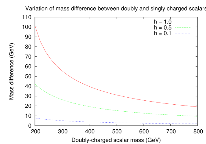
Figure 1: Variation of mass difference between the doubly and singly-charged scalars, for various values of the parameter $h$.

3 A two Higgs triplet scenario

There may, however, be some situations where a single triplet is phenomenologically inadequate. This happens, for example, when one tries to impose texture zeros in the neutrino mass matrix within a type II seesaw framework by using Abelian symmetries [10]. Having this is in mind, we venture into a model consisting of one complex doublet and two $Y=2$ triplet scalars $\Delta_{1}$, $\Delta_{2}$, both written as 2$\times$2 matrices:

$$\Delta_{1}=\left(\begin{array}[]{cc}\delta_{1}^{+}&\sqrt{2}\delta_{1}^{++}\\ \sqrt{2}\delta_{1}^{0}&-\delta_{1}^{+}\end{array}\right)\quad\mbox{and}\quad\Delta_{2}=\left(\begin{array}[]{cc}\delta_{2}^{+}&\sqrt{2}\delta_{2}^{++}\\ \sqrt{2}\delta_{2}^{0}&-\delta_{2}^{+}\end{array}\right).$$ (10)

The VEVs of the scalar triplets are given by

$$\langle\Delta_{1}\rangle_{0}=\left(\begin{array}[]{cc}0&0\\ w_{1}&0\end{array}\right)\quad\mbox{and}\quad\langle\Delta_{2}\rangle_{0}=\left(\begin{array}[]{cc}0&0\\ w_{2}&0\end{array}\right).$$ (11)

The VEV of the Higgs doublet is as usual given by equation (2).

The scalar potential in this model involving $\phi$, $\Delta_{1}$ and $\Delta_{2}$ can be written as

$$V(\phi,\Delta_{1},\Delta_{2})=$$ (12)

$$a\,\phi^{\dagger}\phi+\frac{1}{2}\,b_{kl}\,\mbox{Tr}\,(\Delta_{k}^{\dagger}\Delta_{l})+c(\phi^{\dagger}\phi)^{2}+\frac{1}{4}\,d_{kl}\left(\,\mbox{Tr}\,(\Delta_{k}^{\dagger}\Delta_{l})\right)^{2}$$

$$+\frac{1}{2}\,(e_{kl}-h_{kl})\,\phi^{\dagger}\phi\,\mbox{Tr}\,(\Delta_{k}^{\dagger}\Delta_{l})+\frac{1}{4}\,f_{kl}\,\mbox{Tr}\,(\Delta_{k}^{\dagger}\Delta_{l}^{\dagger})\,\mbox{Tr}\,(\Delta_{k}\Delta_{l})$$

$$+h_{kl}\,\phi^{\dagger}\Delta_{k}^{\dagger}\Delta_{l}\phi+g\,\mbox{Tr}\,(\Delta_{1}^{\dagger}\Delta_{2})\,\mbox{Tr}\,(\Delta_{2}^{\dagger}\Delta_{1})+g^{\prime}\,\mbox{Tr}\,(\Delta_{1}^{\dagger}\Delta_{1})\,\mbox{Tr}\,(\Delta_{2}^{\dagger}\Delta_{2})$$

$$+\left(t_{k}\,\phi^{\dagger}\Delta_{k}\tilde{\phi}+\mbox{H.c.}\right),$$

where summation over $k,l=1,2$ is understood. This potential is not the most general one, as we have omitted some of the quartic terms. This is justified in view of the scope of this paper, as laid out in the introduction. Moreover, due to the smallness of the triplet VEVs, the quartic terms are not important numerically for the mass matrices of the scalars.

As in the case with a singlet triplet, we illustrate our main point here taking all the VEVs $v,w_{1},w_{2}$ as real and positive, and with real values for $t_{1},t_{2}$ as well. Again, the following orders of magnitude for the parameters in the potential are assumed:

$$a,\>b_{kl}\sim v^{2};\quad c,\>d_{kl},\>e_{kl},\>h_{kl},\>f_{kl},\>g,\>g^{\prime}\sim 1;\quad|t_{k}|\ll v.$$ (13)

We also confine ourselves to cases where $w_{1},w_{2}\ll v$, keeping in mind the constraint on the $\rho$-parameter.

In general, the scalar potential (12) can only be treated numerically. However, since the triplet VEVs $w_{k}$ are small (we will have $w_{k}\lesssim 1$ GeV in our numerical part), it should be a good approximation to drop the quartic terms in the scalar triplets. In the following we will discuss the VEVs and the mass matrices of the doubly and singly-charged scalars in this approximation, so that our broad conclusions are transparent. However, the numerical results presented in section 4 are obtained using the full potential (12), including even the effects of the small triplet VEVs. We find that the results are in very good accordance with the approximation.

For the sake of a convenient notation we define the following $2\times 2$ matrices and vectors:

$$B=(b_{kl}),\quad E=(e_{kl}),\quad H=(h_{kl}),\quad t=\left(\begin{array}[]{c}t_{1}\\ t_{2}\end{array}\right),\quad w=\left(\begin{array}[]{c}w_{1}\\ w_{2}\end{array}\right).$$ (14)

With this notation the conditions for a stationary point of the potential are given by

$$\left(B+\frac{v^{2}}{2}\left(E-H\right)\right)w+v^{2}\,t = 0,$$ (15)

$$a+cv^{2}+\frac{1}{2}w^{T}(E-H)w+2\,t\cdot w = 0,$$ (16)

where we have used the notation $t\cdot w=\sum_{k}t_{k}w_{k}$. These two equations are exact if one neglects all terms quartic in the triplet VEVs in $V_{0}\equiv V(\langle\phi\rangle_{0},\langle\Delta\rangle_{0})$. In equation (16) we have already divided by $v$, assuming $v\neq 0$. Using equation (15), the small VEVs $w_{k}$ are obtained as

$$w=-v^{2}\left(B+\frac{1}{2}v^{2}(E-H)\right)^{-1}t.$$ (17)

Now we discuss the mass matrices of the charged scalars. A glance at the scalar potential equation (12)—neglecting quartic terms in the triplet scalars—reveals that the first two lines of $V$ make no difference between the singly and doubly-charged scalars. Thus, the difference in the respective mass matrices originates in the terms of the third line. The mass matrix of the doubly-charged scalars is obtained as

$$\mathcal{M}^{2}_{++}=B+\frac{v^{2}}{2}\left(E+H\right).$$ (18)

As for the singly-charged fields $\Delta^{+}_{k}$, one has to take into account that they can mix with $\phi^{+}$ of the Higgs doublet. Writing the mass term as

$$-\mathcal{L}^{\pm}_{S}=\left(\delta^{-}_{1},\delta^{-}_{2},\phi^{-}\right)\mathcal{M}^{2}_{+}\left(\begin{array}[]{c}\delta^{+}_{1}\\ \delta^{+}_{2}\\ \phi^{+}\end{array}\right)+\mbox{H.c.},$$ (19)

equation (12) leads to

$$\mathcal{M}^{2}_{+}=\left(\begin{array}[]{cc}B+\frac{v^{2}}{2}\,E&\sqrt{2}v\left(t-Hw/2\right)\\ \sqrt{2}v\left(t-Hw/2\right)^{\dagger}&a+cv^{2}+\frac{1}{2}w^{T}(E+H)w\end{array}\right).$$ (20)

Obviously, this mass matrix has to have an eigenvector with eigenvalue zero which corresponds to the would-be-Goldstone boson. Indeed, using equations (15) and (16), we find

$$\mathcal{M}^{2}_{+}\left(\begin{array}[]{c}v_{T}\\ v/\sqrt{2}\end{array}\right)=0,$$ (21)

which serves as a consistency check.

Note that the matrix $B$ largely controls the mass of the triplet scalars and the order of magnitude of its elements (or of its eigenvalues) is expected to be a little above the electroweak scale, represented by $v\simeq 246$ GeV. On the other hand, the quantities $t_{k}$ trigger the small triplet VEVs, so they should be considerably smaller than the electroweak scale. Therefore, in a rough approximation one could neglect the $t_{k}$ and the triplet VEVs in the mass matrix $\mathcal{M}^{2}_{+}$. In that limit, also $a+cv^{2}=0$ and the charged would-be-Goldstone boson consists entirely of $\phi^{+}$, without mixing with the $\delta^{+}_{k}$.

The mass matrices (19) and (20) are diagonalized by

$$U^{\dagger}\mathcal{M}^{2}_{++}U=\mbox{diag}\,(M^{2}_{1},M^{2}_{2})\quad\mbox{and}\quad V^{\dagger}\mathcal{M}^{2}_{+}V=\mbox{diag}\,(\mu_{1}^{2},\mu_{2}^{2},0),$$ (22)

respectively, with

$$\left(\begin{array}[]{c}\delta^{++}_{1}\\ \delta^{++}_{2}\end{array}\right)=U\left(\begin{array}[]{c}H^{++}_{1}\\ H^{++}_{2}\end{array}\right),\quad\left(\begin{array}[]{c}\delta^{+}_{1}\\ \delta^{+}_{2}\\ \phi^{+}\end{array}\right)=V\left(\begin{array}[]{c}H^{+}_{1}\\ H^{+}_{2}\\ G^{+}\end{array}\right).$$ (23)

We have denoted the fields with definite mass by $H^{++}_{k}$ and $H^{+}_{k}$, and $G^{+}$ is the charged would-be-Goldstone boson.

The gauge Lagrangian relevant for the decays considered in this paper is given by

$$\mathcal{L}_{\mathrm{gauge}} = ig\sum_{k=1}^{2}\left[\delta^{-}_{k}(\partial^{\mu}\delta^{++}_{k})-(\partial^{\mu}\delta^{-}_{k})\,\delta^{++}_{k}\right]W_{\mu}^{-}$$ (24)

$$-\frac{g^{2}}{\sqrt{2}}\sum_{k=1}^{2}w_{k}W^{-}_{\mu}{W^{-}}^{\mu}\delta_{k}^{++}+\mbox{H.c.}$$

Here $g$ is the $SU(2)$ gauge coupling constant. Inserting equation (23) into this Lagrangian allows us to compute the decay rates of $H_{1}^{++}\to H_{2}^{+}W^{+}$ and $H_{k}^{++}\to W^{+}W^{+}$ ($k=1,2$). The corresponding formulas are found in appendix B.

The $\Delta L=2$ Yukawa interactions between the triplets and the leptons are

$$\mathcal{L}_{Y}=\frac{1}{2}\,\sum_{k=1}^{2}h^{(k)}_{ij}L^{T}_{i}C^{-1}i\tau_{2}\Delta_{k}L_{j}+\mbox{H.c.},$$ (25)

where $C$ is the charge conjugation matrix, the $h^{(k)}_{ij}$ are the symmetric Yukawa coupling matrices of the triplets $\Delta_{k}$, and the $i,j$ are the summation indices over the three neutrino flavours. The $L_{i}$ denote the left-handed lepton doublets.

The neutrino mass matrix is generated from equation (25) when the triplets acquire VEVs:

$$(M_{\nu})_{ij}=h^{(1)}_{ij}w_{1}+h^{(2)}_{ij}w_{2}.$$ (26)

This connects the Yukawa coupling constants $h^{(1)}_{ij}$, $h^{(2)}_{ij}$ and the triplet VEVs $w_{1}$, $w_{2}$, once the neutrino mass matrix is written down for a particular scenario. In our subsequent calculations, we proceed as follows. First of all, the neutrino mass eigenvalues are fixed according to a particular type of mass spectrum. In this work we illustrate our points, without any loss of generality, by resorting to normal hierarchy of the neutrino mass spectrum and setting the lowest neutrino mass eigenvalue to zero. Furthermore, using the observed central values of the various lepton mixing angles, the elements of the neutrino mass matrix $M_{\nu}$ can be found by using the equation

$$M_{\nu}=U{\hat{M}}_{\nu}U^{\dagger},$$ (27)

where $U$ is the PMNS matrix given by [16]

$$U=\left(\begin{array}[]{ccc}c_{12}c_{13}&s_{12}c_{13}&s_{13}e^{-i\delta}\\ -s_{12}c_{23}-c_{12}s_{23}s_{13}e^{i\delta}&c_{12}c_{23}-s_{12}s_{23}s_{13}e^{i\delta}&s_{23}c_{13}\\ s_{12}s_{23}-c_{12}c_{23}s_{13}e^{i\delta}&-c_{12}s_{23}-s_{12}c_{23}s_{13}e^{i\delta}&c_{23}c_{13}\end{array}\right)$$ (28)

and ${\hat{M}}_{\nu}$ is the diagonal matrix of the neutrino masses. In equation (27) we have dropped possible Majorana phases. One can use the recent global analysis of data to determine the various entries of $U$ [13]. We have taken the phase factor $\delta$ to be zero for simplicity. Then, using the central values of all angles, including that for $\theta_{13}$ as obtained from the recent Daya Bay and RENO experiments [14, 15], the left-hand side of equation (25) is completely known, at least in orders of magnitude. The actual mass matrix thus constructed has some elements at least one order of magnitude smaller than the others, thus suggesting texture zeros.

For each of the benchmark points used in the next section, $w_{1}$ and $w_{2}$, the VEVs of the two triplets, are determined by values of the parameters in the scalar potential. Of course, the coupling matrices $h^{(1)}$ and $h^{(2)}$ are still indeterminate. In order to evolve a working principle based on economy of free parameters, we fix the Yukawa coupling matrix $h^{(2)}$ by choosing one suitable value for all elements of the $\mu$–$\tau$ block and another value, a smaller one, for the rest of the matrix. That fixes all the elements of the other matrix. Although there is a degree of arbitrariness in such a method, we emphasize that it does not affect the generality of our conclusions, so long as we adhere to the wide choice of scenarios adopted in the next section, including both small and large values of the $\Delta L=2$ Yukawa couplings.

4 Benchmark points and doubly-charged scalar decays

Our purpose is to investigate the expected changes in the phenomenology of doubly-charged scalars when two triplets are present. In general, the two scalars of this kind, namely, $H^{++}_{1}$ and $H^{++}_{2}$ can both be produced at the LHC via the Drell-Yan process, which can have about 10% enhancement from the two-photon channel. They will, over a large region of the parameter space, have the following decays:

$$H^{++}_{1} \rightarrow \ell^{+}_{i}\ell^{+}_{j},$$ (29)

$$H^{++}_{1} \rightarrow W^{+}W^{+},$$ (30)

$$H^{++}_{1} \rightarrow H^{+}_{2}W^{+},$$ (31)

$$H^{++}_{2} \rightarrow \ell^{+}_{i}\ell^{+}_{j},$$ (32)

$$H^{++}_{2} \rightarrow W^{+}W^{+},$$ (33)

with $\ell_{i},\ell_{j}=e,\mu,\tau$ in equation (29). As we discussed in section 2, in the context of the single-triplet model the decay analogous to equation (31) is practically never allowed, unless the masses are very low. On the other hand, mixing between two triplets opens up situations where the mass separation between $H^{++}_{1}$ and $H^{+}_{2}$ kinematically allows the transition (31). Denoting the mass of $H_{k}^{++}$ by $M_{k}$ and that of $H_{k}^{+}$ by $\mu_{k}$ ($k=1,2$) and using the convention $M_{1}>M_{2}$ and $\mu_{1}>\mu_{2}$, this decay is possible if $M_{1}>\mu_{2}+m_{W}$. We demonstrate numerically that this can naturally happen, by considering three distinct regions of the parameter space and selecting four benchmark points (BPs) for each region.

We have seen that, in a model with a single triplet, the doubly-charged Higgs decays into either $\ell^{+}_{i}\ell^{+}_{j}$ or $W^{+}W^{+}$. The former is controlled by the $\Delta L=2$ coupling constants $h_{ij}$, while the latter is driven by the triplet VEV $w$. Since neutrino masses are given by $M_{\nu}=hw$, large ($\simeq 1$) values of $h_{ij}$ imply a small VEV $w$, and vice versa. Accordingly, assuming $h_{ij}\neq 0$, three regions in the parameter space can be identified, where one can have

1. $\Gamma(\Delta^{++}\rightarrow\ell^{+}_{i}\ell^{+}_{j})\ll\Gamma(\Delta^{++}\rightarrow W^{+}W^{+})$,

2. $\Gamma(\Delta^{++}\rightarrow\ell^{+}_{i}\ell^{+}_{j})\gg\Gamma(\Delta^{++}\rightarrow W^{+}W^{+})$,

3. $\Gamma(\Delta^{++}\rightarrow\ell^{+}_{i}\ell^{+}_{j})\sim\Gamma(\Delta^{++}\rightarrow W^{+}W^{+})$.

In the context of two triplets, we choose three different ‘scenarios’ in the same spirit, with similar relative rates of the two channels $H^{++}_{k}\rightarrow\ell^{+}_{i}\ell^{+}_{j}$ and $H^{++}_{k}\rightarrow W^{+}W^{+}$. Four BPs are selected for each such scenario through the appropriate choice of parameters in the scalar potential. The parameters for each BP are listed in appendix A. The resulting masses of the various physical scalar states are shown in tables 1 and 2. Although our study focuses mainly on the phenomenology of charged scalars, we also show the masses of the neutral scalars. It should be noted that the lightest CP-even neutral scalar, which is dominated by the doublet, has mass around 125 GeV for each BP.

All the twelve BPs (distributed among the three different scenarios) have $M_{1}$ sufficiently above $M_{2}$ to open up $H^{++}_{1}\rightarrow H^{+}_{2}W^{+}$. The branching ratios in different channels are of course dependent on the specific BP. We list all the branching ratios for $H^{++}_{1}$ and $H^{++}_{2}$ in table 3, together with their pair-production cross sections at the LHC with $\sqrt{s}=14$ TeV.

The cross sections and branching ratios have been calculated with the help of the package FeynRules (version 1.6.0) [17, 18], thus creating a new model file in CompHEP (version 2.5.4) [19]. CTEQ6L parton distribution functions have been used, with the renormalisation and factorisation scales set at the doubly-charged scalar mass. Using the full machinery of scalar mixing in this model, the decay widths into various channels have been obtained, for which the relevant expressions are presented in appendix B.

The results summarised in table 3 show that, for the decay of $H^{++}_{1}$, the channel $H^{+}_{2}W^{+}$ is dominant for two of the four BPs in scenario 1 and all four BPs in scenarios 2 and 3. This, in the first place, substantiates our claim that one may have to look for a singly-charged scalar in the final state that opens up when more than one doublet is present. This is because, for the BPs where $H^{++}_{1}\rightarrow H^{+}_{2}W^{+}$ dominates, the branching ratios for the other final states are far too small to yield any detectable rates.

5 Usefulness of $H_{1}^{++}\longrightarrow H_{2}^{+}W^{+}$ at the LHC

Table 3 contains the rates for pair-production of the heavier as well as the lighter doubly-charged scalar at the 14 TeV run of the LHC. A quick look at these rates revals that, for the heavier of the doubly-charged scalars, it varies from about 1.4 fb to 3.6 fb, for masses ranging approximately between 400 and 550 GeV. Therefore, as can be read off from table 3, for ten of our twelve BPs, an integrated luminosity of about 500 fb^-1 is likely to yield about $700$ to $1800$ events of the $H^{+}_{2}W^{+}H^{-}_{2}W^{-}$ type. Keeping in mind the fact that $H^{+}_{2}$ mostly decays in the channel $H^{+}_{2}\rightarrow\ell^{+}\bar{\nu}_{\ell}$, such final states should prima facie be observed at the LHC, although event selection strategies of a very special nature may be required to distinguish the $H^{+}_{2}$ from a $W^{+}$ decaying into $\ell^{+}\nu_{\ell}$.

The primary advantage of focusing on the channel $H_{1}^{++}\longrightarrow H_{2}^{+}W^{+}$ is that it helps one in differentiating between the two kinds of type II cases, namely those containing one and two scalar triplets, respectively. In order to emphasize this point, we summarize below the result of a simulation in the context of the 14 TeV run of the LHC. For our simulation, the amplitudes have been computed using the package Feynrules (version 1.6.0), with the subsequent event generation through MadGraph (version 5.12) [20], and showering with the help of PYTHIA 8.0. CTEQ6L parton distribution functions have been used.

We compare the two-triplet case with the single-triplet case. In the first case, there are two doubly charged scalars, and one has contributions from both $H_{1}^{\pm\pm}$ and $H_{2}^{\pm\pm}$ to the leptonic final states following their Drell-Yan production. While the former, in the chosen benchmark points, decays into $H_{1}^{\pm}W^{\pm}$, the latter goes either to a same-sign $W$-pair or to same-sign dileptons. If one considers two, three and four-lepton final states with missing transverse energy (MET), there will be contributions from both of the doubly-charged scalars, with appropriate branching ratios, combinatoric factors and response to the cuts imposed. We have carried out our analysis with a set of cuts listed in table 4, which are helpful in suppressing the standard model backgrounds. Thus one can define the following ratios of events emerging after the application of cuts:

$$r_{1}=\frac{\sigma(4\ell+\mathrm{MET})}{\sigma(3\ell+\mathrm{MET})},\qquad r_{2}=\frac{\sigma(4\ell+\mathrm{MET})}{\sigma(2\ell+\mathrm{MET})}.$$ (34)

The values of these ratios for the three scenarios of BP 3 are presented in table 5. In each case, the ratios for the two-triplet case is presented alongside the corresponding single-triplet case, with the mass of the doubly charged scalar in the latter case being close to that of the lighter state $H_{2}^{\pm\pm}$ in the former. Both of the situations where, in the later case, the doubly charged scalar decays dominantly into either $W^{\pm}W^{\pm}$ or $\ell^{\pm}\ell^{\pm}$ are represented in our illustrative results. One can clearly notice from the results (which apply largely to our other benchmark points as well) that both $r_{1}$ and $r_{2}$ remain substantially larger in the two-triplet case as compared to the single-triplet case. One reason for this is an enhancement via the combinatoric factors in the two-triplet case. However, the more important reason is that the 4$\ell$ events survive the MET cut with greater efficiency. In the single-triplet case, the survival rate efficiency is extremely small when $H^{\pm\pm}$ decays mainly into same-sign dileptons, the MET coming mostly from energy-momentum mismeasurement (as a result of lepton energy smearing) or initial and final-state radiation. In the two-triplet case, on the other hand, the decay $H_{1}^{++}\longrightarrow H_{2}^{+}W^{+}$ leaves ample scope for having MET in $W$-decays as well as in the decay $H_{2}^{+}\longrightarrow\ell^{+}\bar{\nu}_{\ell}$, thus leading to substantially higher cut survival efficiency. Thus, from an examination of such numbers as those presented in table 5, one can quite effectively use the channel $H_{1}^{++}\longrightarrow H_{2}^{+}W^{+}$ to distinguish a two-triplet case from a single-triplet case, provided the heavier doubly-charged state is within the kinematic reach of the LHC.

	Mass (GeV)	BP 1	BP 2	BP 3	BP 4
	$H_{1}^{++}$	$515.99$	$515.99$	$521.54$	$524.15$
Scenario 1	$H_{2}^{++}$	$443.04$	$429.16$	$455.59$	$470.15$
	$H_{1}^{+}$	$515.98$	$515.98$	$498.97$	$515.78$
	$H_{2}^{+}$	$368.45$	$360.15$	$423.26$	$418.65$
	$H_{1}^{++}$	$526.78$	$525.00$	$429.13$	$464.31$
Scenario 2	$H_{2}^{++}$	$414.18$	$401.63$	$392.45$	$407.20$
	$H_{1}^{+}$	$520.26$	$519.86$	$414.48$	$459.23$
	$H_{2}^{+}$	$343.28$	$334.97$	$339.02$	$340.63$
	$H_{1}^{++}$	$521.54$	$464.31$	$525.00$	$429.13$
Scenario 3	$H_{2}^{++}$	$455.59$	$407.20$	$401.63$	$392.45$
	$H_{1}^{+}$	$498.97$	$459.23$	$519.86$	$414.48$
	$H_{2}^{+}$	$423.26$	$340.63$	$334.97$	$339.02$

Table 1: Charged scalar masses.

	Mass (GeV)	BP 1	BP 2	BP 3	BP 4
	$H_{1R}^{0}$	$365.70$	$364.86$	$350.39$	$364.59$
	$H_{2R}^{0}$	$193.89$	$194.00$	$256.09$	$245.96$
Scenario 1	$H_{3R}^{0}$	$125.00$	$125.03$	$125.01$	$125.01$
	$H_{1I}^{0}$	$364.98$	$364.85$	$350.39$	$364.59$
	$H_{2I}^{0}$	$194.43$	$193.98$	$256.08$	$245.96$
	$H_{1R}^{0}$	$365.69$	$365.70$	$295.58$	$325.51$
	$H_{2R}^{0}$	$173.97$	$173.96$	$173.98$	$173.96$
Scenario 2	$H_{3R}^{0}$	$125.02$	$125.02$	$125.04$	$125.02$
	$H_{1I}^{0}$	$365.69$	$365.70$	$295.59$	$325.52$
	$H_{2I}^{0}$	$173.97$	$173.96$	$173.98$	$173.96$
	$H_{1R}^{0}$	$350.39$	$325.51$	$365.69$	$295.58$
	$H_{2R}^{0}$	$256.08$	$173.96$	$173.98$	$173.96$
Scenario 3	$H_{3R}^{0}$	$125.02$	$125.02$	$125.04$	$125.02$
	$H_{1I}^{0}$	$350.39$	$325.51$	$365.69$	$295.58$
	$H_{2I}^{0}$	$256.08$	$173.96$	$173.98$	$173.96$

Table 2: Neutral scalar masses.

	Data	BP 1	BP 2	BP 3	BP 4
	$\mbox{BR}(H_{1}^{++}\rightarrow H_{2}^{+}W^{+})$	$0.08$	$0.10$	$0.99$	$0.99$
	$\mbox{BR}(H_{1}^{++}\rightarrow W^{+}W^{+})$	$0.92$	$0.90$	$0.01$	$0.004$
	$\mbox{BR}(H_{1}^{++}\rightarrow\ell^{+}_{i}\ell^{+}_{j})$	$3.89\times 10^{-17}$	$3.82\times 10^{-17}$	$3.34\times 10^{-20}$	$8.044\times 10^{-21}$
Scenario 1	$\mbox{BR}(H_{2}^{++}\rightarrow W^{+}W^{+})$	$0.99$	$0.99$	$0.99$	$0.99$
	$\mbox{BR}(H_{2}^{++}\rightarrow\ell^{+}_{i}\ell^{+}_{j})$	$1.76\times 10^{-20}$	$1.72\times 10^{-20}$	$1.78\times 10^{-18}$	$1.76\times 10^{-19}$
	$\sigma(pp\rightarrow H_{1}^{++}H_{1}^{--})$	$\ 1.664$ fb	$\ 1.534$ fb	$\ 1.446$ fb	$\ 1.408$ fb
	$\sigma(pp\rightarrow H_{2}^{++}H_{2}^{--})$	$\ 3.044$ fb	$\ 3.5$ fb	$\ 2.714$ fb	$\ 2.308$ fb
	$\mbox{BR}(H_{1}^{++}\rightarrow H_{2}^{+}W^{+})$	$0.99$	$0.99$	$0.99$	$0.98$
	$\mbox{BR}(H_{1}^{++}\rightarrow W^{+}W^{+})$	$7.44\times 10^{-22}$	$6.67\times 10^{-22}$	$1.08\times 10^{-18}$	$1.77\times 10^{-21}$
	$\mbox{BR}(H_{1}^{++}\rightarrow\ell^{+}_{i}\ell^{+}_{j})$	$0.01$	$0.01$	$0.001$	$0.02$
Scenario 2	$\mbox{BR}(H_{2}^{++}\rightarrow W^{+}W^{+})$	$3.75\times 10^{-19}$	$3.39\times 10^{-19}$	$8.28\times 10^{-15}$	$4.16\times 10^{-19}$
	$\mbox{BR}(H_{2}^{++}\rightarrow\ell^{+}_{i}\ell^{+}_{j})$	$0.99$	$0.99$	$0.99$	$0.99$
	$\sigma(pp\rightarrow H_{1}^{++}H_{1}^{--})$	$\ 1.36$ fb	$\ 1.41$ fb	$\ 3.59$ fb	$\ 2.46$ fb
	$\sigma(pp\rightarrow H_{2}^{++}H_{2}^{--})$	$\ 3.98$ fb	$\ 4.65$ fb	$\ 5.28$ fb	$\ 4.38$ fb
	$\mbox{BR}(H_{1}^{++}\rightarrow H_{2}^{+}W^{+})$	$0.99$	$0.99$	$0.99$	$0.99$
	$\mbox{BR}(H_{1}^{++}\rightarrow W^{+}W^{+})$	$5.56\times 10^{-13}$	$1.79\times 10^{-11}$	$6.75\times 10^{-12}$	$1.1\times 10^{-10}$
	$\mbox{BR}(H_{1}^{++}\rightarrow\ell^{+}_{i}\ell^{+}_{j})$	$3.69\times 10^{-10}$	$1.26\times 10^{-12}$	$1.16\times 10^{-12}$	$5.48\times 10^{-12}$
Scenario 3	$\mbox{BR}(H_{2}^{++}\rightarrow W^{+}W^{+})$	$0.0001$	$0.98$	$0.97$	$0.99$
	$\mbox{BR}(H_{2}^{++}\rightarrow\ell^{+}_{i}\ell^{+}_{j})$	$0.99$	$0.02$	$0.03$	$0.01$
	$\sigma(pp\rightarrow H_{1}^{++}H_{1}^{--})$	$\ 1.45$ fb	$\ 2.46$ fb	$\ 1.41$ fb	$\ 3.59$ fb
	$\sigma(pp\rightarrow H_{2}^{++}H_{2}^{--})$	$\ 2.71$ fb	$\ 4.38$ fb	$\ 4.65$ fb	$\ 5.28$ fb

Table 3: Decay branching ratios and production cross sections for doubly-charged scalars.

$\mathrm{MET}>70$ GeV
$\Sigma|p_{T}^{\mathrm{vis}}|+\mathrm{MET}>500$ GeV
$\left|p_{T}^{\mathrm{lepton}}\right|>30$ GeV
$|\eta_{\,\mathrm{lep}}|<2.5$
$|\eta_{\,\mathrm{jet}}|<4.5$

Table 4: Cuts used for determination of ratios of events $r_{1}$ and $r_{2}$. The subscript $T$ stands for ‘transverse’ and $\eta$ denotes the pseudorapidity.

BP 3	Ratio	Two triplets	One triplet
Scenario 1	$r_{1}$	$0.20$	$0.04$
	$r_{2}$	$0.05$	$0.01$
Scenario 2	$r_{1}$	$0.44$	$<10^{-6}$
	$r_{2}$	$0.21$	$<10^{-9}$
Scenario 3	$r_{1}$	$0.12$	$<10^{-5}$
	$r_{2}$	$0.04$	$<10^{-6}$

Table 5: Ratio of events $r_{1}$, $r_{2}$ for two-triplet and single-triplet scenario respectively for benchmark point 3.

6 Summary and conclusions

In this paper, we have argued, taking models with the type II seesaw mechanism for neutrino mass generation as a motivation, that it makes sense to consider scenarios with more than one scalar triplet. As the simplest extension, we have formulated in detail a model with two $Y=2$ complex triplets of this kind. On taking into account the mixing of the triplets with each other (and also with the doublet, albeit with considerable restriction), and thus identifying all the mass eigenstates along with their various interaction strengths, we find that the heavier doubly-charged scalar decays dominantly into the lighter singly-charged scalar and a $W$ boson over a large region of the parameter space. It should be re-iterated that this feature is a generic one and is avoided only in very limited situations or in the case of unusually high values of the triplet Yukawa coupling. The deciding factor here is the decay being driven by the $SU(2)$ gauge coupling.

Thus the above mode is often the only way of looking for the heavier doubly-charged scalar state and thus for the existence of two scalar triplets. Our choice of benchmark points for reaching this conclusion spans cases where the $\Delta L=2$ lepton couplings of the triplets have values at the high (close to one) and low as well as the intermediate level, consistent with the observed neutrino mass and mixing patterns. In general, with the heavier triplet mass ranging up to more than 500 GeV, one expects about 700 to 1800 events of the type $pp\rightarrow H^{+}_{2}W^{+}H^{-}_{2}W^{-}$ at the 14 TeV run of the LHC, for an integrated luminosity of 500 fb^-1. We have also demonstrated that ratios of the numbers of two, three and four-lepton events with MET offer a rather spectacular distinction of the two-triplet case from one with a single triplet only. It is thus both interesting and challenging to look for this mode, with well-defined criteria for distinguishing the $H^{+}_{2}$ through its decay products.

Acknowledgements:

The work of A.C. and B.M. has been partially supported by the Department of Atomic Energy, Government of India, through funding available for the Regional Centre for Accelerator-Based Particle Physics, Harish-Chandra Research Institute. B.M. acknowledges the hospitality of the Faculty of Physics, University of Vienna, at the formative stage of this project. A.C. thanks AseshKrishna Dutta, Tanumoy Mandal, Kenji Nishiwaki and Saurabh Niyogi for many helpful discussions.

Appendix A Input parameters for the various benchmark points

For the definition of the parameters of the scalar potential see equation (12). The parameter $a$ and the elements of the matrix $B$ are in units of GeV², the $t_{k}$ are in units of GeV, while all other parameters of the potential are dimensionless. The Yukawa coupling matrices are defined in equation (25).

A.1 Input parameters for Scenario 1:
$\mathrm{BR}(H_{1}^{++}\rightarrow W^{+}W^{+})\gg\mathrm{BR}(H_{1}^{++}\rightarrow\ell_{i}\ell_{j})$

BP 1:

The input parameters for the scalar potential are

$$a=-15625,\quad\frac{1}{2}\,B=\left(\begin{array}[]{cc}60508&-74990\\ -74990&60591.2\end{array}\right),$$

$$\frac{1}{4}\,D=\left(\begin{array}[]{cc}1&0.89\\ 0.89&1\end{array}\right),\;\frac{1}{2}\,(E-H)=\left(\begin{array}[]{cc}0.82&0.9\\ 0.9&0.82\end{array}\right),\;H=\left(\begin{array}[]{cc}1&1\\ 1&1\end{array}\right),\;\frac{1}{4}\,F=\left(\begin{array}[]{cc}1&0.5\\ 0.5&1\end{array}\right)$$

and

$$c=0.26,\;g=g^{\prime}=0.89,\;t_{1}=-1,\;t_{2}=-2.$$

For these parameter values, the VEVs obtained from minimization conditions are $v=246.02$ GeV, $w_{1}=1.09$ GeV, $w_{2}=1.32$ GeV.

The Yukawa coupling matrices are fixed to be

$$h^{(1)}_{ij} = \left(\begin{array}[]{ccc}2.25\times 10^{-12}&5.70\times 10^{-12}&1.62\times 10^{-12}\\ 5.70\times 10^{-12}&0.80\times 10^{-11}&0.66\times 10^{-11}\\ 1.62\times 10^{-12}&0.66\times 10^{-11}&1.74\times 10^{-11}\end{array}\right),$$

$$h^{(2)}_{ij} = \left(\begin{array}[]{ccc}1.0\times 10^{-12}&1.0\times 10^{-12}&1.0\times 10^{-12}\\ 1.0\times 10^{-12}&1.0\times 10^{-11}&1.0\times 10^{-11}\\ 1.0\times 10^{-12}&1.0\times 10^{-11}&1.0\times 10^{-11}\end{array}\right).$$

BP 2:

The input parameters for the scalar potential are

$$a=-15625,\quad\frac{1}{2}\,B=\left(\begin{array}[]{cc}60509.6&-74990\\ -74990&60590\end{array}\right),$$

$$\frac{1}{4}\,D=\left(\begin{array}[]{cc}1&0.9\\ 0.9&1\end{array}\right),\;\frac{1}{2}\,(E-H)=\left(\begin{array}[]{cc}0.82&0.9\\ 0.9&0.82\end{array}\right),\;H=\left(\begin{array}[]{cc}0.9&0.9\\ 0.9&0.9\end{array}\right),\;\frac{1}{4}\,F=\left(\begin{array}[]{cc}0.9&0.45\\ 0.45&0.9\end{array}\right)$$

and

$$c=0.26,\;g=g^{\prime}=0.9,\;t_{1}=-1,\;t_{2}=-2.$$

For these parameter values, the VEVs obtained from minimization conditions are $v=246.02$ GeV, $w_{1}=1.09$ GeV, $w_{2}=1.32$ GeV.

The Yukawa coupling matrices are fixed to be

$$h^{(1)}_{ij} = \left(\begin{array}[]{ccc}2.25\times 10^{-12}&5.69\times 10^{-12}&1.62\times 10^{-12}\\ 5.69\times 10^{-12}&0.79\times 10^{-11}&0.66\times 10^{-11}\\ 1.62\times 10^{-12}&0.66\times 10^{-11}&1.74\times 10^{-11}\end{array}\right),$$

$$h^{(2)}_{ij} = \left(\begin{array}[]{ccc}1.0\times 10^{-12}&1.0\times 10^{-12}&1.0\times 10^{-12}\\ 1.0\times 10^{-12}&1.0\times 10^{-11}&1.0\times 10^{-11}\\ 1.0\times 10^{-12}&1.0\times 10^{-11}&1.0\times 10^{-11}\end{array}\right).$$

BP 3:

The input parameters for the scalar potential are

$$a=-15625,\quad\frac{1}{2}\,B=\left(\begin{array}[]{cc}58870&-55110\\ -55110&75000\end{array}\right),$$

$$\frac{1}{4}\,D=\left(\begin{array}[]{cc}1&1\\ 1&1\end{array}\right),\;\frac{1}{2}\,(E-H)=\left(\begin{array}[]{cc}0.8&0.95\\ 0.95&1\end{array}\right),\;H=\left(\begin{array}[]{cc}0.7&1\\ 1&1\end{array}\right),\;\frac{1}{4}\,F=\left(\begin{array}[]{cc}0.9&0.5\\ 0.5&0.9\end{array}\right)$$

and

$$c=0.2582,\;g=g^{\prime}=1,\;t_{1}=-1,\;t_{2}=-2.$$

For these parameter values, the VEVs obtained from minimization conditions are $v=246.02$ GeV, $w_{1}=0.59$ GeV, $w_{2}=0.72$ GeV.

The Yukawa coupling matrices are fixed to be

$$h^{(1)}_{ij} = \left(\begin{array}[]{ccc}5.15\times 10^{-12}&1.15\times 10^{-11}&3.98\times 10^{-12}\\ 1.15\times 10^{-11}&2.48\times 10^{-11}&2.22\times 10^{-11}\\ 3.98\times 10^{-12}&2.22\times 10^{-11}&4.21\times 10^{-11}\end{array}\right),$$

$$h^{(2)}_{ij} = \left(\begin{array}[]{ccc}1.0\times 10^{-12}&1.0\times 10^{-12}&1.0\times 10^{-12}\\ 1.0\times 10^{-12}&1.0\times 10^{-11}&1.0\times 10^{-11}\\ 1.0\times 10^{-12}&1.0\times 10^{-11}&1.0\times 10^{-11}\end{array}\right).$$

BP 4:

The input parameters for the scalar potential are

$$a=-15625,\quad\frac{1}{2}\,B=\left(\begin{array}[]{cc}62945&-65200\\ -65200&76000\end{array}\right),$$

$$\frac{1}{4}\,D=\left(\begin{array}[]{cc}1&0.9\\ 0.9&1\end{array}\right),\;\frac{1}{2}\,(E-H)=\left(\begin{array}[]{cc}0.8&1\\ 1&1\end{array}\right),\;H=\left(\begin{array}[]{cc}0.8&1\\ 1&1\end{array}\right),\;\frac{1}{4}\,F=\left(\begin{array}[]{cc}0.8&0.5\\ 0.5&1\end{array}\right)$$

and

$$c=0.2582,\;g=g^{\prime}=0.9,\;t_{1}=-1,\;t_{2}=-2.$$

For these parameter values, the VEVs obtained from minimization conditions are $v=246.02$ GeV, $w_{1}=0.66$ GeV, $w_{2}=0.79$ GeV.

The Yukawa coupling matrices are fixed to be

$$h^{(1)}_{ij} = \left(\begin{array}[]{ccc}4.52\times 10^{-12}&1.02\times 10^{-11}&3.47\times 10^{-12}\\ 1.02\times 10^{-11}&2.12\times 10^{-11}&1.90\times 10^{-11}\\ 3.47\times 10^{-12}&1.90\times 10^{-11}&3.68\times 10^{-11}\end{array}\right),$$

$$h^{(2)}_{ij} = \left(\begin{array}[]{ccc}1.0\times 10^{-12}&1.0\times 10^{-12}&1.0\times 10^{-12}\\ 1.0\times 10^{-12}&1.0\times 10^{-11}&1.0\times 10^{-11}\\ 1.0\times 10^{-12}&1.0\times 10^{-11}&1.0\times 10^{-11}\end{array}\right).$$

A.2 Input parameters for Scenario 2:
$\mathrm{BR}(H_{1}^{++}\rightarrow W^{+}W^{+})\ll\mathrm{BR}(H_{1}^{++}\rightarrow\ell_{i}\ell_{j})$

BP 1:

The input parameters for the scalar potential are

$$a=-15627,\quad\frac{1}{2}\,B=\left(\begin{array}[]{cc}77079.1&-74990\\ -74990&37283.5\end{array}\right),$$

$$\frac{1}{4}\,D=\left(\begin{array}[]{cc}1&0.89\\ 0.89&1\end{array}\right),\;\frac{1}{2}\,(E-H)=\left(\begin{array}[]{cc}0.82&0.9\\ 0.9&0.82\end{array}\right),\;H=\left(\begin{array}[]{cc}1&1\\ 1&1\end{array}\right),\;\frac{1}{4}\,F=\left(\begin{array}[]{cc}1&0.5\\ 0.5&1\end{array}\right)$$

and

$$c=0.2582,\;g=g^{\prime}=0.89,\;t_{1}=-1\times 10^{-9},\;t_{2}=-1.5\times 10^{-9}.$$

For these parameter values, the VEVs obtained from minimization conditions are $v=246.01$ GeV, $w_{1}=1.0\times 10^{-9}$ GeV, $w_{2}=1.5\times 10^{-9}$ GeV.

The Yukawa coupling matrices are fixed to be

$$h^{(1)}_{ij} = \left(\begin{array}[]{ccc}7.84\times 10^{-4}&4.55\times 10^{-3}&8.71\times 10^{-5}\\ 4.55\times 10^{-3}&1.19\times 10^{-2}&1.05\times 10^{-2}\\ 8.71\times 10^{-5}&1.05\times 10^{-2}&2.22\times 10^{-2}\end{array}\right),$$

$$h^{(2)}_{ij} = \left(\begin{array}[]{ccc}2.0\times 10^{-3}&2.0\times 10^{-3}&2.0\times 10^{-3}\\ 2.0\times 10^{-3}&1.0\times 10^{-2}&1.0\times 10^{-2}\\ 2.0\times 10^{-3}&1.0\times 10^{-2}&1.0\times 10^{-2}\end{array}\right).$$

BP 2:

The input parameters for the scalar potential are

$$a=-15627,\quad\frac{1}{2}\,B=\left(\begin{array}[]{cc}77079.1&-74990\\ -74990&37283.5\end{array}\right),$$

$$\frac{1}{4}\,D=\left(\begin{array}[]{cc}1&0.9\\ 0.9&1\end{array}\right),\;\frac{1}{2}\,(E-H)=\left(\begin{array}[]{cc}0.82&0.9\\ 0.9&0.82\end{array}\right),\;H=\left(\begin{array}[]{cc}0.9&0.9\\ 0.9&0.9\end{array}\right),\;\frac{1}{4}\,F=\left(\begin{array}[]{cc}0.9&0.45\\ 0.45&0.9\end{array}\right)$$

and

$$c=0.2582,\;g=g^{\prime}=0.9,\;t_{1}=-1\times 10^{-9},\;t_{2}=-1.5\times 10^{-9}.$$

For these parameter values, the VEVs obtained from minimization conditions are $v=246.01$ GeV, $w_{1}=1.0\times 10^{-9}$ GeV, $w_{2}=1.5\times 10^{-9}$ GeV.

The Yukawa coupling matrices are fixed to be

$$h^{(1)}_{ij} = \left(\begin{array}[]{ccc}7.84\times 10^{-4}&4.55\times 10^{-3}&8.71\times 10^{-5}\\ 4.55\times 10^{-3}&1.19\times 10^{-2}&1.05\times 10^{-2}\\ 8.71\times 10^{-5}&1.05\times 10^{-2}&2.22\times 10^{-2}\end{array}\right),$$

$$h^{(2)}_{ij} = \left(\begin{array}[]{ccc}2.0\times 10^{-3}&2.0\times 10^{-3}&2.0\times 10^{-3}\\ 2.0\times 10^{-3}&1.0\times 10^{-2}&1.0\times 10^{-2}\\ 2.0\times 10^{-3}&1.0\times 10^{-2}&1.0\times 10^{-2}\end{array}\right).$$

BP 3:

The input parameters for the scalar potential are

$$a=-15627,\quad\frac{1}{2}\,B=\left(\begin{array}[]{cc}45594.7&-55110\\ -55110&17574.4\end{array}\right),$$

$$\frac{1}{4}\,D=\left(\begin{array}[]{cc}1&1\\ 1&1\end{array}\right),\;\frac{1}{2}\,(E-H)=\left(\begin{array}[]{cc}0.8&0.95\\ 0.95&1\end{array}\right),\;H=\left(\begin{array}[]{cc}0.7&1\\ 1&1\end{array}\right),\;\frac{1}{4}\,F=\left(\begin{array}[]{cc}0.7&0.5\\ 0.5&1\end{array}\right)$$

and

$$c=0.2582,\;g=g^{\prime}=1,\;t_{1}=-1\times 10^{-8},\;t_{2}=-1.5\times 10^{-8}.$$

For these parameter values, the VEVs obtained from minimization conditions are $v=246.01$ GeV, $w_{1}=1.0\times 10^{-8}$ GeV, $w_{2}=1.5\times 10^{-8}$ GeV.

The Yukawa coupling matrices are fixed to be

$$h^{(1)}_{ij} = \left(\begin{array}[]{ccc}7.84\times 10^{-5}&4.55\times 10^{-4}&8.71\times 10^{-6}\\ 4.55\times 10^{-4}&1.19\times 10^{-3}&1.05\times 10^{-3}\\ 8.71\times 10^{-6}&1.05\times 10^{-3}&2.22\times 10^{-3}\end{array}\right),$$

$$h^{(2)}_{ij} = \left(\begin{array}[]{ccc}2.0\times 10^{-4}&2.0\times 10^{-4}&2.0\times 10^{-4}\\ 2.0\times 10^{-4}&1.0\times 10^{-3}&1.0\times 10^{-3}\\ 2.0\times 10^{-4}&1.0\times 10^{-3}&1.0\times 10^{-3}\end{array}\right).$$

BP 4:

The input parameters for the scalar potential are

$$a=-15627,\quad\frac{1}{2}\,B=\left(\begin{array}[]{cc}58460.1&-65200\\ -65200&23292.4\end{array}\right),$$

$$\frac{1}{4}\,D=\left(\begin{array}[]{cc}1&0.9\\ 0.9&1\end{array}\right),\;\frac{1}{2}\,(E-H)=\left(\begin{array}[]{cc}0.8&1\\ 1&1\end{array}\right),\;H=\left(\begin{array}[]{cc}0.8&1\\ 1&1\end{array}\right),\;\frac{1}{4}\,F=\left(\begin{array}[]{cc}0.8&0.5\\ 0.5&1\end{array}\right)$$

and

$$c=0.2582,\;g=g^{\prime}=0.9,\;t_{1}=-1\times 10^{-9},\;t_{2}=-1.5\times 10^{-9}.$$

For these parameter values, the VEVs obtained from minimization conditions are $v=246.01$ GeV, $w_{1}=1.0\times 10^{-9}$ GeV, $w_{2}=1.5\times 10^{-9}$ GeV.

The Yukawa coupling matrices are fixed to be

$$h^{(1)}_{ij} = \left(\begin{array}[]{ccc}7.84\times 10^{-4}&4.55\times 10^{-3}&8.71\times 10^{-5}\\ 4.55\times 10^{-3}&1.19\times 10^{-2}&1.05\times 10^{-2}\\ 8.71\times 10^{-5}&1.05\times 10^{-2}&2.22\times 10^{-2}\end{array}\right),$$

$$h^{(2)}_{ij} = \left(\begin{array}[]{ccc}2.0\times 10^{-3}&2.0\times 10^{-3}&2.0\times 10^{-3}\\ 2.0\times 10^{-3}&1.0\times 10^{-2}&1.0\times 10^{-2}\\ 2.0\times 10^{-3}&1.0\times 10^{-2}&1.0\times 10^{-2}\end{array}\right).$$

A.3 Input parameters for Scenario 3:
$\mathrm{BR}(H_{1}^{++}\rightarrow W^{+}W^{+})\sim\mathrm{BR}(H_{1}^{++}\rightarrow\ell_{i}\ell_{j})$

BP 1:

The input parameters for the scalar potential are

$$a=-15625,\quad\frac{1}{2}\,B=\left(\begin{array}[]{cc}58872.8&-55110\\ -55110&75002.3\end{array}\right),$$

$$\frac{1}{4}\,D=\left(\begin{array}[]{cc}1&1\\ 1&1\end{array}\right),\;\frac{1}{2}\,(E-H)=\left(\begin{array}[]{cc}0.8&0.95\\ 0.95&1\end{array}\right),\;H=\left(\begin{array}[]{cc}0.7&1\\ 1&1\end{array}\right),\;\frac{1}{4}\,F=\left(\begin{array}[]{cc}0.7&0.5\\ 0.5&1\end{array}\right)$$

and

$$c=0.2582,\;g=g^{\prime}=1,\;t_{1}=-1\times 10^{-5},\;t_{2}=-2\times 10^{-5}.$$

For these parameter values, the VEVs obtained from minimization conditions are $v=246.01$ GeV, $w_{1}=0.59\times 10^{-5}$ GeV, $w_{2}=0.72\times 10^{-5}$ GeV.

The Yukawa coupling matrices are fixed to be

$$h^{(1)}_{ij} = \left(\begin{array}[]{ccc}5.15\times 10^{-7}&1.15\times 10^{-6}&3.98\times 10^{-7}\\ 1.15\times 10^{-6}&2.48\times 10^{-6}&2.22\times 10^{-6}\\ 3.98\times 10^{-7}&2.22\times 10^{-6}&4.21\times 10^{-6}\end{array}\right),$$

$$h^{(2)}_{ij} = \left(\begin{array}[]{ccc}1.0\times 10^{-7}&1.0\times 10^{-7}&1.0\times 10^{-7}\\ 1.0\times 10^{-7}&1.0\times 10^{-6}&1.0\times 10^{-6}\\ 1.0\times 10^{-7}&1.0\times 10^{-6}&1.0\times 10^{-6}\end{array}\right).$$

BP 2:

The input parameters for the scalar potential are

$$a=-15627,\quad\frac{1}{2}\,B=\left(\begin{array}[]{cc}58460.1&-65200\\ -65200&23292.4\end{array}\right),$$

$$\frac{1}{4}\,D=\left(\begin{array}[]{cc}1&0.9\\ 0.9&1\end{array}\right),\;\frac{1}{2}\,(E-H)=\left(\begin{array}[]{cc}0.8&1\\ 1&1\end{array}\right),\;H=\left(\begin{array}[]{cc}0.8&1\\ 1&1\end{array}\right),\;\frac{1}{4}\,F=\left(\begin{array}[]{cc}0.8&0.5\\ 0.5&1\end{array}\right)$$

and

$$c=0.2582,\;g=g^{\prime}=0.9,\;t_{1}=-1\times 10^{-4},\;t_{2}=-1.5\times 10^{-4}.$$

For these parameter values, the VEVs obtained from minimization conditions are $v=246.01$ GeV, $w_{1}=1.0\times 10^{-4}$ GeV, $w_{2}=1.5\times 10^{-4}$ GeV.

The Yukawa coupling matrices are fixed to be

$$h^{(1)}_{ij} = \left(\begin{array}[]{ccc}7.84\times 10^{-9}&4.55\times 10^{-8}&8.71\times 10^{-10}\\ 4.55\times 10^{-8}&1.19\times 10^{-7}&1.05\times 10^{-7}\\ 8.71\times 10^{-10}&1.05\times 10^{-7}&2.22\times 10^{-7}\end{array}\right),$$

$$h^{(2)}_{ij} = \left(\begin{array}[]{ccc}2.0\times 10^{-8}&2.0\times 10^{-8}&2.0\times 10^{-8}\\ 2.0\times 10^{-8}&1.0\times 10^{-7}&1.0\times 10^{-7}\\ 2.0\times 10^{-8}&1.0\times 10^{-7}&1.0\times 10^{-7}\end{array}\right).$$

BP 3:

$$a=-15627,\quad\frac{1}{2}\,B=\left(\begin{array}[]{cc}77079.1&-74990\\ -74990&37283.5\end{array}\right),$$

$$\frac{1}{4}\,D=\left(\begin{array}[]{cc}1&0.9\\ 0.9&1\end{array}\right),\;\frac{1}{2}\,(E-H)=\left(\begin{array}[]{cc}0.82&0.9\\ 0.9&0.82\end{array}\right),\;H=\left(\begin{array}[]{cc}0.9&0.9\\ 0.9&0.9\end{array}\right),\;\frac{1}{4}\,F=\left(\begin{array}[]{cc}0.9&0.45\\ 0.45&0.9\end{array}\right)$$

and

$$c=0.2582,\;g=g^{\prime}=0.9,\;t_{1}=-1\times 10^{-4},\;t_{2}=-1.5\times 10^{-4}.$$

For these parameter values, the VEVs obtained from minimization conditions are $v=246.01$ GeV, $w_{1}=1.0\times 10^{-4}$ GeV, $w_{2}=1.5\times 10^{-4}$ GeV.

The Yukawa coupling matrices are fixed to be

$$h^{(1)}_{ij} = \left(\begin{array}[]{ccc}7.84\times 10^{-9}&4.55\times 10^{-8}&8.71\times 10^{-10}\\ 4.55\times 10^{-8}&1.19\times 10^{-7}&1.05\times 10^{-7}\\ 8.71\times 10^{-10}&1.05\times 10^{-7}&2.22\times 10^{-7}\end{array}\right),$$

$$h^{(2)}_{ij} = \left(\begin{array}[]{ccc}2.0\times 10^{-8}&2.0\times 10^{-8}&2.0\times 10^{-8}\\ 2.0\times 10^{-8}&1.0\times 10^{-7}&1.0\times 10^{-7}\\ 2.0\times 10^{-8}&1.0\times 10^{-7}&1.0\times 10^{-7}\end{array}\right).$$

BP 4:

The input parameters for the scalar potential are

$$a=-15627,\quad\frac{1}{2}\,B=\left(\begin{array}[]{cc}45594.7&-55110\\ -55110&17574.4\end{array}\right),$$

$$\frac{1}{4}\,D=\left(\begin{array}[]{cc}1&1\\ 1&1\end{array}\right),\;\frac{1}{2}\,(E-H)=\left(\begin{array}[]{cc}0.8&0.95\\ 0.95&1\end{array}\right),\;H=\left(\begin{array}[]{cc}0.7&1\\ 1&1\end{array}\right),\;\frac{1}{4}\,F=\left(\begin{array}[]{cc}0.7&0.5\\ 0.5&1\end{array}\right)$$

and

$$c=0.2582,\;g=g^{\prime}=1,\;t_{1}=-1\times 10^{-4},\;t_{2}=-1.5\times 10^{-4}.$$

For these parameter values, the VEVs obtained from minimization conditions are $v=246.01$ GeV, $w_{1}=1.0\times 10^{-4}$ GeV, $w_{2}=1.5\times 10^{-4}$ GeV.

The Yukawa coupling matrices are fixed to be

$$h^{(1)}_{ij} = \left(\begin{array}[]{ccc}7.84\times 10^{-9}&4.55\times 10^{-8}&8.71\times 10^{-10}\\ 4.55\times 10^{-8}&1.19\times 10^{-7}&1.05\times 10^{-7}\\ 8.71\times 10^{-10}&1.05\times 10^{-7}&2.22\times 10^{-7}\end{array}\right),$$

$$h^{(2)}_{ij} = \left(\begin{array}[]{ccc}2.0\times 10^{-8}&2.0\times 10^{-8}&2.0\times 10^{-8}\\ 2.0\times 10^{-8}&1.0\times 10^{-7}&1.0\times 10^{-7}\\ 2.0\times 10^{-8}&1.0\times 10^{-7}&1.0\times 10^{-7}\end{array}\right).$$

Appendix B Expressions for doubly-charged scalar decay widths

In this part, we list the formulae for the decay rates of $H_{1}^{++}$ and $H_{2}^{++}$. The masses of the doubly-charged scalars are denoted by $M_{1,2}$ with $M_{1}>M_{2}$ and those of the singly-charged scalars by $\mu_{1,2}$ with $\mu_{1}>\mu_{2}$. The mixing matrices $U$ and $V$ are defined in equation (22). With these quantities the decay rates for $H_{1}^{\pm\pm}$ and $H_{2}^{\pm\pm}$ can be evaluated as

$$\Gamma(H_{1}^{++}\to\ell_{i}^{+}\ell_{j}^{+}) =\frac{1}{8\pi}\left|h^{(1)}_{ij}U_{11}+h^{(2)}_{ij}U_{21}\right|^{2}M_{1}S_{ij},$$ (59)

$$\Gamma(H_{1}^{++}\to W^{+}W^{+}) =\frac{g^{4}M_{1}^{3}}{16\pi m_{W}^{4}}\left|\left(U^{\dagger}w\right)_{1}\right|^{2}\left(\frac{3m_{W}^{4}}{M_{1}^{4}}-\frac{m_{W}^{2}}{M_{1}^{2}}+\frac{1}{4}\right)\beta\left(\frac{m_{W}^{2}}{M_{1}^{2}}\right),$$ (60)

$$\Gamma(H_{1}^{++}\to H_{2}^{+}W^{+}) =\frac{g^{2}M_{1}^{3}}{16\pi m_{W}^{2}}\left|\sum_{k=1,2}V_{k2}^{*}U_{k1}\right|^{2}\left[\lambda\left(\frac{m_{W}^{2}}{M_{1}^{2}},\frac{\mu_{2}^{2}}{M_{1}^{2}}\right)\right]^{3/2},$$ (61)

$$\Gamma(H_{2}^{++}\to\ell_{i}^{+}\ell_{j}^{+}) =\frac{1}{8\pi}\left|h^{(1)}_{ij}U_{12}+h^{(2)}_{ij}U_{22}\right|^{2}M_{2}S_{ij},$$ (62)

$$\Gamma(H_{2}^{++}\to W^{+}W^{+}) =\frac{g^{4}M_{2}^{3}}{16\pi m_{W}^{4}}\left|\left(U^{\dagger}w\right)_{2}\right|^{2}\left(\frac{3m_{W}^{4}}{M_{2}^{4}}-\frac{m_{W}^{2}}{M_{2}^{2}}+\frac{1}{4}\right)\beta\left(\frac{m_{W}^{2}}{M_{2}^{2}}\right),$$ (63)

where

$$S_{ij}=\left\{\begin{array}[]{ccc}1&\mbox{for}&i\neq j,\\ 1/2&\mbox{for}&i=j.\end{array}\right.$$ (64)

The functions of $\lambda(x,y)$, $\beta(x)$ are defined as

$$\lambda(x,y) =1+x^{2}+y^{2}-2xy-2x-2y,$$ (65)

$$\beta(x) =\sqrt{\lambda(x,x)}=\sqrt{1-4x},$$ (66)

respectively.

References

• [1] ATLAS Collaboration, G. Aad et al., Phys. Lett. B 716, 1 (2012) [arXiv:1207.7214 [hep-ex]].
• [2] CMS Collaboration, S. Chatrchyan et al., Phys. Lett. B 716, 30 (2012) [arXiv:1207.7235 [hep-ex]].
• [3] W. Konetschny and W. Kummer, Phys. Lett. 70B, 433 (1977);
G. Gelmini and M. Roncadelli, Phys. Lett. 99B, 411 (1981).
• [4] M. Magg and C. Wetterich, Phys. Lett. 94B, 61 (1980);
G. Lazarides, Q. Shafi and C. Wetterich, Nucl. Phys. B 181, 287 (1981);
R.N. Mohapatra and G. Senjanović, Phys. Rev. D 23, 165 (1981);
R.N. Mohapatra and P. Pal, Massive neutrinos in physics and astrophysics (World Scientific, Singapore, 1991), p. 127;
E. Ma and U. Sarkar, Phys. Rev. Lett. 80, 5716 (1998) [hep-ph/9802445].
• [5] J. Schechter and J.W.F. Valle, Phys. Rev. D 22, 2227 (1980);
T.P. Cheng and L.F. Li, Phys. Rev. D 22, 2860 (1980);
S.M. Bilenky, J. Hošek and S.T. Petcov, Phys. Lett. 94B, 495 (1980);
I.Yu. Kobzarev, B.V. Martemyanov, L.B. Okun and M.G. Shchepkin, Yad. Fiz. 32, 1590 (1980) [Sov. J. Nucl. Phys. 32, 823 (1981)].
• [6] J. F. Gunion, R. Vega and J. Wudka, Phys. Rev. D 42, 1673 (1990);
J. F. Gunion, R. Vega and J. Wudka, Phys. Rev. D 43, 2322 (1991);
S. Chakrabarti,, D. Choudhury, R. M. Godbole and B. Mukhopadhyaya, Phys. Lett. B 434, 347 (1998) [hep-ph/9804297];
E. J. Chun, K. Y. Lee and S. C. Park, Phys. Lett. B 566, 142 (2003) [hep-ph/0304069];
T. Han, H. E. Logan, B. Mukhopadhyaya and R. Srikanth, Phys. Rev. D 72, 053007 (2005) [hep-ph/0505260];
T. Han, B. Mukhopadhyaya, Z. Si and K. Wang, Phys. Rev. D 76, 075013 (2007) [arXiv:0706.0441 [hep-ph]];
P. Dey, A. Kundu and B. Mukhopadhyaya, J. Phys. G 36, 025002 (2009) [arXiv:0802.2510 [hep-ph]];
M. Aoki, S. Kanemura, T. Shindou and K. Yagyu, JHEP 1007, 084 (2010) [Erratum-ibid.  1011, 049 (2010)] [arXiv:1005.5159 [hep-ph]];
A. G. Akeroyd, H. Sugiyama, Phys. Rev. D 84, 035010 (2011) [arXiv:1105.2209 [hep-ph]];
M. Aoki, S. Kanemura and K. Yagyu, Phys. Rev. D 85, 055007 (2012) [arXiv:1110.4625 [hep-ph]].
• [7] P.H. Frampton, S.L. Glashow, D. Marfatia, Phys. Lett. B 536, 79 (2002) [hep-ph/0201008];
Z.-Z. Xing, Phys. Lett. B 530 (2002) 159 [hep-ph/0201151];
Z.-Z. Xing, Phys. Lett. B 539, 85 (2002) [hep-ph/0205032];
M. Honda, S. Kaneko and M. Tanimoto, JHEP 0309, 028 (2003) [hep-ph/0303227];
W.-L. Guo and Z.-Z. Xing, Phys. Lett. B 583, 163 (2004) [hep-ph/0310326];
M. Honda, S. Kaneko and M. Tanimoto, Phys. Lett. B 593, 165 (2004) [hep-ph/0401059].
• [8] S. Goswami and A. Watanabe, Phys. Rev. D 79, 033004 (2009) [arXiv:0807.3438 [hep-ph]];
S. Choubey, W. Rodejohann and P. Roy, Nucl. Phys. B 808, 272 (2009) [Erratum-ibid.  818, 136 (2009)] [arXiv:0807.4289 [hep-ph]];
S. Goswami, S. Khan and W. Rodejohann, Phys. Lett. B 680, 255 (2009) [arXiv:0905.2739 [hep-ph]];
M. Ghosh, S. Goswami and S. Gupta, JHEP 1304, 103 (2013) [arXiv:1211.0118 [hep-ph]].
• [9] W. Grimus, A. S. Joshipura, L. Lavoura and M. Tanimoto, Eur. Phys. J. C 36, 227 (2004) [hep-ph/0405016].
• [10] W. Grimus and L. Lavoura, J. Phys. G 31, 693 (2005) [hep-ph/0412283].
• [11] K. Huitu, J. Maalampi, A. Pietila and M. Raidal, Nucl. Phys. B 487, 27 (1997) [hep-ph/9606311];
J. F. Gunion, C. Loomis and K. T. Pitts, eConf C 960625, LTH096 (1996) [hep-ph/9610237];
J. C. Montero, C. A. de S.Pires and V. Pleitez, Phys. Lett. B 502, 167 (2001) [hep-ph/0011296];
E. Ma, M. Raidal and U. Sarkar, Nucl. Phys. B 615, 313 (2001) [hep-ph/0012101];
M. Mühlleitner and M. Spira, Phys. Rev. D 68, 117701 (2003) [hep-ph/0305288].
A. G. Akeroyd and M. Aoki, Phys. Rev. D 72, 035011 (2005) [hep-ph/0506176];
B. Bajc, M. Nemevšek and G. Senjanović, Phys. Rev. D 76, 055011 (2007) [hep-ph/0703080];
A. Hektor, M. Kadastik, M. Müntel, M. Raidal and L. Rebane, Nucl. Phys. B 787, 198 (2007) [arXiv:0705.1495 [hep-ph]];
J. Garayoa and T. Schwetz, JHEP 0803, 009 (2008) [arXiv:0712.1453 [hep-ph]].
• [12] W. Grimus, R. Pfeiffer and T. Schwetz, Eur. Phys. J. C 13, 125 (2000) [hep-ph/9905320].
• [13] G. L. Fogli, E. Lisi, A. Marrone, D. Montanino, A. Palazzo and A. M. Rotunno, Phys. Rev. D 86, 013012 (2012) [arXiv:1205.5254 [hep-ph]].
• [14] Daya Bay Collaboration, F. P. An et al. Phys. Rev. Lett.  108, 171803 (2012) [arXiv:1203.1669 [hep-ex]].
• [15] RENO Collaboration, J. K. Ahn et al., Phys. Rev. Lett.  108, 191802 (2012) [arXiv:1204.0626 [hep-ex]].
• [16] J. Beringer et al. (Particle Data Group), Phys. Rev. D 86, 010001 (2012).
• [17] N. D. Christensen and C. Duhr, Comput. Phys. Commun.  180, 1614 (2009) [arXiv:0806.4194 [hep-ph]].
• [18] C. Degrande, C. Duhr, B. Fuks, D. Grellscheid, O. Mattelaer and T. Reiter, Comput. Phys. Commun.  183, 1201 (2012) [arXiv:1108.2040 [hep-ph]].
• [19] A. Pukhov et al., CompHEP: A package for evaluation of Feynman diagrams and integration over multi-particle phase space, hep-ph/9908288.
• [20] J. Alwall, M. Herquet, F. Maltoni, O. Mattelaer and T. Stelzer, JHEP 1106, 128 (2011) [arXiv:1106.0522 [hep-ph]].