Bayesian semiparametric analysis for two-phase studies of gene-environment interaction

Abstract

The two-phase sampling design is a cost-efficient way of collecting expensive covariate information on a judiciously selected subsample. It is natural to apply such a strategy for collecting genetic data in a subsample enriched for exposure to environmental factors for gene-environment interaction ($G$ x $E$) analysis. In this paper, we consider two-phase studies of $G$ x $E$ interaction where phase I data are available on exposure, covariates and disease status. Stratified sampling is done to prioritize individuals for genotyping at phase II conditional on disease and exposure. We consider a Bayesian analysis based on the joint retrospective likelihood of phases I and II data. We address several important statistical issues: (i) we consider a model with multiple genes, environmental factors and their pairwise interactions. We employ a Bayesian variable selection algorithm to reduce the dimensionality of this potentially high-dimensional model; (ii) we use the assumption of gene–gene and gene-environment independence to trade off between bias and efficiency for estimating the interaction parameters through use of hierarchical priors reflecting this assumption; (iii) we posit a flexible model for the joint distribution of the phase I categorical variables using the nonparametric Bayes construction of Dunson and Xing [J. Amer. Statist. Assoc. 104 (2009) 1042–1051]. We carry out a small-scale simulation study to compare the proposed Bayesian method with weighted likelihood and pseudo-likelihood methods that are standard choices for analyzing two-phase data. The motivating example originates from an ongoing case-control study of colorectal cancer, where the goal is to explore the interaction between the use of statins (a drug used for lowering lipid levels) and 294 genetic markers in the lipid metabolism/cholesterol synthesis pathway. The subsample of cases and controls on which these genetic markers were measured is enriched in terms of statin users. The example and simulation results illustrate that the proposed Bayesian approach has a number of advantages for characterizing joint effects of genotype and exposure over existing alternatives and makes efficient use of all available data in both phases.

T0Genotyping and data collection were supported by R01 CA81488 and N01 CN43302.

, , and

t1Supported in part by NSF Grant DMS-10-07494.

t2Supported by R03 CA156608 and NIH/NIEHS Grant ES020811.

t3Supported by NIH Grant U19 NCI-895700.

1 Introduction

Case-control studies are popular analytical tools, particularly in cancer epidemiology, for assessing gene-disease association where the allele/genotype frequencies at a bi-allelic single nucleotide polymorphism (SNP) locus are compared between cases and controls. Recent genomewide case-control association studies (GWAS) have been remarkably successful in identifying susceptibility loci for many cancers [Yeaetal07, Hunetal07, Amuetal09]. A large fraction of variability in the different cancer traits still remain unexplained, with the identified SNPs contributing modestly to prediction of disease risk [Wacetal10, Paretal10]. In search of the missing heritability, it is thus natural to study the genetic architecture of a cancer phenotype in conjunction with the known environmental risk factors (environmental toxins, dietary exposures, physical activity levels, medication use and other behavioral risk factors). In the post-GWAS era, more efficient statistical approaches to characterize such complex gene-environment ($G$ x $E$) interactions, in terms of both design and analytic tools, have become a pressing need in cancer epidemiology research.

Variants of the case-control sampling design have been often employed in epidemiologic studies. Two-phase stratified sampling [Ney38] is an efficient alternative to the traditional cohort and case-control designs [Coc63] from cost and resource-saving perspectives. A typical application of two-phase sampling is for collecting expensive covariate information, for example, novel biomarkers or genotype data on a prioritized subsample of the initial study base. In particular, we will consider the following setup: the binary disease outcome or case-control status $D$, some relatively inexpensive covariates ($\mathbf{S}$) and environmental data ($E$) are collected at phase I ($P_{1}$). At phase II ($P_{2}$), genotype data ($G$) is collected on a subset selected from the phase $I$ sample. To select this phase II subsample, stratified sampling with strata defined by phase I data ($D$, $E$ and possibly $\mathbf{S}$) is implemented.

There is a large amount of literature on two-phase designs, using different likelihood based approaches [HorTho52, FlaGre91, BreCai88] or estimating score approaches [ReiPep95, ChaCheBre03, RobRotZha94]. Maximum likelihood inference for such problems was considered in the pioneering work of ScoWil97 and Breslow and Holubkov (BreHol97N1, BreHol97N2). LawKalWil99 and BreCha99 compare and contrast several approaches for analyzing two-phase data. It has been noted that adding more phases can lead to further efficiency gains, consequently, the two-phase design has been generalized to multi-phase designs [WhiHal, LeeScoWil10]. HanChe11 propose an intermediate phase between phases I and II to reduce participation bias caused by differential participation.

The potential for such sampling designs for $G$ x $E$ studies has been indicated in Dur10. Many GWAS adopt this sampling at the design phase, but little attention is paid at the analysis stage to address the sampling design, thus potentially leading to biased estimates. To the best of our knowledge, literature on two-phase studies of $G$ x $E$ interaction is very limited. ChaChe07 proposed maximum likelihood inference using a novel regression model for $G$ x $E$ interaction studies where second stage sampling was carried out based on disease outcome and family history. Asymptotic theories were established under the assumption of independence of the genetic and environmental factors in the population.

Multiple papers [PieWeiTay94, UmbWei97, ChaCar05] attest the phenomenon of gaining efficiency in studies of $G$ x $E$ by exploiting independence between the genetic and environmental factors under case-control sampling. Under such constraints, it is beneficial to use the retrospective likelihood for estimating interaction parameters instead of standard prospective logistic regression. However, with departures from these constraints, biases in estimating the interaction parameter can occur under retrospective methods. Several researchers have addressed this issue and proposed more robust strategies for testing $G$ x $E$ interaction [Mukherjee et al. (Muketal08, Muketal10), MukCha08, Vanetal08, LiCon09, MurLewGau09]. There is no standard multivariate tool for handling multiple genetic markers simultaneously for $G$ x $G$ and $G$ x $E$ studies that data-adaptively exploits gene–gene and gene-environment independence for gaining efficiency in estimating multiple SNP x $E$ interaction parameters in a potentially high-dimensional model.

Bayesian literature on two-phase studies, even beyond the context of $G$ x $E$ studies, is also very limited. HanWak07 presented the first hierarchical Bayesian work that closely relates to such data structure. The Bayesian framework presented in this paper appears to be a natural route to explore for multiple reasons. First, Bayesian estimation can lead to efficient computational algorithms, as the two-phase likelihood is naturally a missing data likelihood. Second, for $G$ x $E$ studies, Bayesian methods provide data-adaptive shrinkage to leverage the constraints of gene-environment independence by imposing informative priors around this assumption. Third, we incorporate Bayesian variable selection features which help us to handle a potentially high-dimensional disease risk model with main effects and interactions of multiple genes and environmental factors simultaneously. Fourth, we use the clever nonparametric Bayesian construction of DunXin09 as a substitute for profile likelihood in the frequentist setting to construct the retrospective likelihood under two-phase sampling. The current paper thus contributes to analysis of $G$ x $E$ studies with multiple markers/environmental exposures under an outcome-exposure stratified two-phase sampling design by offering a new Bayesian treatment of the problem. Our data analysis and simulation studies illustrate that for characterizing subgroup effects of the environmental exposure across genotype categories, our method provides gain in efficiency compared to other alternatives. Moreover, there are no comparable alternatives that can offer the flexibility of our method in terms of multi-marker models and efficient $G$ x $E$ analysis under the two-phase design.

The paper is largely motivated by an example that originates from a population based case-control study of colorectal cancer (CRC) in Israel, namely, the Molecular Epidemiology of Colorectal Cancer (MECC) study. Statins (our environmental factor $E$) are a class of lipid-lowering drugs used by more than 25 million individuals worldwide for reducing cardiovascular disease risk. The MECC study was the first to establish a chemoprotective association of statins with risk of CRC [Poyetal05]. Follow-up individual studies and a meta analysis of 18 studies have confirmed this association [Hacetal09]. The benefit of statins for reducing CRC risk has been shown to vary with genetic variations in the HMGCR (3-Hydroxy-3-methylglutaryl coenzyme A reductase) gene, a gene involved in cholesterol synthesis [Lipetal10]. To understand the mechanism of effect modification further, investigators measured 294 SNPs in 40 genes, including HMGCR (our set of genetic factors $\mathbf{G}$), selected in the cholesterol synthesis/lipid metabolism pathway. The subsample selected for genotyping from the study population of all cases and controls was chosen by stratified sampling conditional on statin use ($E$) and case-control status ($D$) where statin users were purposefully oversampled. This sampling strategy was adopted due to limited budgetary resources and DNA samples. Complete statin use ($E$) data and other basic demographic covariates ($\mathbf{S}$) were available on the entire study base (phase I or $P_{1}$), and genetic data on these 294 SNPs were only available for the phase II subsample ($P_{2}$).

In addition, in the MECC study, due to experimental and laboratory logistics, genotype data were missing on a subset of individuals selected in $P_{2}$ on a group of genes ($\mathbf{G}_{1}$, say) and on a different subset of individuals on another group of genes ($\mathbf{G}_{2}$, say). This led to a nonmonotone missing data structure with some individuals in $P_{2}$ having observations on both $(\mathbf{G}_{1},\mathbf{G}_{2})$ [subset denoted by $P_{2}(\mathbf{G}_{1},\mathbf{G}_{2})$] and some only on $\mathbf{G}_{1}$ [subset denoted by $P_{2}(\mathbf{G}_{1})$] and some only on $\mathbf{G}_{2}$ [subset denoted by $P_{2}(\mathbf{G}_{2})$]. Figure 1 is a flow diagram of the sampling scheme and missingness pattern in the data.

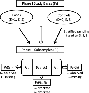
Figure 1: Data structure under two-phase sampling with partial missingness in phase II genetic covariates from the Molecular Epidemiology of Colorectal Cancer study.

The rest of the paper is organized as follows. In Section 2 we present the model ingredients: the likelihood, priors and posteriors. In Section 3 we discuss the analysis of statin x gene interaction in the MECC study. In Section LABEL:tpsim we conduct a simulation study to compare the various maximum likelihood and score based approaches with the Bayesian approach. Section LABEL:tpdiscuss concludes with a discussion.

2 Proposed methods

2.1 The likelihood

We refer to Figure 1 for understanding the data structure and construction of our likelihood. Let $u$ and $D$ denote the subject indicator and disease status, respectively. Here, $E$ is environmental exposure and $\mathbf{S}$ are basic demographic covariates as described before. Let $W=(E,\mathbf{S})$. There are $N$ individuals in phase I and $M$ individuals in phase II. To simplify notation, we write the retrospective likelihood corresponding to a two-gene model ($G_{1}$, $G_{2}$), with the understanding that the methods/notation can be directly extended to gene-sets ($\mathbf{G}_{1},\mathbf{G}_{2}$) where each contain multiple SNPs. The two-phase likelihood has the following form to capture the sampling phases and the missingness patterns in $\mathbf{G}$ (Figure 1):

$${\mathrm{L}}^{\mathrm{TP}} = \prod_{u\in P_{1}\setminus P_{2}}\mathrm{P}(W_{u}|D_{u})\times\prod_{u\in P_{2}(G_{1})}\mathrm{P}(G_{1u},W_{u}|D_{u})$$

$${}\times\prod_{u\in P_{2}(G_{2})}\mathrm{P}(G_{2u},W_{u}|D_{u})\times\prod_{u\in P_{2}(G_{1},G_{2})}\mathrm{P}(G_{1u},G_{2u},W_{u}|D_{u}).$$

Each term in ${\mathrm{L}}^{\mathrm{TP}}$ can be factorized by using $\mathrm{P}(G_{1},G_{2},W|D)=\{\mathrm{P}(D|G_{1},\break G_{2},W)$ $\mathrm{P}(G_{1},G_{2}|W)\mathrm{P}(W)\}/\mathrm{P}(D)$. This retrospective likelihood is then marginalized over the missing data in each term. We assume missing completely at random [LitRub02] for the genotype data collected at phase II. The likelihood is then expressed as

$$\qquad{\mathrm{L}}^{\mathrm{TP}} = \prod_{u\in P_{1}\setminus P_{2}}\sum_{g_{1},g_{2}}\mathrm{P}(D_{u}|g_{1},g_{2},W_{u}){\mathrm{P}(g_{1},g_{2}|W_{u})}\mathrm{P}(W_{u})/\mathrm{P}(D_{u})$$

$${}\times\prod_{u\in P_{2}(G_{1})}\sum_{g_{2}}\mathrm{P}(D_{u}|G_{1u},g_{2},W_{u}){\mathrm{P}(G_{1u},g_{2}|W_{u})}\mathrm{P}(W_{u})/\mathrm{P}(D_{u})$$

$${}\times\prod_{u\in P_{2}(G_{2})}\sum_{g_{1}}\mathrm{P}(D_{u}|g_{1},G_{2u},W_{u}){\mathrm{P}(g_{1},G_{2u}|W_{u})}\mathrm{P}(W_{u})/\mathrm{P}(D_{u})$$

$${}\times\prod_{u\in P_{2}(G_{1},G_{2})}\mathrm{P}(D_{u}|G_{1u},G_{2u},W_{u}){\mathrm{P}(G_{1u},G_{2u}|W_{u})}\mathrm{P}(W_{u})/\mathrm{P}(D_{u}),$$

where $\mathrm{P}(D_{u})=\sum_{g_{1},g_{2}}\int_{w}\mathrm{P}(D_{u}|g_{1},g_{2},w)\mathrm{P}(g_{1},g_{2}|w)\mathrm{P}(dw)$ with the integral replaced by the sum when components of $W$ are discrete. Corresponding to this likelihood, there are three model ingredients:

1. A disease risk model. We assume $\mathrm{P}(D=1|G_{1}=g_{1},G_{2}=g_{2},W=w;\bolds{\beta})=H[\{\beta_{0}+m(g_{1},g_{2},w;\bolds{\beta})\}]$, where $H$ is the logistic function $H(u)=\{1+\exp(-u)\}^{-1}$. Typical choice of $m$ involves, say, for two genes $G_{1}$ and $G_{2}$, $m(g_{1},g_{2},w;\bolds{\beta})=\beta_{G_{1}}g_{1}+\beta_{G_{2}}g_{2}+\beta_{E}e+{\bolds{\beta}^{\top}_{S}}\mathbf{s}+\beta_{G_{1}G_{2}}g_{1}g_{2}+\beta_{G_{1}E}g_{1}e+\beta_{G_{2}E}g_{2}e$, noting that $w=(e,\mathbf{s})$.

2. A model for $(G_{1},G_{2}|W=(E,\mathbf{S}))$. For genotype data at a bi-allelic locus, $G_{j}$ can take three possible values (“$g_{0}=\mbox{aa}$,” “$g_{1}=\mbox{Aa}$” and “$g_{2}=\mbox{AA}$”). We assume, $\mathrm{P}(G_{1}=g_{j},G_{2}=g_{j}^{\prime}|W=w;\bolds{\lambda})=q_{jj^{\prime}}(w;\bolds{\lambda}),j,j^{\prime}=0,1,2$. This specification will require a joint model for multivariate categorical data (trinary for SNP data at a bi-allelic locus). Under gene–gene and gene-environment independence, the model can in general be factorized conditional on covariates $\mathbf{S}$, for $j,j^{\prime}=0,1,2$,

$$\underbrace{\mathrm{P}\bigl{(}G_{1}=g_{j},G_{2}=g_{j}^{\prime}|E=e,\mathbf{S}=\mathbf{s};\bolds{\lambda}\bigr{)}=\mathrm{P}(G_{1}=g_{j}|\mathbf{S}=\mathbf{s},\bolds{\lambda}_{1})\mathrm{P}\bigl{(}G_{2}=g_{j}^{\prime}|\mathbf{S}=\mathbf{s},\bolds{\lambda}_{2}\bigr{)}}_{\mathrm{under}\ \mathrm{G}\mbox{-}\mathrm{G}\ \mathrm{and}\ \mathrm{G}\mbox{-}\mathrm{E}\ \mathrm{independence}}.$$

Instead of the above fully nonparametric model, we explore a parametric model for the joint distribution $\mathrm{P}(\mathbf{G}_{1},\mathbf{G}_{2}|W)$. We consider a class of log-linear models with linear by linear structure [Agr02] for parsimonious modeling of the $(G_{1},G_{2}|W)$ associations,

$$\log\bigl{\{}\mu\bigl{(}G_{1}=g_{j},G_{2}=g_{j}^{\prime}|E=e,\mathbf{S}=\mathbf{s};\bolds{\lambda}\bigr{)}\bigr{\}}$$

$$\qquad=\lambda_{0}+\lambda_{G_{1}}g_{j}+\lambda_{G_{2}}g_{j}^{\prime}+\lambda_{E}e+{\bolds{\lambda}^{\top}_{S}}\mathbf{s}$$ (2)

$$\qquad\quad{}+\lambda_{G_{1}G_{2}}g_{j}g_{j^{\prime}}+\lambda_{G_{1}E}g_{j}e+\lambda_{G_{2}E}g_{j^{\prime}}e+{\bolds{\lambda}^{\top}_{G_{1}S}}g_{j}\mathbf{s}+\bolds{\lambda}^{\top}_{G_{2}S}g_{j^{\prime}}\mathbf{s},$$

where $g_{j}$ are chosen ordinal scores, typically 0, 1, 2 [Agr02]. This is the common allelic dosage coding under a log-additive genetic susceptibility model. Our method could easily be extended to a co-dominant coding of the genetic factor using two dummy variables. Since log-additivity is often assumed for screening interactions, and for simplicity of presentation in terms of one parameter estimate as opposed to two, we proceed with this additive coding. Additionally, even if the true genetic susceptibility model is co-dominant with the disease-causing allele, for a tagging marker which is correlated to this causal allele, one would not a’priori know the direction of association of the marker allele and causal allele. PfeGai03 show that the additive scores are more robust to choice of marker allele and varying correlation scenarios. In case of high-dimensional $\mathbf{G}$, we can further reduce the dimensionality of the problem by assuming common association parameters $\lambda_{\mathit{GE}}$ and $\lambda_{\mathit{GS}}$ between similar functional groups of SNPs. As discussed in Agr02, this Poisson log-linear model has a corresponding multinomial representation. Thus, the probability of $P_{G_{1},G_{2}}({g_{j},g_{j}^{\prime}|\bolds{\lambda}})=P(G_{1}=g_{j},G_{2}=g_{j}^{\prime}|E=e,\mathbf{S}=\mathbf{s})$ can be written in terms of the multinomial probabilities,

$$P_{G_{1},G_{2}}\bigl{(}{g_{j},g_{j}^{\prime}|\bolds{\lambda}}\bigr{)}$$

$$\qquad=\exp\bigl{(}\lambda_{G_{1}}g_{j}+\lambda_{G_{2}}g_{j}^{\prime}+\lambda_{G_{1}G_{2}}g_{j}g_{j^{\prime}}$$

$$\qquad\quad\hskip 17.5pt{}+\lambda_{G_{1}E}g_{j}e+\lambda_{G_{2}E}g_{j}^{\prime}e+{\bolds{\lambda}^{\top}_{G_{1}S}}g_{j}\mathbf{s}+{\bolds{\lambda}^{\top}_{G_{2}S}}g_{j}^{\prime}\mathbf{s}\bigr{)}$$

$$\qquad\quad{}\times\Biggl{(}\sum_{l=0}^{2}\sum_{l^{\prime}=0}^{2}\exp\bigl{(}\lambda_{G_{1}}g_{l}+\lambda_{G_{2}}g_{l}^{\prime}+\lambda_{G_{1}G_{2}}g_{l}g^{\prime}_{l^{\prime}}$$

$$\qquad\quad\hskip 71.0pt{}+\lambda_{G_{1}E}g_{l}e+\lambda_{G_{2}E}g^{\prime}_{l^{\prime}}e+{\bolds{\lambda}^{\top}_{G_{1}S}}g_{l}\mathbf{s}+{\bolds{\lambda}^{\top}_{G_{2}S}}g^{\prime}_{l^{\prime}}\mathbf{s}\bigr{)}\Biggr{)}^{-1}.$$

Note that gene–gene and gene-environment independence in the above model (2.1) will imply $\lambda_{G_{1}E}\equiv\lambda_{G_{2}E}\equiv\lambda_{G_{1}G_{2}}\equiv 0$.

3. A model for $W=(E,\mathbf{S})$. A nonparametric and flexible model for the distribution of $W$ is desired. Recall that $W$ can be a mixed set of quantitative and categorical variables. For the MECC example $W$ is a set of categorical covariates, which will be our primary focus in this paper. The approach for modeling the joint distribution of a set of categorical variables that we follow for $W$ can also be applied to the the joint distribution of the trinary genotype variables $\mathbf{G}_{1}$ and $\mathbf{G}_{2}$ in (2.1) as well. However, reflecting prior faith on the gene–gene and gene-environment independence assumptions through direct priors on parameters $\lambda_{G_{1}E},\lambda_{G_{2}E},\lambda_{G_{1}G_{2}}$ in the log-linear model is more straightforward for a practitioner (2.1). This is the primary reason for using (2.1) for the second component $P(G_{1},G_{2}|W=(E,\mathbf{S}))$.

Let $\mathbf{W}_{u}=(E_{u},\mathbf{S}_{u})$ denote the $W$ data corresponding to subject $u$, $u=1,\ldots,N$. Here $W_{u}$ is $p\times 1$ vector of $p$ categorical variables, that is, $W_{u}=(w_{u1},\ldots,w_{up})$ for a subject $u$. Assume that the $j$th component of $W$ can have $d_{j}$ values $j=1,\ldots,p$. In order to parsimoniously model this $(d_{1}\times d_{2}\times\cdots\times d_{p})$ joint distribution, DX first note that the joint distribution of two categorical variables can always be expressed as a finite mixture of product-multinomial distributions. Extending this idea, DX introduce a latent class index variable $z_{u}\in\{1,\ldots,k\}$, such that $w_{ur},w_{ut},r,t\in\{1,\ldots,p\},r\neq t$, are conditionally independent given $z_{u}$. Then the joint distribution for $\mathbf{w}_{u}$ has this finite mixture representation,

$$P_{W}(w_{u1}=c_{1},\ldots,w_{up}=c_{p})$$

$$\qquad=\sum_{h=1}^{k}P(w_{u1}=c_{1},\ldots,w_{up}=c_{p}|z_{u}=h)P(z_{u}=h)$$ (3)

$$\qquad=\sum_{h=1}^{k}P(z_{u}=h)\prod_{j=1}^{p}P(w_{uj}=c_{j}|z_{u}=h).$$

For notational convenience, we rewrite (2.1) as

$$P_{W}(w_{u1}=c_{1},\ldots,w_{up}=c_{p}) = \pi_{c_{1}\cdots c_{p}}=\sum_{h=1}^{k}\nu_{h}\prod_{j=1}^{p}\psi_{hc_{j}}^{(j)},$$

$$\sum_{c_{1}=1}^{d_{1}}\cdots\sum_{c_{p}=1}^{d_{p}}\pi_{c_{1}\cdots c_{p}} = 1,$$

where $\bolds{\nu}=(\nu_{1},\ldots,\nu_{k})^{\top}$ is a probability vector with $\nu_{h}=P(z_{u}=h)$ and $\psi_{hc_{j}}^{(j)}=P(w_{uj}=c_{j}|z_{u}=h)$ is a $d_{j}\times 1$ probability vector, that is, the conditional probability of $w_{uj}=c_{j}$, given that subject $u$ is in latent class $h$ for $j=1,\ldots,p$. We will discuss the choice of $k$ through a Dirichlet process prior structure on this latent class probability model in the next section.

Remark 1.

While ChaChe07 and ChaCar05 use profile likelihood for handling the distribution of $W$ nonparametrically, it has been a challenging task in the Bayesian framework to posit a flexible model for $\mathbf{W}=(E,\mathbf{S})$ which could be a mixture of categorical and continuous covariates. In this mixed case, Muletal99 model the joint distribution of the continuous covariates through a Dirichlet process mixture of normals. Then, conditional on the continuous covariates, the categorical variables have a joint multivariate probit distribution. A recent paper by BhaDun extends the above DX construction for categorical data to handle joint distribution modeling of more complex data, including continuous and discrete data. They extend the conditional independence idea and replace the product-multinomial structure in (2.1) by a product of various kernels, such as Gaussian, Poisson and more complex univariate or multivariate distributional kernels. The MECC example does not require going beyond the original DX construction, but with continuous $E$, this is what we would adopt.

Remark 2.

If the phase I sample is a cohort study, with disease endpoint $D$, then the corresponding likelihood is proportional to

$$\mathrm{L}^{\mathrm{cohort},\mathrm{TP}} \propto \prod_{u\in P_{1}\setminus P_{2}}\sum_{g_{1},g_{2}}\mathrm{P}(D_{u}|g_{1},g_{2},W_{u}){\mathrm{P}(g_{1},g_{2}|W_{u})}$$

$${}\times\prod_{u\in P_{2}(G_{1})}\sum_{g_{2}}\mathrm{P}(D_{u}|G_{1u},g_{2},W_{u}){\mathrm{P}(G_{1u},g_{2}|W_{u})}$$

$${}\times\prod_{u\in P_{2}(G_{2})}\sum_{g_{1}}\mathrm{P}(D_{u}|g_{1},G_{2u},W_{u}){\mathrm{P}(g_{1},G_{2u}|W_{u})}$$

$${}\times\prod_{u\in P_{2}(G_{1},G_{2})}\mathrm{P}(D_{u}|G_{1u},G_{2u},W_{u}){\mathrm{P}(G_{1u},G_{2u}|W_{u})}.$$

Similarly, if environmental data $E$ is collected in phase II as well, the first term representing the phase I cohort likelihood can also involve an integral over the missing $E$ data with respect to a probability distribution $dF(E)$, exactly as in equation (3) of ChaChe07. A surrogate measure of $E$, namely, $E^{*}$, may be available in phase I and a measurement error model relating $E$ and $E^{*}$ can also be used to construct a joint likelihood of phases I and II data.

2.2 Priors

As mentioned before, for this complex retrospective likelihood formulation, we have three sets of parameters from the above three ingredients of the likelihood. For $\bolds{\beta}$ in the disease risk model, we use a spike and slab type mixture prior to handle variable selection in a high-dimensional disease risk model with multiple markers. For $\bolds{\lambda}$ in the multivariate gene model, the Bayesian hierarchical approach provides a flexible way to allow for uncertainty around the assumption of gene–gene and gene-environment independence, through prior on $\lambda_{G_{1}G_{2}},\lambda_{G_{1}E}$ and $\lambda_{G_{2}E}$. When sparsity occurs in a certain configuration of $(\mathbf{G}_{1},\mathbf{G}_{2},\mathbf{W})$ or dimension of $(\mathbf{G}_{1},\mathbf{G}_{2},\mathbf{W})$ grows, the frequentist profile likelihood estimation may become unstable and the log-linear model with shared parameters across gene-sets and the DX latent mixture construction aid with such situations. We follow the same sequence as in the previous section to describe the prior structure on the parameters.

1. In the presence of multiple genes in $\mathbf{G}_{1}$ and $\mathbf{G}_{2}$, the logistic disease risk model can potentially have many pairwise and higher order interaction terms. We implement a scalable variable selection framework via spike and slab type priors [MitBea88, GeoMcc93] on the parameters $\bolds{\beta}$ in the disease risk model $P(D|\mathbf{G}_{1},\mathbf{G}_{2},W;\bolds{\beta})$. We impose mixture prior distributions on each component of $\bolds{\beta}$, say, $(\beta_{0},\beta_{G_{1}},\break\beta_{G_{2}},\beta_{E},\beta_{S},\beta_{G_{1}G_{2}},\beta_{G_{1}E}$, $\beta_{G_{2}E})$ for a two-gene model. In general, we denote this vector by $\bolds{\beta}_{n_{\beta}\times 1}=\{\beta_{r},r=1,\ldots,n_{\beta}\}$. Given a latent variable $p_{0}$ representing the mixture weight on the “not informative” regression coefficients, we describe the hierarchical prior structure as follows:

$$\beta_{r}|f_{r},{\tau}_{r} \stackrel{{\scriptstyle\mathrm{ind}}}{{\sim}} N\bigl{(}0,f_{r}\tau_{r}^{2}\bigr{)},\qquad r=1,\ldots,n_{\beta},$$

$$f_{r}|v_{0},p_{0} \stackrel{{\scriptstyle\mathrm{i.i.d.}}}{{\sim}} p_{0}\delta_{v_{0}}(\cdot)+(1-p_{0})\delta_{1}(\cdot),$$

$$\tau_{r}^{-2}|a_{1},a_{2} \stackrel{{\scriptstyle\mathrm{i.i.d.}}}{{\sim}} \operatorname{Gamma}(a_{1},a_{2}),$$

$$p_{0} \stackrel{{\scriptstyle\mathrm{i.i.d.}}}{{\sim}} \operatorname{Beta}(a,b).$$

As discussed in IshRao03, $v_{0}$ in the above specification is assumed to be a small positive value near 0. Note that $f_{r}$ can assume two values $v_{0}$ or 1. At each iteration of posterior sampling, $f_{r}$ takes value $1$ if sampled $\beta_{r}$ is significantly away from zero, implying that the $r$th covariate is potentially informative. Note that a key feature of this prior specification is that the marginal prior variance of $\beta_{r}$ is calibrated as $\operatorname{var}(\beta_{r})=f_{r}\tau_{r}^{2}$ and has a bimodal distribution. Large $\operatorname{var}(\beta_{r})$ can occur when $f_{r}=1$ and $\tau_{r}^{2}$ is large, inducing large values of $\beta_{r}$, identifying potentially informative covariates. Small values of $\operatorname{var}(\beta_{r})$ occur when $f_{r}$ assumes value $v_{0}$, leading to values of $\beta_{r}$ that are near zero, suggesting that $\beta_{r}$ is potentially uninformative. The value of $p_{0}$ controls how likely it is for $f_{r}$ to be $v_{0}$ or $1$, thus controlling how many $\beta_{r}$ are nonzero or the complexity of the model. The Gamma parameters $(a,b)$ control the degree of parsimony through the prior on $p_{0}$. We set $(a,b)=(1,1)$, that is, a uniform prior on $p_{0}$, for the analysis we present in the main text. Note that $(a_{1},a_{2})$ determines the prior on $\tau_{r}^{2}$ and thus the variance of $\beta_{r}$. We fix $(a_{1},a_{2})$ at $(5,50)$ to allow the possibility of large prior variances on $\beta$. The values used for the hyperparameters in the hierarchy are exactly as recommended in IshRao03.

2. In the joint log-linear model (2.1), we typically assume vague normal priors with large variance on the parameters $(\lambda_{G_{1}},\lambda_{G_{2}},\lambda_{G_{1}S}$, $\lambda_{G_{2}S})$. In our data example, we have used a $N(0,10^{4})$ prior. On the other hand, for the $G$-$E$ pairwise association parameters $(\lambda_{G_{1}G_{2}},\lambda_{G_{1}E},\lambda_{G_{2}E})$, we reflect a priori information on $G$-$G$ or $G$-$E$ independence via a normal prior centered at zero but with two different choices for the prior variance. In the first set of priors we reflect the belief that with 95% probability the association parameter lies between $\log(0.8)$ and $\log(1.2)$. This leads to an approximate $\mbox{SD}=0.1$ under a normal distribution and, thus, we assume an informative prior of $N(0,10^{-2})$. In the second choice, following the empirical Bayes estimation of MukCha08, we compute association parameters for $G_{1}$-$G_{2}$, $G_{1}$-$E$, and $G_{2}$-$E$ in the control subjects in the data, say, $\hat{\theta}$, and use a data-driven prior $N(0,{\hat{\theta}^{2}})$ on $\lambda_{G_{1}G_{2}}$, $\lambda_{G_{1}E}$ and $\lambda_{G_{2}E}$.

3. The mixture representation in (2.1) requires determining the number of latent classes $k$. Following DX, instead of selecting a fixed $k$, a Bayesian nonparametric approach is carried out through the Dirichlet process prior specification on $\bolds{\nu}$:

$$\bolds{\pi} = \sum_{h=1}^{\infty}\nu_{h}\bolds{\psi}_{h},\qquad\bolds{\psi}_{h}=\bolds{\psi}_{h}^{(1)}\otimes\cdots\otimes\bolds{\psi}_{h}^{(p)},\qquad h=1,\ldots,\infty,$$

$$\bolds{\psi}_{h}^{(j)} \sim \operatorname{Dirichlet}(a_{j1},\ldots,a_{jd_{j}})\qquad\mbox{independently for }j=1,\ldots,p,$$

$$\nu_{h} = \sum_{h=1}^{\infty}V_{h}\prod_{l<h}(1-V_{l}),\qquad V_{h}\sim\operatorname{Beta}(1,\alpha),$$

$$\alpha \sim \operatorname{Gamma}(a_{\alpha},b_{\alpha}),$$

where $\otimes$ is the outer product. The parameter $\alpha$ is a hyper-parameter that controls the rate of decrease from the stick-breaking process [Set94]. For example, in the case of small values of $\alpha$, $\nu_{h}$ decreases toward zero quickly with increasing $h$, thus putting most of the weight on the first few components, leading to a sparse representation. The hyperprior on $\alpha$ allows one to data-adaptively determine the degree of sparseness or the number of components needed. As discussed in DunXin09, we set $(a_{\alpha},b_{\alpha})=(1/4,1/4)$ for a vague prior which implies the probability of independence across components of $w$ in the product multinomial model to be $0.5$. We set uniform priors for each category probability $\bolds{\psi}$ with $a_{j1}=\cdots=a_{jd_{j}}=1$, for $j=1,\ldots,p$ and let the data dominate over priors. To minimize large numbers of mixture components instead of using infinite mixtures, we truncate the maximum of the number of mixture components $k$ at $30$ in the real data example [Ahnetal]. We study sensitivity with respect to this truncation threshold in Table 1.

2.3 Posterior sampling

In the full likelihood (2.1), we would like to point out that the three components are linked with each other through the sum over each component in the expression for $P(D)$ in the denominator. We denote the two-phase likelihood in (2.1) by $\mathrm{L}_{\mathrm{TP}}$ which involves the parameters $(\bolds{\beta},\bolds{\lambda},\bolds{\psi},\mathbf{V},\alpha)$. The full conditionals are not reducible to a simpler closed form and are best represented by the following proportionality relations:

$$\beta_{r}|\cdot \propto {\mathrm{L}}^{\mathrm{TP}}\times\exp\biggl{(}-\frac{\beta_{r}^{2}}{2f_{r}\tau_{r}^{2}}\biggr{)},\qquad r=1,\ldots,n_{\beta},$$

$$\tau_{r}^{-2}|\cdot \propto \operatorname{Gamma}\biggl{(}a_{1}+0.5,a_{2}+\frac{\beta_{r}^{2}}{2f_{r}}\biggr{)},$$

$$f_{r}|\cdot \propto \bigl{\{}I(f_{r}=v_{0})p_{0}+I(f_{r}=1)(1-p_{0})\bigr{\}}\times\exp\biggl{(}-\frac{1}{2f_{r}\tau_{r}^{2}}\beta_{r}^{2}\biggr{)}\times f_{r}^{-0.5},$$

$$p_{0}|\cdot \propto \operatorname{Beta}\Biggl{(}a+\sum_{r=1}^{n_{\beta}}I(f_{r}=v_{0}),b+\sum_{r=1}^{n_{\beta}}I(f_{r}=1)\Biggr{)},$$

$$\lambda_{l}|\cdot \propto {\mathrm{L}}^{\mathrm{TP}}\times\exp\biggl{(}-\frac{\lambda_{l}^{2}}{2\sigma^{2}}\biggr{)},\qquad l=1,\ldots,n_{\lambda},$$

where $n_{\beta}$ and $n_{\lambda}$ again represent the number of parameters in $(\bolds{\beta},\bolds{\lambda})$, respectively.

Posterior sampling corresponding to $P(\mathbf{W})$: Let us recapitulate the model structure for $\mathbf{W}$ which is essentially a Dirichlet process mixture of discrete Dirichlet kernels. For $u=1,\ldots,N$ and $j=1,\ldots,p$,

$$w_{uj} \sim \operatorname{Multinomial}\bigl{(}\{1,\ldots,d_{j}\},\psi^{j}_{z_{u},1},\ldots,\psi^{j}_{z_{u},d_{j}}\bigr{)},$$

$$z_{u} \sim V_{h}\prod_{l<h}(1-V_{l})\delta_{h},\qquad V_{h}\sim\operatorname{Beta}(1,\alpha),\qquad\alpha\sim\operatorname{Gamma}(a_{\alpha},b_{\alpha}).$$

DX present an efficient data-augmented Gibbs sampling algorithm by augmenting the likelihood with latent constructs following Wal07. The details of the updating steps are described in the supplemental article [Ahnetal].

Note that while the entire likelihood in DX is constituted of $W$ data only, in our problem, $P(\mathbf{W})$ is embedded as a component in the joint retrospective likelihood ${\mathrm{L}}^{\mathrm{TP}}$ in (2.1). Thus, for updating the parameters involved in $\mathrm{P}(\mathbf{W})$, say, $\bolds{\theta}(\mbox{$=$}\{\bolds{\psi},\mathbf{V},\alpha\})$, we use the Metropolis Hastings algorithm. Only the terms $\prod_{u}\mathrm{P}(\mathbf{W}_{u})/\mathrm{P}(D_{u})$ from the full likelihood (2.1) involve $\bolds{\theta}$, where $\mathrm{P}(D_{u})=\sum_{g_{1},g_{2}}\sum_{\mathbf{w}}\mathrm{P}(D_{u}|g_{1},g_{2},\mathbf{w})$ $\mathrm{P}(g_{1},g_{2}|\mathbf{w})\mathrm{P}(\mathbf{w})$. We draw $\bolds{\theta}$ following the DX algorithm and for the proposal density of $\bolds{\theta}$ we consider the implied full conditional $q(\bolds{\theta}^{\mathrm{new}}|\mathbf{W})$ as determined by this algorithm. Then given $\bolds{\lambda},\bolds{\beta}$, we repeat the following updates of $\bolds{\theta}$:

• At iteration $l$, sample a vector $\bolds{\theta}^{\mathrm{new}}$ from $q(\bolds{\theta}^{\mathrm{new}}|\mathbf{W})$ as described in the DunXin09 algorithm.

• Compute the acceptance ratio

  $$r\bigl{(}\bolds{\theta}^{\mathrm{new}},\bolds{\theta}_{l}\bigr{)}=\operatorname{min}\biggl{[}1,\frac{\prod_{u}\mathrm{P}(D_{u}|\bolds{\theta}_{l},\bolds{\lambda},\bolds{\beta})}{\prod_{u}\mathrm{P}(D_{u}|\bolds{\theta}^{\mathrm{new}},\bolds{\lambda},\bolds{\beta})}\biggr{]}.$$

  In calculating the acceptance ratio, we note that the numerator and denominator $\prod_{u}\{\mathrm{P}(W_{u}|\bolds{\theta}^{\mathrm{new}})\}p(\bolds{\theta}^{\mathrm{new}})$ $q(\bolds{\theta}_{l}|\mathbf{W})/\prod_{u}\{\mathrm{P}(W_{u}|\bolds{\theta}_{l})\}p(\bolds{\theta}_{l})q(\bolds{\theta}^{\mathrm{new}}|\break\mathbf{W})$ are canceled out where $p(\bolds{\theta})$ is a prior for $\bolds{\theta}$.

• If $r(\bolds{\theta}^{\mathrm{new}},\bolds{\theta}_{l})<U$ where $U\sim\operatorname{unif}(0,1)$, we set $\bolds{\theta}_{l+1}=\bolds{\theta}^{\mathrm{new}}$. Otherwise, the candidate vector $\theta^{\mathrm{new}}$ is rejected and $\bolds{\theta}_{l+1}=\bolds{\theta}_{l}$.

• Repeat the steps until the posterior chains converge.

Given the full conditionals, we implement the Gibbs sampler [GemGem84] with Metropolis Hastings updates to sample from respective full conditional distributions. For each parameter, we iterate 50,000 times and discard the first 40,000 iterations as “burn-in.” We check convergence of the chains using trace plots and the numerical diagnostic statistic “potential scale reduction factor” [Dav92] using the R package CODA [Pluetal]. Auto and cross-correlation checks are performed and a thinning of every tenth observation is carried out. Remaining posterior samples are used to construct estimated posterior summaries needed for Bayesian inference.

3 The Molecular Epidemiology of Colorectal Cancer study

In this section we describe the motivating example from the MECC study in detail and present analysis results. We use data on 1746 cases and 1853 controls with completely observed response to the question whether statins were used for more than 5 years. The binary variable “statin use of at least 5 years” ($E$) is the environmental factor of interest with 91% “NO” and 9% “YES.”

We adjust for completely observed confounders and precision variables ($\mathbf{S}$): age ($S_{1}$), gender ($S_{2}$), ethnicity ($S_{3}$), physical activity ($S_{4}$), family history of CRC ($S_{5}$), vegetable consumption ($S_{6}$), NSAID usage within 3 year ($S_{7}$) and Aspirin usage within 3 year ($S_{8}$). Age and ethnicity variables were dichotomized as Age $\geq$ or $<$ 50 (94% and 6%, resp.), and “Ashkenazi” and “Non-Ashkenazi” (68% and 32%, resp.). Gender $(S_{3})$ was coded as 1 (50%) for male and 0 (50%) for female. The remaining binary factors $(S_{4},S_{5},S_{6},S_{7},S_{8})$ are classified to 1 or “YES” with the proportions of (0.36, 0.09, 0.31, 0.02, 0.20), respectively.

For genotyping at phase II, stratified-sampling based on the disease status ($D$) and statin use ($E$) was carried out. All case-control subjects with statin use (“YES”) were included at the phase II sample. We have 1200 cases and 1200 controls at phase II with data available on 294 trinary SNPs $\mathbf{G}=(G_{1},\ldots,G_{294})$. Genotype data are not completely observed even at phase II due to technical genotyping failures for a limited number of SNPs. Among 2400 case-control subjects at phase II, 56 subjects and 20 had partial genotype information on two subsets of SNPs. We did not have a dense set of markers typed across the genome to successfully impute these missing genotypes, thus we consider a marginalized likelihood as in (2.1).

Among 294 SNPs, we first illustrate our methods with two SNPs on two genes, $RS1800775$ on CETP ($G_{1}$) and $RS1056836$ on CYP1B1 ($G_{2}$), where both SNPs exhibit significant interactions with statin use in an initial single marker interaction analysis. We compare our methods for this simple two SNP model to some of the alternative methods that can only handle single marker interaction analysis. The raw frequencies of the cross-classification of case-control status ($D$), statins ($E$), genotypes $G_{1}$ and $G_{2}$ are shown in online supplementary Table 1 [Ahnetal]. Simple logistic regression analysis was carried out to examine $G_{1}$-$E$ and $G_{2}$-$E$ association among control subjects and yielded odds ratios of 1.11 and 1.01 and corresponding p-values of 0.30 and 0.91, respectively. Based on a chi-squared test for independence, $G_{1}$-$G_{2}$ reveals no association (p-value of 0.90) These tests suggest that the data support $G_{1}$-$E$, $G_{2}$-$E$ and $G_{1}$-$G_{2}$ independence assumption.

= (a) Analysis results for the MECC study data with statins ($E$), $G_{1}$ $RS1800775$ on CETP and $G_{2}$ $RS1056836$ on CYP1B1. The model adjusts age ($S_{1}$, $\mbox{``$>$50''}=1$, $\mbox{``$\leq$50''}=0$), gender ($S_{2}$, $\mbox{male}=1$, $\mbox{female}=0$), ethnicity ($S_{3}$, $\mbox{Ashkenazi}=1$, $\mbox{Non-Ashkenazi}=0$), sports activity ($S_{4}$, $\mbox{Yes}=1$, $\mbox{No}=0$), vegetable consumption ($S_{5}$, $\mbox{High}=1$, $\mbox{Low}=0$), family history of CRC ($S_{6}$, $\mbox{Yes}=1$, $\mbox{No}=0$), the use or nonuse of NSAID within 3 years ($S_{7}$, $\mbox{Yes}=1$, $\mbox{No}=0$), the use or nonuse of Aspirin within 3 years ($S_{8}$, $\mbox{Yes}=1$, $\mbox{No}=0$). Under the TPFB method the “est.” corresponds to the posterior mean, whereas PSD corresponds to posterior standard deviation. The methods that yield the smallest PSD are in bold font in each row TPFB TPFB$\bolds{{}_{\mathrm{emp}}}$ WL PL UML CML EB est.(PSD) est.(PSD) est.(se) est.(se) est.(se) est.(se) est.(se) Exposure variables    $G_{1}$ $0.04\mbox{ }(0.09)$ $0.01\mbox{ }(0.09)$ $0.00\mbox{ }(0.09)$ $0.00\mbox{ }(0.09)$ $0.00\mbox{ }(0.09)$ $\mbox{{0.00}}\mbox{ }\mbox{{(0.08)}}$ $\mbox{{$\bolds{-}$0.07}}\mbox{ }\mbox{{(0.08)}}$    $G_{2}$ $-0.04\mbox{ }(0.10)$ $-0.06\mbox{ }(0.10)$ $-0.13\mbox{ }(0.10)$ $-0.13\mbox{ }(0.10)$ $-0.13\mbox{ }(0.10)$ $\mbox{{$\bolds{-}$0.12}}\mbox{ }\mbox{{(0.08)}}$ $\mbox{{$\bolds{-}$0.12}}\mbox{ }\mbox{{(0.08)}}$    Statin use ${-1.29}\mbox{ }(0.30)$ $\mbox{{$\bolds{-}$1.32}}\mbox{ }\mbox{{(0.27)}}$ ${-1.30}\mbox{ }(0.30)$ $-1.30\mbox{ }(0.30)$ $-1.40\mbox{ }(0.30)$ $-1.54\mbox{ }(0.28)$ $-1.51\mbox{ }(0.29)$    $G_{1}$ x $G_{2}$ $0.01\mbox{ }(0.07)$ $\mbox{{0.03}}\mbox{ }\mbox{{(0.05)}}$ $0.05\mbox{ }(0.08)$ $0.06\mbox{ }(0.08)$ $0.06\mbox{ }(0.08)$ $0.06\mbox{ }(0.06)$ $0.06\mbox{ }(0.06)$    $G_{1}$ x statin use $0.34\mbox{ }({0.17})$ $\mbox{{0.34}}\mbox{ }\mbox{{({0.15})}}$ $0.25\mbox{ }(0.18)$ $0.25\mbox{ }(0.18)$ $0.25\mbox{ }(0.18)$ $\mbox{{0.38}}\mbox{ }\mbox{{({0.15})}}$ $0.34\mbox{ }(0.17)$    $G_{2}$ x statin use $\mbox{{0.33}}\mbox{ }\mbox{{(0.16)}}$ $\mbox{{0.33}}\mbox{ }\mbox{{({0.16})}}$ $0.38\mbox{ }(0.18)$ $0.38\mbox{ }(0.19)$ $0.38\mbox{ }(0.20)$ $0.38\mbox{ }(0.18)$ $0.38\mbox{ }(0.19)$ Gene-statin and gene–gene association parameters from $P(G_{1},G_{2}|E,\mathbf{S})$    $\lambda_{G_{1}G_{2}}$ $0.02\mbox{ }(0.05)$ $0.00\mbox{ }(0.05)$    $\lambda_{G_{1}E}$ $0.05\mbox{ }(0.07)$ $0.08\mbox{ }(0.06)$    $\lambda_{G_{2}E}$ $0.01\mbox{ }(0.07)$ $0.01\mbox{ }(0.07)$ (b) Sensitivity analysis with respect to the maximum number of allowable mixture components $k_{\mathrm{max}}$, and the prior on $G$-$G$ and $G$-$E$ association parameters $\bolds{\lambda}$ $\bolds{G_{1}}$ $\bolds{G_{2}}$ Statin use $\bolds{G_{1}}$ x $\bolds{G_{2}}$ $\bolds{G_{1}}$ x statin use $\bolds{G_{2}}$ x statin use $k_{\mathrm{max}}=10$ TPFB 0.05 (0.10) $-$0.03 (0.10) $-$1.29 (0.30) 0.01 (0.07) 0.36 (0.16) 0.32 (0.17) TPFB${}_{\mathrm{emp}}$ 0.01 (0.09) $-$0.06 (0.10) $-$1.32 (0.29) 0.03 (0.07) 0.31 (0.15) 0.32 (0.16) $k_{\mathrm{max}}=30$ TPFB${}_{\mathrm{non}}$ 0.05 (0.11) $-$0.03 (0.11) $-$1.29 (0.31) 0.01 (0.07) 0.34 (0.19) 0.34 (0.21) []TPFB,TPFBemp,TPFBnon:Two-phasefullBayes[withinformative

Table 1: