Estimating treatment effect heterogeneity in randomized program evaluation

Abstract

When evaluating the efficacy of social programs and medical treatments using randomized experiments, the estimated overall average causal effect alone is often of limited value and the researchers must investigate when the treatments do and do not work. Indeed, the estimation of treatment effect heterogeneity plays an essential role in (1) selecting the most effective treatment from a large number of available treatments, (2) ascertaining subpopulations for which a treatment is effective or harmful, (3) designing individualized optimal treatment regimes, (4) testing for the existence or lack of heterogeneous treatment effects, and (5) generalizing causal effect estimates obtained from an experimental sample to a target population. In this paper, we formulate the estimation of heterogeneous treatment effects as a variable selection problem. We propose a method that adapts the Support Vector Machine classifier by placing separate sparsity constraints over the pre-treatment parameters and causal heterogeneity parameters of interest. The proposed method is motivated by and applied to two well-known randomized evaluation studies in the social sciences. Our method selects the most effective voter mobilization strategies from a large number of alternative strategies, and it also identifies the characteristics of workers who greatly benefit from (or are negatively affected by) a job training program. In our simulation studies, we find that the proposed method often outperforms some commonly used alternatives.

abstractwidth290pt

T1Supported by NSF Grant SES–0752050. The proposed methods can be implemented via open-source software FindIt [Ratkovic and Imai (2012)], which is freely available at the Comprehensive R Archive Network (http://cran.r-project.org/package=FindIt). This software also contains the results of our empirical analysis.

and

1 Introduction and motivating applications

While the average treatment effect can be easily estimated without bias in randomized experiments, treatment effect heterogeneity plays an essential role in evaluating the efficacy of social programs and medical treatments. We define treatment effect heterogeneity as the degree to which different treatments have differential causal effects on each unit. For example, ascertaining subpopulations for which a treatment is most beneficial (or harmful) is an important goal of many clinical trials. However, the most commonly used method, subgroup analysis, is often inappropriate and remains one of the most debated practices in the medical research community [e.g., Rothwell (2005), Lagakos (2006)]. Estimation of treatment effect heterogeneity is also important when (1) selecting the most effective treatment among a large number of available treatments, (2) designing optimal treatment regimes for each individual or a group of individuals [e.g., Manski (2004), Pineau et al. (2007), Moodie, Platt and Kramer (2009), Imai and Strauss (2011), Cai et al. (2011), Gunter, Zhu and Murphy (2011), Qian and Murphy (2011)], (3) testing the existence or lack of heterogeneous treatment effects [e.g., Gail and Simon (1985), Davison (1992), Crump et al. (2008)], and (4) generalizing causal effect estimates obtained from an experimental sample to a target population [e.g., Frangakis (2009), Cole and Stuart (2010), Hartman, Grieve and Sekhon (2010), Green and Kern (2010b), Stuart et al. (2011)]. In all of these cases, the researchers must infer how treatment effects vary across individual units and/or how causal effects differ across various treatments.

Two well-known randomized evaluation studies in the social sciences serve as the motivating applications of this paper. Earlier analyses of these data sets focused upon the estimation of the overall average treatment effects and did not systematically explore treatment effect heterogeneity. First, we analyze the get-out-the-vote (GOTV) field experiment where many different mobilization techniques were randomly administered to registered New Haven voters in the 1998 election [Gerber and Green (2000)]. The original experiment used an incomplete, unbalanced factorial design, with the following four factors: a personal visit, 7 possible phone messages, 0 to 3 mailings, and one of three appeals applied to visit and mailings (civic duty, neighborhood solidarity, or a close election). The voters in the control group did not receive any of these GOTV messages. Additional information on each voter includes age, residence ward, whether registered for a majority party, and whether the voter abstained or did not vote in the 1996 election. Here, our goal is to identify a set of GOTV mobilization strategies that can best increase turnout. Given the design, there exist 193 unique treatment combinations, and the number of observations assigned to each treatment combination ranges dramatically, from the minimum of 4 observations (visited in person, neighbor/civic-neighbor phone appeal, two mailings, with a civic appeal) to the maximum of $2956$ (being visited in person, with any appeal). The methodological challenge is to extract useful information from such sparse data.

The second application is the evaluation of the national supported work (NSW) program, which was conducted from 1975 to 1978 over 15 sites in the United States. Disadvantaged workers who qualified for this job training program consisted of welfare recipients, ex-addicts, young school dropouts, and ex-offenders. We consider the binary outcome indicating whether the earnings increased after the job training program (measured in 1978) compared to the earnings before the program (measured in 1975). The pre-treatment covariates include the 1975 earnings, age, years of education, race, marriage status, whether a worker has a college degree, and whether the worker was unemployed before the program (measured in 1975). Our analysis considers two aspects of treatment effect heterogeneity. First, we seek to identify the groups of workers for whom the training program is beneficial. The program was administered to the heterogeneous group of workers and, hence, it is of interest to investigate whether the treatment effect varies as a function of individual characteristics. Second, we show how to generalize the results based on this experiment to a target population. Such an analysis is important for policy makers who wish to use experimental results to decide whether and how to implement this program in a target population.

To address these methodological challenges, we formulate the estimation of heterogeneous treatment effects as a variable selection problem [see also Gunter, Zhu and Murphy (2011), Imai and Strauss (2011)]. We propose the Squared Loss Support Vector Machine (L2-SVM) with separate LASSO constraints over the pre-treatment and causal heterogeneity parameters (Section 2). The use of two separate constraints ensures that variable selection is performed separately for variables representing alternative treatments (in the case of the GOTV experiment) and/or treatment-covariate interactions (in the case of the job training experiment). Not only do these variables differ qualitatively from others, they often have relatively weak predictive power. The proposed model avoids the ad-hoc variable selection of existing procedures by achieving optimal classification and variable selection in a single step [e.g., Gunter, Zhu and Murphy (2011), Imai and Strauss (2011)]. The model also directly incorporates sampling weights into the estimation procedure, which are useful when generalizing the causal effects estimates obtained from an experimental sample to a target population.

To fit the proposed model with multiple regularization constraints, we develop an estimation algorithm based on a generalized cross-validation (GCV) statistic. When the derivation of an optimal treatment regime rather than the description of treatment effect heterogeneity is of interest, we can replace the GCV statistic with the average effect size of the optimal treatment rule [Imai and Strauss (2011), Qian and Murphy (2011)]. The proposed methodology with the GCV statistic does not require cross-validation and hence is more computationally efficient than the commonly used methods for estimation of treatment effect heterogeneity such as Boosting [Freund and Schapire (1999), LeBlanc and Kooperberg (2010)], Bayesian additive regression trees (BART) [Chipman, George and McCulloch (2010), Green and Kern (2010a)], and other tree-based approaches [e.g., Su et al. (2009), Imai and Strauss (2011), Lipkovich et al. (2011), Loh et al. (2012), Kang et al. (2012)]. While most similar to a Bayesian logistic regression with noninformative prior [Gelman et al. (2008)], the proposed method uses LASSO constraints to produce a parsimonious model.

To evaluate the empirical performance of the proposed method, we analyze the aforementioned two randomized evaluation studies (Section 3). We find that personal visits are uniformly more effective than any other treatment method, while sending three mailings with a civic duty message is the most effective treatment without a visit. In addition, every mobilization strategy with a phone call, but no personal visit, is estimated to have either a negative or negligible positive effect. For the job training study, we find that the program is most effective for low-education, high income Non-Hispanics, unemployed blacks with some college, and unemployed Hispanics with some high school. In contrast, the program would be least effective when administered to old, unemployed recipients, unmarried whites with a high school degree but no college, and high earning Hispanics with no college.

Finally, we conduct simulation studies to compare the performance of the proposed methodology with that of various alternative methods (Section 4). The proposed method admits the possibility of no treatment effect and yields a low false discovery rate, when compared to the nonsparse alternative methods that always estimate some effects. Despite reductions in false discovery, the method remains statistically powerful. We find that the proposed method has a comparable discovery rate and competitive predictive properties to these commonly used alternatives.

2 The proposed methodology

In this section we describe the proposed methodology by presenting the model and developing a computationally efficient estimation algorithm to fit the model.

2.1 The framework

We describe our method within the potential outcomes framework of causal inference. Consider a simple random sample of $N$ units from population $\mathcal{P}$, with a possibly different target population of inference $\mathcal{P}^{\ast}$. For example, the researchers and policy makers may wish to apply the GOTV mobilization strategies and the job training program to a population, of which the study sample is not representative. We consider a multi-valued treatment variable $T_{i}$, which takes one of $(K+1)$ values from $\mathcal{T}\equiv\{0,1,\ldots,K\}$ where $T_{i}=0$ means that unit $i$ is assigned to the control condition. In the GOTV study, we have a total of 193 treatment combinations ($K=193$), whereas the job training program corresponds to a binary treatment variable ($K=1$). The potential outcome under treatment $T_{i}=t$ is denoted by $Y_{i}(t)$, which has support $\mathcal{Y}$. Thus, the observed outcome is given by $Y_{i}=Y_{i}(T_{i})$ and we define the causal effect of treatment $t$ for unit $i$ as $Y_{i}(t)-Y_{i}(0)$.

Throughout, we assume that there is no interference among units, there is a unique version of each treatment, each unit has nonzero probability of assignment to each treatment level, and the treatment level is independent of the potential outcomes, possibly conditional on observed covariates [Rubin (1990), Rosenbaum and Rubin (1983)]. Such assumptions are met in randomized experiments, which are the focus of this paper. Under these assumptions, we can identify the average treatment effect (ATE) for each treatment $t$, $\tau(t)=\mathbb{E}(Y_{i}(t)-Y_{i}(0))$. In observational studies, additional difficulty arises due to the possible existence of unmeasured confounders.

One commonly encountered problem related to treatment effect heterogeneity requires selecting the most effective treatment from a large number of alternatives using the causal effect estimates from a finite sample. That is, we wish to identify the treatment condition $t$ such that $\tau(t)$ is the largest, that is, $t=\mathop{\arg\max}_{t^{\prime}\in\mathcal{T}}\tau(t^{\prime})$. We may also be interested in identifying a subset of the treatments whose ATEs are positive. When the number of treatments $K$ is large as in the GOTV study, a simple strategy of subsetting the data and conducting a separate analysis for each treatment suffers from the lack of power and multiple testing problems.

Another common challenge addressed in this paper is identifying groups of units for which a treatment is most beneficial (or most harmful), as in the job training program study. Often, the number of available pre-treatment covariates, $X_{i}\in\mathcal{X}$, is large, but the heterogeneous treatment effects can be characterized parsimoniously using a subset of these covariates, $\widetilde{X}_{i}\in\widetilde{\mathcal{X}}\subset\mathcal{X}$. This problem can be understood as identifying a sparse representation of the conditional average treatment effect (CATE), using only a subset of the covariates. We denote the CATE for a unit with covariate profile $\tilde{x}$ as $\tau(t;\tilde{x})=\mathbb{E}(Y_{i}(t)-Y_{i}(0)\mid\widetilde{X}_{i}=\tilde{x})$, which can be estimated as the difference in predicted values under $T_{i}=t$ and $T_{i}=0$ with $\widetilde{X}_{i}=\tilde{x}$. The sparsity in covariates greatly eases interpretation of this model.

We next turn to the description of the proposed model that combines optimal classification and variable selection to estimate treatment effect heterogeneity. For the remainder of the paper, we focus on the case of binary outcomes, that is, $\mathcal{Y}=\{0,1\}$. However, the proposed model and algorithm can be extended easily to nonbinary outcomes by modifying the loss function. We choose to model binary outcomes with the L2-SVM to illustrate our proposed methodology because it presents one of the most difficult cases for implementing two separate LASSO constraints. As we discuss below, our method can be simplified when the outcome is nonbinary (e.g., continuous, counts, multinomial, hazard) or the causal estimand of interest is characterized on a log-odds scale (with a logistic loss). In particular, readily available software can be adapted to handle these cases [Friedman, Hastie and Tibshirani (2010)].

2.2 The model

In modeling treatment effect heterogeneity, we transform the observed binary outcome to $Y_{i}^{\ast}=2Y_{i}-1\in\{\pm 1\}$. We then relate the estimated outcome $\widehat{Y}_{i}\in\{\pm 1\}$ and the estimated latent variable $\widehat{W}_{i}\in\Re$, as

$$\widehat{Y}_{i}=\operatorname{sgn}{(\widehat{W}_{i})}\qquad\mbox{where }\widehat{W}_{i}=\hat{\mu}+\hat{\beta}^{\top}Z_{i}+\hat{\gamma}^{\top}V_{i},$$

$Z_{i}$ is an $L_{Z}$ dimensional vector of treatment effect heterogeneity variables, and $V_{i}$ is an $L_{V}$ dimensional vector containing the remaining covariates. For example, when identifying the most efficacious treatment condition among many alternative treatments, $Z_{i}$ would consist of $K$ indicator variables (e.g., different combinations of mobilization strategies), each of which is representing a different treatment condition. In contrast, $V_{i}$ would include pre-treatment variables to be adjusted (e.g., age, party registration, turnout history). Similarly, when identifying groups of units most helped (or harmed) by a treatment, $Z_{i}$ would include variables representing interactions between the treatment variable (e.g., the job training program) and the pre-treatment covariates of interest (e.g., age, education, race, prior employment status and earnings). In this case, $V_{i}$ would include all the main effects of the pre-treatment covariates. Thus, we separate the causal heterogeneity variables of interest from the rest of the variables. We do not impose any restriction between main and interaction effects because some covariates may not predict the baseline outcome but do predict treatment effect heterogeneity. Finally, we choose the linear model because it allows for easy interpretation of interaction terms. However, the researchers may also use the logistic or other link function within our framework.

In estimating $(\beta,\gamma)$, we adapt the support vector machine (SVM) classifier and place separate LASSO constraints over each set of coefficients [Vapnik (1995), Tibshirani (1996), Bradley and Mangasarian (1998), Zhang (2006)]. Our model differs from the standard model by allowing $\beta$ and $\gamma$ to have separate LASSO constraints. The model is motivated by the qualitative difference between the two parameters, and also by the fact that often causal heterogeneity variables have weaker predictive power than other variables. Specifically, we formulate the SVM as a penalized squared hinge-loss objective function (hereafter L2-SVM) where the hinge-loss is defined as $|x|_{+}\equiv\max(x,0)$ [Wahba (2002)]. We focus on the L2-SVM, rather than the L1-SVM, because it returns the standard difference-in-means estimate for the treatment effect in the absence of pre-treatment covariates.

With two separate $l_{1}$ constraints to generate sparsity in the covariates, our estimates are given by

$$(\hat{\beta},\hat{\gamma})=\mathop{\arg\min}_{(\beta,\gamma)}\sum_{i=1}^{n}w_{i}\cdot\bigl{|}1-Y_{i}^{\ast}\cdot\bigl{(}\mu+\beta^{\top}Z_{i}+\gamma^{\top}V_{i}\bigr{)}\bigr{|}_{+}^{2}+\lambda_{Z}\sum_{j=1}^{L_{Z}}|\beta_{j}|+\lambda_{V}\sum_{j=1}^{L_{V}}|\gamma_{j}|,$$

where $\lambda_{Z}$ and $\lambda_{V}$ are pre-determined separate LASSO penalty parameters for $\beta$ and $\gamma$, respectively, and $w_{i}$ is an optional sampling weight, which may be used when generalizing the results obtained from one sample to a target population.

Our objective function is similar to several existing LASSO variants but there exist important differences. For example, the elastic net introduced by Zou and Hastie (2005) places the same set of covariates under both a LASSO and ridge constraint to help reduce mis-selections among correlated covariates. In addition, the group LASSO introduced by Yuan and Lin (2006) groups different levels of the same factor together so that all levels of a factor are selected without sacrificing rotational invariance. In contrast, the proposed method places separate LASSO constraints over the qualitatively distinct groups of variables.

2.3 Estimating heterogeneous treatment effects

The L2-SVM offers two different means to estimate heterogeneous treatment effects. First, we can predict the potential outcomes $Y_{i}(t)$ directly from the fitted model and estimate the conditional treatment effect (CTE) as the difference between the predicted outcome under the treatment status $t$ and that under the control condition, that is, $\hat{\delta}(t;\widetilde{X}_{i})=\frac{1}{2}(\widehat{Y}_{i}(t)-\widehat{Y}_{i}(0))$. This quantity utilizes the fact that the L2-SVM is an optimal classifier [Lin (2002), Zhang (2004)]. Second, we can also estimate the CATE. To do this, we interpret the L2-SVM as a truncated linear probability model over a subinterval of $[0,1]$. While it is known that the SVM does not return explicit probability estimates [Lin (2002), Lee, Lin and Wahba (2004)], we follow work that transforms the values $\widehat{W}_{i}(t)$ to approximate the underlying probability [Franc, Zien and Schölkopf (2011), Sollich (2002), Platt (1999), Menon et al. (2012)]. Specifically, let $\widehat{W}_{i}^{\ast}(t)$ denote the predicted value $\widehat{W}_{i}(t)$ truncated at positive and negative one. We estimate the CATE as the difference in truncated values of the predicted outcome variables, that is, $\hat{\tau}(t;\widetilde{X}_{i})=\frac{1}{2}(\widehat{W}^{\ast}_{i}(t)-\widehat{W}^{\ast}_{i}(0))$. While this CATE estimate is not precisely a difference in probabilities, the method provides a useful approximation and returns sensible results that comport with probabilistic estimates of the CATE. With an estimated CATE for each covariate profile, the CATE for any covariate profile can be estimated by simply aggregating these estimates among corresponding observations.

2.4 The estimation algorithm

Our algorithm proceeds in three steps: the data are rescaled, the model is fitted for a given value of $(\lambda_{Z},\lambda_{V})$, and each fit is evaluated using a generalized cross-validation statistic.

Rescaling the covariates. LASSO regularization requires rescaling covariates [Tibshirani (1996)]. Following standard practice, we standardize all pre-treatment main effects by centering them around the mean and dividing them by standard deviation. Higher-order terms are recomputed using these standardized variables. For causal heterogeneity variables, we do not standardize them when they are indicator variables representing different treatments. When they represent the interactions between a treatment indicator variable and pre-treatment covariates, we interact the (unstandardized) treatment indicator variable with the standardized pre-treatment variables.

Fitting the model. The L2-SVM is fitted through a series of iterated LASSO fits, based on the following two observations. First, we note that for a given outcome $Y_{i}^{\ast}\in\{{\pm}1\}$, $|1-Y_{i}^{\ast}\widehat{W}_{i}|_{+}^{2}=(Y_{i}^{\ast}-\widehat{W}_{i})^{2}\cdot\mathbf{1}\{1\geq Y_{i}^{\ast}\widehat{W}_{i}\}$. Thus, the SVM is a least squares problem on a subset of the data. Second, for a given value of $\{\lambda_{\beta},\lambda_{\gamma}\}$, rescaling $Z$ and $V$ allows the objective function to be written as a LASSO problem, with a tuning parameter of 1, as

$$\sum_{i=1}^{n}w_{i}\cdot\bigl{|}Y_{i}^{\ast}-\bigl{(}\mu+\tilde{\beta}^{\top}\widetilde{Z}_{i}+\tilde{\gamma}^{\top}\widetilde{V}_{i}\bigr{)}\bigr{|}_{+}^{2}+\sum_{j=1}^{L_{Z}}|\tilde{\beta}_{j}|+\sum_{j=1}^{L_{V}}|\tilde{\gamma}_{j}|,$$

where $\tilde{\beta}=\lambda_{\beta}\cdot\beta$, $\tilde{\gamma}=\lambda_{\gamma}\cdot\gamma$, $\widetilde{Z}_{i}=Z_{i}/\lambda_{\beta}$, and $\widetilde{V}_{i}=V_{i}/\lambda_{\gamma}$.

This allows a fitting strategy via the efficient LASSO algorithm of Friedman, Hastie and Tibshirani (2010). Specifically, each iteration of our algorithm consists of fitting a model on the set of “active” observations $\mathcal{A}=\{i\dvtx 1\geq Y_{i}^{\ast}\widehat{W}_{i}\}$ and updating this set. We now describe the proposed algorithm in greater detail. First, the values of tuning parameters are selected, $\lambda=\{\lambda_{\beta},\lambda_{\gamma}\}$. We then select the initial values of the coefficients and fitted values as follows, $(\tilde{\beta}^{(0)},\tilde{\gamma}^{(0)})=\mathbf{0}$ and $\widetilde{Y}^{(0)}_{i}=0$ for all $i$. This places all observations in the initial active set, so that $\mathcal{A}^{(0)}=\{1,\ldots,n\}$.

Next, for each iteration $k=1,2,\ldots,$ let $\mathcal{A}^{(k)}=\{i\dvtx 1\geq Y_{i}\widehat{W}_{i}^{(k-1)}\}$ denote the set of active observations, and $a^{(k)}=|\mathcal{A}^{(k)}|$ represent the number of observations in this set. Define $\widetilde{Z}_{i}^{(k)}$ and $\widetilde{V}_{i}^{(k)}$ as the centered versions of $\widetilde{Z}_{i}$ and $\widetilde{V}_{i}$ (around their respective mean), respectively, using only the observations in the current active set $\mathcal{A}^{(k)}$. Similarly, we use $Y_{i}^{(k)}$ to denote the centered value of $Y_{i}^{\ast}$ using only the observations in $\mathcal{A}^{(k)}$. Then, at each iteration $k$, the algorithm progresses in three steps. We update the LASSO coefficients as

$$\bigl{(}\tilde{\beta}^{(k)},\tilde{\gamma}^{(k)}\bigr{)}$$

$$\qquad=\mathop{\arg\min}_{(\tilde{\beta},\tilde{\gamma})}\Biggl{\{}\frac{1}{a^{(k)}}\sum_{i\in\mathcal{A}^{(k)}}\bigl{(}Y_{i}^{(k)}-\tilde{\beta}^{\top}\widetilde{Z}_{i}^{(k)}-\tilde{\gamma}^{\top}\widetilde{V}_{i}^{(k)}\bigr{)}^{2}+\sum_{j=1}^{L_{Z}}|\tilde{\beta}_{j}|+\sum_{j=1}^{L_{V}}|\tilde{\gamma}_{j}|\Biggr{\}}.$$

The fitted value is updated as $\widehat{W}_{i}^{(k)}=\hat{\mu}^{(k)}+{\tilde{\beta}}^{{(k)}^{\top}}\widetilde{Z}_{i}+{\tilde{\gamma}}^{{(k)}^{\top}}\widetilde{V}_{i}$ where the intercept is $\hat{\mu}^{(k)}=\frac{1}{a^{(k)}}\sum_{i\in\mathcal{A}^{(k)}}(Y_{i}^{\ast}-{\tilde{\beta}}^{{(k)}^{\top}}\widetilde{Z}_{i}-\tilde{\gamma}^{{(k)}^{\top}}\widetilde{V}_{i})$. These steps are repeated until $(\beta,\gamma)$ converges.

Work concurrent to ours has developed an algorithm for the regularization path of the L2-SVM [Yang and Zou (2012)]. Future work can combine our work and that of Yang and Zou (2012) in order to estimate the whole “regularization surface” implied by a model with two constraints.

Selecting the optimal values of the tuning parameters. We choose the optimal values of the tuning parameters, $\{\lambda_{Z},\lambda_{V}\}$, based on a generalized cross-validation (GCV) statistic [Wahba (1990)], so that the model fit is balanced against model dimensionality. The number of nonzero elements of $|\tilde{\beta}|_{0}+|\tilde{\gamma}|_{0}=l$ provides an unbiased degree-of-freedom estimate for the LASSO [Zou, Hastie and Tibshirani (2007)]. Our GCV statistic is defined over the observation in the active set $\mathcal{A}$, as follows:

$$V(\lambda_{Z},\lambda_{V})=\frac{1}{n(1-l/a)^{2}}\sum_{i\in\mathcal{A}}\bigl{(}Y_{i}^{\ast}-\widehat{W}_{i}\bigr{)}^{2}=\frac{1}{n(1-l/a)^{2}}\sum_{i=1}^{n}\bigl{|}1-Y_{i}^{\ast}\widehat{W}_{i}\bigr{|}^{2}_{+},$$

where the second equality follows from the fact that the observations outside of $\mathcal{A}$ does not affect the model fit, that is, $|1-Y_{i}^{\ast}\widehat{W}_{i}|^{2}_{+}=0$ for $i\notin\mathcal{A}$.

Given this GCV statistic, we use an alternating line search to find the optimal values of the tuning parameters. First, we fix $\lambda_{Z}$ at a large value, for example, $e^{10}$, effectively setting all causal heterogeneity parameters to zero [Efron et al. (2004)]. Next, $\lambda_{V}$ is evaluated along the set of widely spaced grids, for example, $\log(\lambda_{V})\in\{-15,-14,\ldots,10\}$, with the value producing the smallest GCV statistic selected. Given the current estimate of $\lambda_{V}$, $\lambda_{Z}$ is evaluated along the set of widely spaced grids, for example, $\log(\lambda_{V})\in\{-15,-14,\ldots,10\}$, and the $\lambda_{V}$ that produces the smallest GCV statistic is selected. We alternate in a line search between the two parameters to convergence. After convergence, the radius is decreased based on these converged parameter values, and the precision is increased to the desired level, for example, $10^{-4}$. The final estimates of coefficients are estimated given the converged value of $(\lambda_{Z},\lambda_{V})$.

The use of this GCV statistic is reasonable when exploring the degree to which the treatment effects are heterogeneous. However, if the goal is to derive the optimal treatment rule, the researchers may wish to directly target a particular measure of the performance of the learned policy. For example, following Imai and Strauss (2011) and Qian and Murphy (2011), we could use the largest average treatment effect as the statistic (known as “value statistic”) for cross-validation. In addition to its computational burden, one practical difficulty of cross-validation based on the value statistic is that when the total number of causal heterogeneity variables is large and the sample size is relatively small as in our applications, we may not have many observations in the test sample that actually received the same treatment as the one prescribed by the optimal treatment rule. In addition, the training sample may have empty cells so that they do not predict treatment effects for some individuals in the test set. This makes it difficult to apply this procedure in some situations. The use of the GCV statistic is also computationally efficient as it avoids cross-validation.

Comparing computation times across competitors is difficult, as they can vary dramatically depending on the number of cross-validating folds (Boosting, LASSO), iterations (Boosting), the number of MCMC draws and number of trees (BART), and desired precision in estimating the tuning parameters (LASSO, SVM). The general pattern from our simulations is that the computational time for the proposed method is significantly greater than the Bayesian GLM, tree, and the cross-validated logistic LASSO with a single constraint. It is comparable to BART and significantly less than cross-validated boosting.

Finally, in a recent paper, Zhao et al. (2012) propose a method that is related to ours. There are several important differences between the two methods. First, we are primarily interested in feature selection using LASSO penalties, whereas Zhao et al. focus on prediction using an $l_{2}$ penalty. While we use a simple parametric model with a large number of features, Zhao et al. place their method within a nonparametric, reproducing kernel framework. In kernelizing the covariates, they achieve better prediction but at the cost of difficulty in interpreting precisely which features are driving the treatment rule. Second, we use two separate LASSO penalties for causal heterogeneity variables and pre-treatment covariates, whereas Zhao et al. do not make this distinction. Third, our tuning parameter is a GCV statistic, which eliminates the computational burden of cross-validation as used by Zhao et al.

3 Empirical applications

In this section we apply the proposed method to two well-known field experiments in the social sciences.

3.1 Selecting the best get-out-the-vote mobilization strategies

First, we analyze the get-out-the-vote (GOTV) field experiment where 69 mobilization techniques were randomly administered to registered New Haven voters in the 1998 election [Gerber and Green (2000)]. It is known in the GOTV literature that there is substantial interference among voters in the same household [Nickerson (2008)]. Thus, to avoid the problem of possible interference between voters, we focus on $14\mbox{,}774$ voters in single voter households where $5269$ voters of them belong to the control group and hence did not receive any of these GOTV messages. Addressing this interference issue fully requires an alternative experimental design where the treatment conditions correspond to different number of voters within the same household who receive the GOTV message (our method is still applicable to the data from this experimental design because it can handle multi-valued treatments). For the purpose of illustration, we also ignore the implementation problems documented in Imai (2005) and analyze the most recent data set.

In our specification, the causal heterogeneity variables $Z_{i}$ include the binary indicator variables of 192 treatment combinations, that is, $K_{Z}=192$. We include a set of noncausal variables $V_{i}$, which consist of the main effect terms of four pre-treatment covariates (age, member of a majority party, voted in 1996, abstained in 1996), their two-way interaction terms, and the square of the age variable, that is, $K_{V}=10$.

Table 1: Estimated heterogeneous treatment effects for the New Haven get-out-the-vote experiment

Get-out-the-vote mobilization strategy
Visit	Phone	Mailings	Appeal type	Average effect
Yes	No	0	Any	$3.06$
Yes	No	3	Civic	$2.64$
Yes	No	3	Close	$2.31$
Yes	Civic, Close	0	Close, Neighbor	$2.04$
Yes	No	1–2	Close	$1.60$
Yes	No	3	Civic	$1.50$
Yes	Civic, Close	1–3	Civic, Close	$1.46$
Yes	None, Civic/Neighbor, Neighbor	1–2	Neighbor	$1.46$
Yes	None, Civic	$0,2$	Civic, Neighbor	$1.46$
No	No	3	Civic	$1.17$
No	No	2	Civic	$1.14$
No	Close	$0,1,3$	Close	$0.81$
Yes	Civic/Blood, Neighbor, Neighbor/Civic	3	Civic, Neighbor	$0.80$
No	Close	2	Close	$0.74$
No	No	3	Close	$0.70$
Yes	Civic/Blood, Civic	1–3	Civic	$0.53$
No	No	3	Neighbor	$0.04$
Yes	Civic/Blood	1–3	Civic	$-0.64$
No	Neighbor/Civic	3	Neighbor	$-0.65$
No	Civic/Blood	$1,3$	Civic	$-0.91$
No	Civic/Blood	2	Civic	$-0.99$
No	Civic/Blood, Civic	$1,3$	Civic	$-2.07$
No	No	2	Close	$-2.08$
No	Civic/Blood	2	Civic	$-2.14$
No	Civic, Civic/Blood, Neighbor	1	Civic, Neighbor	$-2.60$
No	Neighbor	2	Neighbor	$-2.67$
No	Neighbor	3	Neighbor	$-3.24$
No	Civic	0–1	Neighbor	$-3.49$
No	Civic	2	Neighbor	$-3.56$
No	Civic	3	Neighbor	$-4.12$

[]Note: Results are presented in terms of percentage points increase or decrease relative to the baseline of no treatment of any type administered. Every treatment combination consists of an assignment to personal visit (Yes or No), phone call (Donate blood, civic appeal, civic appeal/donate blood, neighborhood solidarity, civic appeal/neighborhood solidarity, close election), number of mailings (0–3) and appeal type (neighborhood solidarity, civic appeal, close election). Personal visits are uniformly more effective than any other treatment method, while sending three mailings with a Civic Responsibility message is the most effective treatment with no visit. Every mobilization strategy with a phone call, but no personal visit or mailings, is estimated with a nonpositive sign.

Of the 192 possible treatment effect combinations, 15 effects are estimated as nonzero (see Table 5 in Appendix). As these coefficients range from main effects to four-way interactions, they are difficult to interpret. Instead, we present the estimated treatment effect for every treatment combination in Table 1. Some of our results are consistent with the prior analysis. First, canvassing in person is the most effective GOTV technique. This result can be obtained even from a simple use of the difference-in-means estimator (estimated 2.69 percentage point with $t$-statistic of 2.68). Second, every mobilization strategy that consists of a phone call and no personal visit is estimated with a nonpositive sign, suggesting that the marginal effect of a phone call is either zero or slightly negative. Most prominently, phone messages with a neighborhood appeal or civic appeal decrease turnout.

The proposed method also yields finer findings than the existing analyses. For example, since personal canvassing is expensive, campaigns may be interested in the most effective treatment that does not include canvassing. We find that three mailings with a civic responsibility message and no phone calls or personal visits increase turnout marginally by 1.17 percentage point. This result is similar to the one independently obtained in another study [Gerber, Green and Larimer (2008)]. Three mailings with other appeals produce smaller effects (1.17 and 0.04 percentage point increase, resp.).

Finally, the proposed method, upon considering all possible treatments, produces clear prescriptions. First, in the presence of canvassing, any additional treatment (phone call, mailing) will lessen the canvassing’s effectiveness. If voters are canvassed, they should not receive additional treatments. Second, if voters are not canvassed, they should be targeted with three mailings with a civic duty appeal. Any other treatment combination will be less cost-effective, and may even suppress turnout.

3.2 Identifying workers for whom job training is beneficial

Next, we apply the proposed methodology to the national supported work (NSW) program. Our analysis focuses upon the subset of these individuals previously used by other researchers [LaLonde (1986), Dehejia and Wahba (1999)] where the (randomly selected) treatment and control groups consist of 297 and 425 such workers, respectively. We consider two aspects of treatment effect heterogeneity. First, we seek to identify the groups of workers for whom the training program is beneficial. The program was administered to a heterogeneous group of workers and, hence, it is of interest to investigate whether the treatment effect varies as a function of individual characteristics. Second, we show how to generalize the results based on this experiment to a target population. Such an analysis is important for policy makers who wish to use experimental results to decide whether and how to implement this program in a target population.

For illustration, we generalize the experimental results to the 1978 panel study of income dynamics (PSID), which oversamples low-income individuals. Within this PSID sample, we focus on 253 workers who had been unemployed at some point in the previous year to avoid severe extrapolation. This subsample is labeled PSID-2 in Dehejia and Wahba (1999). The differences across the two samples are substantial. The PSID respondents are on average older ($36$ vs. $24$ years old) and more likely to be married ($74\%$ vs. $16\%$) and have a college degree ($50\%$ vs. $22\%$) than NSW participants. The proportion of blacks in the PSID sample ($40\%$) is much less than in the NSW sample ($80\%$). In addition, on average, PSID respondents earned more income ($7600) than NSW participants ($3000). All differences, except for proportion Hispanic, are statistically significant at the 5% level.

In our model, the matrix of noncausal variables, $V$, consists of 45 pre-treatment covariates. These include the main effects of age, years of education, and the log of one plus 1975 earnings, as well as binary indicators for race, marriage status, college degree, and whether the individual was unemployed in 1975. We also use square terms for age and years of education, and every possible two-way interactions among the pre-treatment covariates are included. The matrix of causal heterogeneity variables $Z$ includes the binary treatment and interactions between this treatment variable and each of the 39 pre-treatment covariates. This yields $K_{Z}=45$ and $K_{V}=44$.

Using this specification, we first fit the model to the NSW sample to identify the subpopulations of workers for whom the job training program is beneficial. Second, we generalize these results to the PSID sample and estimate the ATE and CATE for these low-income workers. Unfortunately, sampling weights are not available in the original data and, hence, for the purpose of illustration, we construct them by fitting a BART model, using $V$ as predictors [Hill (2011)]. We then take the inverse estimated probability of being in the NSW sample as the weights for the proposed method [Stuart et al. (2011)]. To facilitate comparison between the unweighted and weighted models, we standardize the weights to have a mean equal to one. A weight greater than one signifies an observation that is weighted more highly in the PSID model than in the NSW model. This allows us to assess the extent to which differences in identified heterogeneous effects reflect underlying differences in the covariate distributions between the NSW and PSID samples.

After fitting the model to the unweighted and weighted NSW samples, the CATE is estimated using the covariate value of each observation, that is, $\hat{\tau}(1,X_{i})$. The sample average of these CATEs yields an ATE estimate of $7.61$ and $4.61$ percentage points for the NSW and PSID samples, respectively. Nonzero coefficients from the fitted models are shown in Table 6 of the Appendix. As with the previous example, interpreting high order interactions is difficult. Thus, we present the groups of workers who are predicted to experience the ten highest and lowest treatment effects of the job training program in the NSW (Table 2) and PSID sample (Table 3). The groups most helped, and hurt, by the treatment were identified by matching the observations in these tables to the nonzero coefficients.

Across both tables, unemployed Hispanics and highly educated, low-earning non-Hispanics are predicted to benefit from the program. Similarly, workers who were older and employed and whites with a high school degree are identified as those who are negatively affected by the program. Weights marked with asterisks in each table indicate heterogeneous effects that are not identified in the other table. For example, unemployed Blacks with some college are identified as beneficiaries only in Table 2, while married whites with no high school degree only appear in Table 3. This difference is explained by the fact that unemployed blacks with some college make up 2.7% of the NSW sample but only 0.4% of the PSID sample. Similarly, married whites with no high school degree make up 15.8% of the PSID sample and are identified in Table 3, but only make up 0.1% of the NSW sample and are not identified in Table 2. Indeed, when generalizing the results to a different population, large groups in that population are more likely to be selected for heterogeneous treatment effects. Weighting allows us to efficiently estimate heterogeneous treatment effects in a target population.

= Groups most helped or hurt Average Highschool Earnings Unemp. PSID by the treatment effect Age Educ. Race Married degree (1975) (1975) weights Positive effects    Low education, Non-Hispanic $53$ 31 $4$ White No No $10\mbox{,}700$ No $1.36$     High Earning $50$ 31 $4$ Black No No $4020$ No $0.97*$ $40$ 28 $15$ Black No Yes $0$ Yes $0.89*$    Unemployed, Black, $38$ 30 $14$ Black Yes Yes $0$ Yes $1.28*$     Some College $37$ 22 $16$ Black No Yes $0$ Yes $0.99*$ $45$ 33 $5$ Hisp No No $0$ Yes $0.89$ $39$ 50 $10$ Hisp No No $0$ Yes $1.28*$    Unemployed, Hispanic $37$ 33 $9$ Hisp Yes No $0$ Yes $1.13*$ $37$ 28 $11$ Hisp Yes No $0$ Yes $1.02*$ $37$ 32 $12$ Hisp Yes Yes $0$ Yes $1.80*$ Negative effects    Older Blacks, $-17$ 43 $10$ Black No No $4130$ No $1.15$     No HS Degree $-20$ 50 $8$ Black Yes No $5630$ No $4.55$ $-17$ 29 $12$ White No Yes $12\mbox{,}200$ No $1.45*$    Unmarried Whites, $-17$ 31 $13$ White No Yes $5500$ No $1.56$     HS Degree $-19$ 31 $12$ White No Yes $495$ No $1.12$ $-19$ 31 $12$ White No Yes $2610$ No $1.21$ $-20$ 36 $12$ Hisp No Yes $11\mbox{,}500$ No $1.10*$    High earning Hispanic $-21$ 34 $11$ Hisp No No $4640$ No $0.89*$ $-21$ 27 $12$ Hisp No Yes $24\mbox{,}300$ No $0.95*$ $-21$ 36 $11$ Hisp No No $3060$ No $0.88*$ []Note: Each row represents the estimated treatment effect given the characteristics of workers. The most effective treatment rule would target low-education, high income Non-Hispanics; unemployed blacks with some college, and unemployed Hispanics. The treatment would be least effective when administered to older, employed recipients; unmarried whites with a high school degree but no college; and high earning Hispanics with no college. The last column represents the PSID weights, which are the inverse of the estimated probability of being in the NSW sample, standardized to have mean one. Weights marked with an asterisk indicate the groups which are not identified as having highest or lowest treatment effects when generalizing the results to the PSID sample (see Table 3 for those results).

Table 2: Ten highest and lowest treatment effects of job training program based on the NSW Data

= Groups most helped or hurt Highschool Earnings Unemp. PSID by the treatment Effect Age Educ. Race Married degree (1975) (1975) weights Positive effects $86$ 22 $10$ White Yes No $23\mbox{,}000$ No $2.14*$    Married Whites, $77$ 20 $11$ White Yes No $8160$ No $1.87*$     No HS Degree $69$ 28 $10$ White Yes No $6350$ No $1.64*$ $60$ 26 $8$ White Yes No $36\mbox{,}900$ No $1.61*$ $75$ 20 $12$ White Yes Yes $8640$ No $5.47*$    Married, Educated $50$ 25 $14$ Black Yes Yes $11\mbox{,}500$ No $1.82*$ $49$ 27 $13$ White Yes Yes $854$ No $3.19*$ $48$ 24 $12$ White Yes Yes $24\mbox{,}300$ No $7.19*$    Unmarried, Uneducated $83$ 31 $4$ White No No $10\mbox{,}700$ No $1.36$ $49$ 33 $5$ Hisp No No $0$ Yes $0.89\*$ Negative effects $-41$ 26 $13$ White No Yes $5400$ No $1.44*$    Unmarried Whites, $-44$ 29 $12$ White No Yes $12\mbox{,}200$ No $1.45*$     HS Degree $-44$ 31 $12$ White No Yes $495$ No $1.12$ $-46$ 31 $12$ White No Yes $2610$ No $1.21$ $-57$ 31 $13$ White No Yes $5500$ No $1.56$ $-43$ 43 $10$ Black No No $4130$ No $1.15$    Older Blacks $-43$ 42 $9$ Black Yes No $3060$ No $1.60*$     Employed, No HS Degree $-47$ 44 $9$ Black Yes No $10\mbox{,}900$ No $2.61*$ $-60$ 46 $8$ Black No No $2590$ No $1.22*$ $-100$ 50 $8$ Black Yes No $5630$ No $4.55$ []Note: When administering the treatment in the PSID sample, the most effective treatment rule would target married whites with no high school degree; married, educated non-Hispanics; and unmarried individuals with little education. The treatment will be least effective when administered to unmarried whites with a high school degree; high-earning, older blacks with a high school degree. The last column represents the PSID weights, which are the inverse of the estimated probability of being in the NSW sample, standardized to have a mean equal to one. Weights marked with an asterisk indicate the groups which are not identified as having highest or lowest treatment effects when fit to the (unweighted) NSW sample (see Table 2 for those results).

Table 3: Highest and lowest estimated treatment effects when generalizing the results to the PSID sample

4 Simulation studies

In this section we conduct two simulation studies to evaluate the performance of the proposed method relative to the commonly used methods: BART (R package bayestree), Bayesian logistic regression with a noninformative prior (R package arm), Conditional Inference Trees [Hothorn, Hornik and Zeileis (2006); R package party], Boosting with the number of iterations selected by cross-validation (as implemented in R package ada), and logistic regression with a single LASSO constraint and cross-validation on the “value” statistic [Qian and Murphy (2011); R package glmnet]. The first set of simulations corresponds to the situation where the goal is to select a set of the most effective treatments among many alternatives. The second set considers the case where we wish to identify a subpopulation of units for which a treatment is most effective. In both cases, we assume that the treatment $T_{i}$ is independent of the observed pre-treatment covariates $X_{i}$. The logistic LASSO method is only applied to the second set of simulations for the reason mentioned in Section 2.4. Finally, for each scenario, we examine 4 different sample sizes between $250$ and $5000$ and run $1000$ simulations.

4.1 Identifying best treatments from a large number of alternatives

We conduct simulations for selecting a set of the best treatments among a large number of available treatments. We use two settings, one with the correct model specification and the other with misspecified models, where un-modeled nonlinear terms are added to the data generating process. In the simulations with correct model specification, we have one control condition, 49 distinct treatment conditions, and 3 pre-treatment covariates. That is, $Z_{i}$ consists of 49 treatment indicator variables and $V_{i}$ is a vector of 3 pre-treatment covariates plus an intercept, that is, $L_{Z}=49$ and $L_{V}=4$. Among 49 treatments, 3 of them have substantive effects; the ATE is approximately equal to $7$, $5$, and $-3$ percentage points, respectively. The remaining 46 treatment indicator variables have nonzero but negligible effects, with the average effect sizes ranging within $\pm 1$ percentage point. In contrast, all pre-treatment covariates are assumed to have substantial predictive power.

We independently sample the pre-treatment covariates from a multivariate normal distribution with mean zero and a randomly generated covariance matrix. Specifically, an $(L_{V}\times L_{V})$ matrix, $U=[u_{ij}]$, was generated with $u_{ij}\sim\mathcal{N}(0,1)$ and the covariance matrix is given by $U^{\top}U$. The design matrix for the 49 treatment variables is orthogonal and balanced. The true values of the coefficients are set as $\beta=\{7.5,3.3,-2,\ldots\}$ and $\gamma=\{50,-30,30\}$, where $\ldots$ denotes 47 remaining coefficients drawn from a uniform distribution on $[-0.7,0.7]$. Finally, the outcome variable $Y_{i}\in\{-1,1\}$ is sampled according to the following model; $\Pr(Y_{i}=1\mid Z_{i},V_{i})=a(Z_{i}^{\top}\beta+V_{i}^{\top}\gamma+b)$ with $\{a,b\}$ selected such that the magnitude of the ATEs roughly equals the values specified above.

For the simulations with an incorrectly specified model, we include unmodeled nonlinear terms based on the pre-treatment covariates in the data generating process. Specifically, $V_{i}$ now includes the interaction term between the first and second pre-treatment covariates and the square term of the third pre-treatment covariate as well as the main effect term for each of the three covariates. These higher-order terms are used to generate the data, but not included as covariates in fitting any model. As before, the outcome variable is generated after an affine transformation in order to keep the size of the ATEs approximately equal to the pre-specified levels given above.

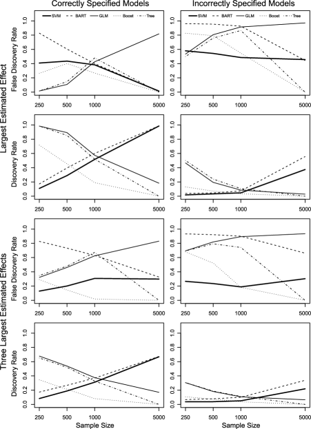
Figure 1: False discovery rate (FDR) and discovery rate (DR) for selecting the best treatments among a large number of available treatments. Simulation results with correct specification (left column) and incorrect specification (right column) are shown. The figure compares the performance of the proposed method (SVM; thick solid lines) to that of BART (BART; dashed lines), conditional inference trees (Tree; dashed-dotted lines), Boosting (Boost; dotted lines), and Bayesian logistic regression with a noninformative prior (GLM; solid lines). Here, discovery is defined as estimating the largest effect (three largest effects) as the largest effect (nonzero effects) with the correct sign. The first and second (third and fourth) rows present the FDR and DR for the largest effect (three largest effects), respectively.

Figure 1 summarizes the results in terms of false discovery rate (FDR) and discovery rate (DR) separately for the largest and substantive effects. We define discovery as estimating the largest effect (three largest effects) as the largest effect (nonzero effects) with the correct sign. Similarly, false discovery occurs when the largest effect is not correctly discovered and at least one coefficient is estimated to be nonzero. FDR may not equal one minus DR because the former is based only on the simulations where at least one coefficient is estimated to be nonzero. The first row presents FDR for the largest effect whereas the second row presents its DR. Similarly, the third row plots the FDR for the three largest effects while the fourth row presents their DR. Note that fewer than three nonzero effects may be estimated.

The results show that across simulations the proposed method (SVM; solid lines) has a smaller FDR while its DR is competitive with other methods. The comparison with BART reveals a key feature of our method. The proposed method dominates BART in FDR regardless of model specification. The largest estimated effect from BART identifies the largest effect slightly more frequently, but at the cost of a higher FDR. Despite its low FDR, our method maintains a competitive DR. For many methods, model misspecification increases FDR and reduces DR. For this reason, we recommend erring in favor of including too many rather than too few pre-treatment covariates in the model.

Unlike three of its competitors, Boosting, conditional inference trees, and Bayesian GLM, the performance of the proposed method improves as the sample size increases. Boosting and trees both attain an FDR and DR of zero as the sample size grows. The tree focuses in on the largest effects, not identifying any small effects as the sample size grows. This may be due to the fact that trees do not converge asymptotically to the true conditional mean function unless the underlying function is piecewise constant (though they converge to the minimal risk) [see, e.g., Breiman et al. (1984)]. The boosting algorithm uses trees as base learners, which may be leading to the deteriorating performance in identifying small effects. The performance of Bayesian GLM also declines with increasing sample size, because we are not considering uncertainty in the posterior mean estimates. To address this issue, one must use some $p$-value based regularization, such as using a $p$-value threshold of $0.10$ (see Figure 2 in the next set of simulations for illustration).

4.2 Identifying units for which a treatment is beneficial/harmful

In the second set of simulations, we consider the problem of identifying groups of units for which a treatment is beneficial (or harmful). Here, we are interested in identifying interactions between a treatment and observed pre-treatment covariates. The key difference between this simulation and the previous one is that in the current setup causal heterogeneity variables (treatment-covariate interactions) may be correlated with each other as well as other noncausal variables. The previous simulation setting assumes that causal heterogeneity variables (treatment indicators) are independent of each other and other variables. In this simulation, we also include a comparison with the logistic regression with a single LASSO constraint and the maximal ten-fold cross-validation on the “value” statistic [Qian and Murphy (2011)]. This statistic is the expected benefit from a particular treatment rule [see also Imai and Strauss (2011)]. Note that in the previous simulation, due to a large number of treatments, cross-validation on this statistic is not feasible.

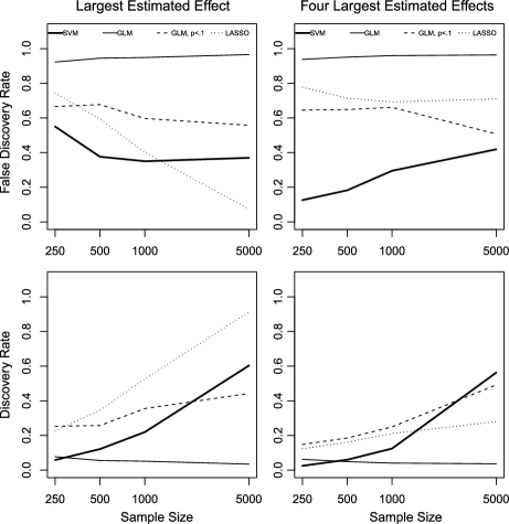
Figure 2: False discovery rate (FDR) and discovery rate (DR) for identifying units for which a treatment is most effective (or harmful). The figure compares the performance of the proposed method (SVM; solid lines) with the logistic LASSO (LASSO) and the Bayesian logistic regression based on a noninformative prior (GLM; dashed and dotted lines). For Bayesian GLM, we examine the estimates based on posterior means (dashed lines) and statistical significance ($p$-value less than $0.1$). Here, discovery is defined as estimating the largest effect (four largest effects) as the largest effect (nonzero effects) with the correct sign. The top and bottom plots in the first (second) column present the FDR and DR for the largest effect (three largest effects), respectively.

In the current simulation, we have a single treatment condition, that is, $K=1$, and 20 pre-treatment covariates $X_{i}$. The pre-treatment covariates are all based on the multivariate normal distribution with mean zero and a random variance-covariance matrix as in the previous simulation study, with five covariates then discretized using 0.5 as a threshold. Causal heterogeneity variables $Z_{i}$ consist of 20 treatment-covariate interactions plus the main effect for the treatment indicator ($L_{Z}=21$), while $V_{i}$ is composed of the main effects for the pre-treatment covariates ($L_{V}=20$).

Given this setup, we generate the outcome variable $Y_{i}$ in the same way as in Section 4.1 according to the linear probability model. There are 4 pre-treatment covariates that interact with the treatment in a systematic manner. As before, we apply an affine transformation so that an observation whose values for these two covariates are one standard deviation above the mean has the CATE of roughly $4$ and $1.7$ percentage points. That is, we set $\beta=\{-2.7,2.7,-6.7,-6.7,\ldots\}$ and $\gamma=\{50,-30,30,20,-20,\ldots\}$ where the $\ldots$ denotes uniform draws from $[-0.7,0.7]$.

Figure 2 compares the FDR and DR for our proposed method (SVM; solid lines) with those for the logistic LASSO (LASSO) and Bayesian logistic regression (GLM; dotted and dashed lines). For the Bayesian GLM, we consider two rules: one based on posterior means of coefficients (dashed lines) and the other selecting coefficients with $p$-values below $0.1$ (dotted lines). Unlike the simulations given in Section 4.1, neither BART, boosting, nor conditional inference trees provide a simple rule for variable selection in this setting and hence no results are reported.

The interpretation of these plots is identical to that of the plots in Figure 1. In the left column, the top (bottom) plot presents FDR (DR) for the largest effect, whereas that of the right column presents FDR (DR) for the four largest effects. When compared with the Bayesian GLM, the proposed method has a lower FDR for both largest and four largest estimated effects. The $p$-value thresholding improves the Bayesian GLM, and yet the proposed method maintains a much lower FDR and comparable DR. Relative to the LASSO, the proposed method is not as effective in considering the largest estimated effect except that it has a lower FDR when the sample size is small. However, when considering the four largest estimated effects, the proposed method maintains a lower FDR than the LASSO, and a comparable DR. This result is consistent with the fact that the value statistic targets the largest treatment effect while the GCV statistic corresponds to the overall fit.

To further evaluate our method, we consider a situation where each method is applied to a sample and then used to generate a treatment rule for each individual in another sample. For each method, a payoff, characterized by the net number of people in the new sample who are assigned to treatment and are in fact helped by the treatment, is calculated. To represent a budget constraint faced by most researchers, we specify the total number of individuals who can receive the treatment and vary this number within the simulation study.

Specifically, after fitting each model to an initial sample, we draw another simple random sample of 2000 observations from the same data generating process. Using the result from each method, we calculate the predicted CATE for each observation of the new sample, $\hat{\tau}(1;\widetilde{X}_{i})$, and give the treatment to those with highest predicted CATEs until the number of treated observations reaches the pre-specified limit. Finally, a payoff of the form $\mathbf{1}\{\hat{\tau}(1;\widetilde{X}_{i})>0\}\cdot\operatorname{sgn}(\tau(1;X_{i}))$ is calculated for all treated observations of the new sample where $\tau(1;X_{i})$ is the true CATE. This produces a payoff of $0.5$ if a treated observation is actually helped by the treatment, $-0.5$ if the observation is harmed, and $0$ for untreated observations. As a baseline, we compare each method to the “oracle” treatment rule, $\mathbf{1}\{\tau(1;X_{i})>0\}\cdot\operatorname{sgn}(\tau(1;X_{i}))$, which administers the treatment only when helpful. We have also considered an alternative payoff of the form $\mathbf{1}\{\hat{\tau}(1;\widetilde{X}_{i})>0\}\cdot\tau(1;X_{i})$, representing how much (rather than whether) the treatment helps or harms. The results were qualitatively similar to those presented here.

Table 4: Performance in payoff relative to the oracle

	Sample size
Method	250	500	1000	5000
SVM	$-2$	$11$	$22$	$42$
BART	$-19$	$-4$	$8$	$21$
LASSO	$-18$	$2$	$15$	$28$
GLM	$-20$	$-7$	$7$	$34$
Boost	$-1$	$10$	$18$	$40$
Tree	$2$	$2$	$2$	$5$
Treat everyone	$-123$	$-121$	$-121$	$-116$

[]Note: The table presents a payoff for each method as a percentage of the optimal oracle rule, which is considered as $100\%$. Each method is fit to a training set, and the treatment is administered to every person in the validation set with a predicted improvement. The proposed method (SVM) narrowly dominates Boosting (Boost), and both the proposed method and Boosting noticeably outperform all other competitors, except conditional inference trees (Tree) at sample size 250. At larger sample sizes the tree severely underfits. While the proposed method and Boosting perform similarly by a predictive criterion, Boosting does not return an interpretable model. BART, GLM, and LASSO represent the Bayesian Additive Regression Tree, the logistic regression with a noninformative prior, and the logistic regression with a single LASSO constraint and cross-validation on the value statistic. The bottom row presents the outcome if every observation were treated, indicating that in this simulation the average treatment effect is negative, but there exists a subgroup for which the treatment is beneficial.

The results from the simulation are presented in Table 4. The table presents a comparison of payoffs, by method, as a percentage of the optimal oracle rule, which is considered as $100\%$. The bottom row presents the outcome if every observation were treated, indicating that in this simulation the average treatment effect is negative but there exists a subgroup for which treatment is beneficial. The proposed method (SVM) narrowly dominates Boosting (Boost), and both the proposed method and Boosting noticeably outperform all other competitors, except conditional inference trees (Tree) at sample size 250. At larger sample sizes, however, the tree severely underfits. While the proposed method and Boosting perform similarly by a predictive criterion, Boosting does not return an interpretable model. We also find that SVM outperforms LASSO, which is consistent with the fact that the GCV statistic targets the overall performance while the value statistic focuses on the largest treatment effect. If administering the treatment is costless, the proposed method generates the most beneficial treatment rule among its competitors.

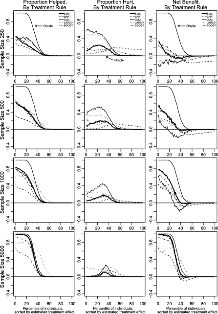
Figure 3: The relative performance of individualized treatment rules derived by each method. The figure presents the proportion of treated units (based on the treatment rule of each method) who benefit from the treatment (left column), are harmed by the treatment (middle column), and the difference between the two (right column) at each percentile of the total sample who can be assigned to the treatment. The oracle (solid lines) treats each observation only when helpful and hence is identical to the horizontal line at zero in the middle column. The proposed method (SVM; solid thick lines) makes fewer mistreatments than other methods, while it is conservative in assigning observations to the treatment.

Figure 3 presents the results across methods and sample sizes in the presence of a budget constraint. The left column shows the proportion of treated units that actually benefit from the treatment for each observation considered for the treatment in the order of predicted CATE (the horizontal axis). The oracle identifies those who certainly benefit from the treatment and treats them first. The middle column shows the proportion of treated units that are hurt by the treatment. Here, the oracle never hurts observations and hence is represented by the horizontal line at zero. The right column presents the net benefit by treatment rule, which can be calculated as the difference between the positive (left column) and negative (middle column) effects. Each row presents a different sample size to which each method is applied.

The figure shows that when the sample size is small, the proposed method assigns fewer observations a harmful treatment, relative to its competitors. For moderate and large sample sizes, the proposed method dominates its competitors in both identifying a group that would benefit from the treatment and avoiding treating those who would be hurt. This can be seen from the plots in the middle column where the result based on the proposed method (SVM; solid thick lines) stays close to the horizontal zero line when compared to other methods. Similarly, in the right column, the results based on the proposed method stay above other methods. When these lines go below zero, it implies that a majority of treated observations would be harmed by the treatment. The disadvantage of the proposed method is its conservativeness. This can be seen in the left column where at the beginning of the percentile the solid thick line is below its competitors for small sample sizes. This difference vanishes as the sample size increases, with the proposed method outperforming its competitors. In sum, when used to predict a treatment rule for out-of-sample observations, the proposed method makes fewer harmful prescriptions and often yields a larger net benefit than its competitors.

5 Concluding remarks

Estimation of heterogeneous treatment effects plays an essential role in scientific research and policy making. In particular, researchers often wish to select the most efficacious treatments from a large number of possible treatments and to identify individuals who benefit most (or are harmed) by treatments. Estimation of treatment effect heterogeneity is also important when generalizing experimental results to a target population of interest.

The key insight of this paper is to formulate the identification of heterogeneous treatment effects as a variable selection problem. Within this framework, we develop a Support Vector Machine with two separate sparsity constraints, one for a set of treatment effect heterogeneity parameters of interest and the other for observed pre-treatment effect parameters. This setup addresses the fact that in many applications, pre-treatment covariates are much more powerful predictors than treatment variables of interest or their interactions with covariates. In addition, unlike the existing techniques such as Boosting and BART, the proposed method yields a parsimonious model that is easy to interpret. Our simulation studies show that the proposed method has low false discovery rates while maintaining competitive discovery rates. The simulation study also shows that the use of our GCV statistic is appropriate when exploring the treatment effect heterogeneity rather than identifying the single optimal treatment rule.

Table 5: Nonzero coefficient estimates for the New Haven get-out-the-vote experiment

Treatment interactions
Visit	Phone	Mailings	Message	Coefficient
Yes	Any	0–3	Any	$1.50$
No	No	2	Neighborhood	$1.25$
Yes	No	0	Any	$1.04$
No	Close	0	Close	$0.84$
Any	No	3	Any	$0.72$
Yes	Any	0	Any	$0.59$
Any	No	3	Civic	$0.49$
Yes	No	0–3	Close	$0.15$
No	Any	2	Any	$-0.08$
Any	Any	3	Civic	$-0.68$
Any	Civic	0–3	Civic	$-0.95$
No	No	2	Close	$-2.09$
Any	Civic/Blood	0–3	Civic	$-2.16$
No	Neighbor	0–3	Neighbor	$-2.72$
No	Civic	0–3	Neighbor	$-3.67$

[]Note: Coefficients are presented on the percentage point scale. 13 of the 193 causal heterogeneity parameters were estimated as nonzero ($6.7\%$). The largest positive coefficients correspond with a personal visit, while the largest negative effects correspond with receiving a civic or neighborhood solidarity appeal via phone. These coefficients generate the predicted treatment effects in Table 1.

Table 6: Nonzero coefficient estimates for the job training program data

	NSW	PSID
Treatment intercept	$6.92$	$6.67$
Main effects
Age	$0.00$	$-0.83$
Married	$1.32$	$3.39$
White	$0.00$	$0.10$
Squared terms
Age2	$-0.03$	$-0.09$
Education2	$0.89$	$0.86$
Interaction terms
No HS degree, Unemployed in 1975	$-1.06$	$0.00$
White, Married	$0.00$	$26.16$
White, No HS degree	$25.35$	$30.65$
Hispanic, Logged 1975 earnings	$-49.36$	$-62.15$
Black, Logged 1975 earnings	$8.29$	$0.00$
White, Education	$0.00$	$-1.41$
Married, Education	$4.90$	$12.11$
Married, Logged 1975 earnings	$0.00$	$5.72$
Education, Unemployed in 1975	$7.52$	$9.59$
Age, Education	$0.00$	$-0.47$
Age, Black	$-0.56$	$0.00$
Age, Hispanic	$0.00$	$0.34$
Age, Unemployed in 1975	$3.30$	$4.79$

[]Note: The table presents the estimates from the model fitted to the NSW Data without (left column) and with the PSID weights (right column). Coefficients are rescaled to the percentage point scale. The first row contains the estimated intercept, which corresponds to the estimated CATE for an observation with characteristics set at the mean of all pre-treatment covariates.

A number of extensions of the method developed in this paper are possible. For example, we can accommodate other types of outcome variables by considering different loss functions. Instead of the GCV statistic we use, alternative criteria such as AIC or BIC statistics as well as more targeted quantities such as the average treatment effect for the target population can be employed. While we use LASSO constraints, researchers may prefer alternative penalty functions such as the SCAD or adaptive LASSO penalty. Furthermore, although not directly examined in this paper, the proposed method can be extended to the situation where the goal is to choose the best treatment for each individual from multiple alternative treatments. Finally, it is of interest to consider how the proposed method can be applied to observational data [e.g., see Zhang et al. (2012) who develop a doubly robust estimator for optimal treatment regimes] and longitudinal data settings where the derivation of optimal dynamic treatment regimes is a frequent goal [e.g., Murphy (2003), Zhao et al. (2011)]. The development of such methods helps applied researchers avoid the use of ad hoc subgroup analysis and identify treatment effect heterogeneity in a statistically principled manner.

Appendix: Estimated nonzero coefficients for empirical applications

Acknolwedgments

An earlier version of this paper was circulated under the title of “Identifying Treatment Effect Heterogeneity through Optimal Classification and Variable Selection” and received the Tom Ten Have Memorial Award at the 2011 Atlantic Causal Inference Conference. We thank Charles Elkan, Jake Bowers, Kentaro Fukumoto, Holger Kern, Michael Rosenbaum, and Sherry Zaks for useful comments. The Editor, Associate Editor, and two anonymous reviewers provided useful advice.

References

- Bradley and Mangasarian (1998) {bincollection}[auto:STB—2012/11/05—08:49:14] \bauthor\bsnmBradley, \bfnmP.\binitsP. and \bauthor\bsnmMangasarian, \bfnmO. L.\binitsO. L. (\byear1998). \btitleFeature selection via concave minimization and support vector machines. In \bbooktitleMachine Learning Proceedings of the Fifteenth International Conference \bpages82–90. \bpublisherMorgan Kaufmann, \blocationSan Francisco, CA. \bptokimsref \endbibitem
- Breiman et al. (1984) {bbook}[mr] \bauthor\bsnmBreiman, \bfnmLeo\binitsL., \bauthor\bsnmFriedman, \bfnmJerome H.\binitsJ. H., \bauthor\bsnmOlshen, \bfnmRichard A.\binitsR. A. and \bauthor\bsnmStone, \bfnmCharles J.\binitsC. J. (\byear1984). \btitleClassification and Regression Trees. \bpublisherWadsworth Advanced Books and Software, \blocationBelmont, CA. \bidmr=0726392 \bptokimsref \endbibitem
- Cai et al. (2011) {barticle}[pbm] \bauthor\bsnmCai, \bfnmTianxi\binitsT., \bauthor\bsnmTian, \bfnmLu\binitsL., \bauthor\bsnmWong, \bfnmPeggy H.\binitsP. H. and \bauthor\bsnmWei, \bfnmL. J.\binitsL. J. (\byear2011). \btitleAnalysis of randomized comparative clinical trial data for personalized treatment selections. \bjournalBiostatistics \bvolume12 \bpages270–282. \biddoi=10.1093/biostatistics/kxq060, issn=1468-4357, pii=kxq060, pmcid=3062150, pmid=20876663 \bptokimsref \endbibitem
- Chipman, George and McCulloch (2010) {barticle}[mr] \bauthor\bsnmChipman, \bfnmHugh A.\binitsH. A., \bauthor\bsnmGeorge, \bfnmEdward I.\binitsE. I. and \bauthor\bsnmMcCulloch, \bfnmRobert E.\binitsR. E. (\byear2010). \btitleBart: Bayesian additive regression trees. \bjournalAnn. Appl. Stat. \bvolume4 \bpages266–298. \biddoi=10.1214/09-AOAS285, issn=1932-6157, mr=2758172 \bptokimsref \endbibitem
- Cole and Stuart (2010) {barticle}[pbm] \bauthor\bsnmCole, \bfnmStephen R.\binitsS. R. and \bauthor\bsnmStuart, \bfnmElizabeth A.\binitsE. A. (\byear2010). \btitleGeneralizing evidence from randomized clinical trials to target populations: The ACTG 320 trial. \bjournalAm. J. Epidemiol. \bvolume172 \bpages107–115. \biddoi=10.1093/aje/kwq084, issn=1476-6256, pii=kwq084, pmcid=2915476, pmid=20547574 \bptokimsref \endbibitem
- Crump et al. (2008) {barticle}[auto:STB—2012/11/05—08:49:14] \bauthor\bsnmCrump, \bfnmR. K.\binitsR. K., \bauthor\bsnmHotz, \bfnmV. J.\binitsV. J., \bauthor\bsnmImbens, \bfnmG. W.\binitsG. W. and \bauthor\bsnmMitnik, \bfnmO. A.\binitsO. A. (\byear2008). \btitleNonparametric tests for treatment effect heterogeneity. \bjournalThe Review of Economics and Statistics \bvolume90 \bpages389–405. \bptokimsref \endbibitem
- Davison (1992) {barticle}[auto:STB—2012/11/05—08:49:14] \bauthor\bsnmDavison, \bfnmA. C.\binitsA. C. (\byear1992). \btitleTreatment effect heterogeneity in paired data. \bjournalBiometrika \bvolume79 \bpages463–474. \bptokimsref \endbibitem
- Dehejia and Wahba (1999) {barticle}[auto:STB—2012/11/05—08:49:14] \bauthor\bsnmDehejia, \bfnmR. H.\binitsR. H. and \bauthor\bsnmWahba, \bfnmS.\binitsS. (\byear1999). \btitleCausal effects in nonexperimental studies: Reevaluating the evaluation of training programs. \bjournalJ. Amer. Statist. Assoc. \bvolume94 \bpages1053–1062. \bptokimsref \endbibitem
- Efron et al. (2004) {barticle}[mr] \bauthor\bsnmEfron, \bfnmBradley\binitsB., \bauthor\bsnmHastie, \bfnmTrevor\binitsT., \bauthor\bsnmJohnstone, \bfnmIain\binitsI. and \bauthor\bsnmTibshirani, \bfnmRobert\binitsR. (\byear2004). \btitleLeast angle regression. \bjournalAnn. Statist. \bvolume32 \bpages407–499. \biddoi=10.1214/009053604000000067, issn=0090-5364, mr=2060166 \bptnotecheck related\bptokimsref \endbibitem
- Franc, Zien and Schölkopf (2011) {bmisc}[auto:STB—2012/11/05—08:49:14] \bauthor\bsnmFranc, \bfnmV.\binitsV., \bauthor\bsnmZien, \bfnmA.\binitsA. and \bauthor\bsnmSchölkopf, \bfnmB.\binitsB. (\byear2011). \bhowpublishedSupport vector machines as probabilistic models. In The 28th International Conference on Machine Learning 665–672. ACM, Bellevue, WA. \bptokimsref \endbibitem
- Frangakis (2009) {barticle}[pbm] \bauthor\bsnmFrangakis, \bfnmConstantine\binitsC. (\byear2009). \btitleThe calibration of treatment effects from clinical trials to target populations. \bjournalClin. Trials \bvolume6 \bpages136–140. \biddoi=10.1177/1740774509103868, issn=1740-7745, pii=6/2/136, pmid=19342466 \bptokimsref \endbibitem
- Freund and Schapire (1999) {bincollection}[auto:STB—2012/11/05—08:49:14] \bauthor\bsnmFreund, \bfnmY.\binitsY. and \bauthor\bsnmSchapire, \bfnmR. E.\binitsR. E. (\byear1999). \btitleA short introduction to boosting. In \bbooktitleProceedings of the Sixteenth International Joint Conference on Artificial Intelligence \bpages1401–1406. \bpublisherMorgan Kaufmann, \blocationSan Francisco, CA. \bptokimsref \endbibitem
- Friedman, Hastie and Tibshirani (2010) {barticle}[auto:STB—2012/11/05—08:49:14] \bauthor\bsnmFriedman, \bfnmJ. H.\binitsJ. H., \bauthor\bsnmHastie, \bfnmT.\binitsT. and \bauthor\bsnmTibshirani, \bfnmR.\binitsR. (\byear2010). \btitleRegularization paths for generalized linear models via coordinate descent. \bjournalJournal of Statistical Software \bvolume33 \bpages1–22. \bptokimsref \endbibitem
- Gail and Simon (1985) {barticle}[pbm] \bauthor\bsnmGail, \bfnmM.\binitsM. and \bauthor\bsnmSimon, \bfnmR.\binitsR. (\byear1985). \btitleTesting for qualitative interactions between treatment effects and patient subsets. \bjournalBiometrics \bvolume41 \bpages361–372. \bidissn=0006-341X, pmid=4027319 \bptokimsref \endbibitem
- Gelman et al. (2008) {barticle}[mr] \bauthor\bsnmGelman, \bfnmAndrew\binitsA., \bauthor\bsnmJakulin, \bfnmAleks\binitsA., \bauthor\bsnmPittau, \bfnmMaria Grazia\binitsM. G. and \bauthor\bsnmSu, \bfnmYu-Sung\binitsY.-S. (\byear2008). \btitleA weakly informative default prior distribution for logistic and other regression models. \bjournalAnn. Appl. Stat. \bvolume2 \bpages1360–1383. \biddoi=10.1214/08-AOAS191, issn=1932-6157, mr=2655663 \bptokimsref \endbibitem
- Gerber and Green (2000) {barticle}[auto:STB—2012/11/05—08:49:14] \bauthor\bsnmGerber, \bfnmA. S.\binitsA. S. and \bauthor\bsnmGreen, \bfnmD. P.\binitsD. P. (\byear2000). \btitleThe effects of canvassing, telephone calls, and direct mail on voter turnout: A field experiment. \bjournalAmerican Political Science Review \bvolume94 \bpages653–663. \bptokimsref \endbibitem
- Gerber, Green and Larimer (2008) {barticle}[auto:STB—2012/11/05—08:49:14] \bauthor\bsnmGerber, \bfnmA.\binitsA., \bauthor\bsnmGreen, \bfnmD.\binitsD. and \bauthor\bsnmLarimer, \bfnmC.\binitsC. (\byear2008). \btitleSocial pressure and voter turnout: Evidence from a large-scale field experiment. \bjournalAmerican Political Science Review \bvolume102 \bpages33–48. \bptokimsref \endbibitem
- Green and Kern (2010a) {bmisc}[auto:STB—2012/11/05—08:49:14] \bauthor\bsnmGreen, \bfnmD. P.\binitsD. P. and \bauthor\bsnmKern, \bfnmH. L.\binitsH. L. (\byear2010a). \bhowpublishedDetecting heterogenous treatment effects in large-scale experiments using Bayesian additive regression trees. In The Annual Summer Meeting of the Society of Political Methodology. Univ. Iowa. \bptokimsref \endbibitem
- Green and Kern (2010b) {bmisc}[auto:STB—2012/11/05—08:49:14] \bauthor\bsnmGreen, \bfnmD. P.\binitsD. P. and \bauthor\bsnmKern, \bfnmH. L.\binitsH. L. (\byear2010b). \bhowpublishedGeneralizing experimental results. In The Annual Meeting of the American Political Science Association. Washington, D.C. \bptokimsref \endbibitem
- Gunter, Zhu and Murphy (2011) {barticle}[mr] \bauthor\bsnmGunter, \bfnmL.\binitsL., \bauthor\bsnmZhu, \bfnmJ.\binitsJ. and \bauthor\bsnmMurphy, \bfnmS. A.\binitsS. A. (\byear2011). \btitleVariable selection for qualitative interactions. \bjournalStat. Methodol. \bvolume8 \bpages42–55. \biddoi=10.1016/j.stamet.2009.05.003, issn=1572-3127, mr=2741508 \bptokimsref \endbibitem
- Hartman, Grieve and Sekhon (2010) {bmisc}[auto:STB—2012/11/05—08:49:14] \bauthor\bsnmHartman, \bfnmE.\binitsE., \bauthor\bsnmGrieve, \bfnmR.\binitsR. and \bauthor\bsnmSekhon, \bfnmJ. S.\binitsJ. S. (\byear2010). \bhowpublishedFrom SATE to PATT: The essential role of placebo test combining experimental and observational studies. In The Annual Meeting of the American Political Science Association. Washington, D.C. \bptokimsref \endbibitem
- Hill (2011) {barticle}[auto:STB—2012/11/05—08:49:14] \bauthor\bsnmHill, \bfnmJ. L.\binitsJ. L. (\byear2011). \btitleChallenges with propensity score matching in a high-dimensional setting and a potential alternative. \bjournalMultivariate and Behavioral Research \bvolume46 \bpages477–513. \bptokimsref \endbibitem
- Hothorn, Hornik and Zeileis (2006) {barticle}[mr] \bauthor\bsnmHothorn, \bfnmTorsten\binitsT., \bauthor\bsnmHornik, \bfnmKurt\binitsK. and \bauthor\bsnmZeileis, \bfnmAchim\binitsA. (\byear2006). \btitleUnbiased recursive partitioning: A conditional inference framework. \bjournalJ. Comput. Graph. Statist. \bvolume15 \bpages651–674. \biddoi=10.1198/106186006X133933, issn=1061-8600, mr=2291267 \bptokimsref \endbibitem
- Imai (2005) {barticle}[auto:STB—2012/11/05—08:49:14] \bauthor\bsnmImai, \bfnmK.\binitsK. (\byear2005). \btitleDo get-out-the-vote calls reduce turnout?: The importance of statistical methods for field experiments. \bjournalAmerican Political Science Review \bvolume99 \bpages283–300. \bptokimsref \endbibitem
- Imai and Strauss (2011) {barticle}[auto:STB—2012/11/05—08:49:14] \bauthor\bsnmImai, \bfnmK.\binitsK. and \bauthor\bsnmStrauss, \bfnmA.\binitsA. (\byear2011). \btitleEstimation of heterogeneous treatment effects from randomized experiments, with application to the optimal planning of the get-out-the-vote campaign. \bjournalPolitical Analysis \bvolume19 \bpages1–19. \bptokimsref \endbibitem
- Kang et al. (2012) {barticle}[mr] \bauthor\bsnmKang, \bfnmJoseph\binitsJ., \bauthor\bsnmSu, \bfnmXiaogang\binitsX., \bauthor\bsnmHitsman, \bfnmBrian\binitsB., \bauthor\bsnmLiu, \bfnmKiang\binitsK. and \bauthor\bsnmLloyd-Jones, \bfnmDonald\binitsD. (\byear2012). \btitleTree-structured analysis of treatment effects with large observational data. \bjournalJ. Appl. Stat. \bvolume39 \bpages513–529. \biddoi=10.1080/02664763.2011.602056, issn=0266-4763, mr=2880431 \bptokimsref \endbibitem
- Lagakos (2006) {barticle}[pbm] \bauthor\bsnmLagakos, \bfnmStephen W.\binitsS. W. (\byear2006). \btitleThe challenge of subgroup analyses–reporting without distorting. \bjournalN. Engl. J. Med. \bvolume354 \bpages1667–1669. \biddoi=10.1056/NEJMp068070, issn=1533-4406, pii=354/16/1667, pmid=16625007 \bptokimsref \endbibitem
- LaLonde (1986) {barticle}[auto:STB—2012/11/05—08:49:14] \bauthor\bsnmLaLonde, \bfnmR. J.\binitsR. J. (\byear1986). \btitleEvaluating the econometric evaluations of training programs with experimental data. \bjournalAmerican Economic Review \bvolume76 \bpages604–620. \bptokimsref \endbibitem
- LeBlanc and Kooperberg (2010) {barticle}[auto:STB—2012/11/05—08:49:14] \bauthor\bsnmLeBlanc, \bfnmM.\binitsM. and \bauthor\bsnmKooperberg, \bfnmC.\binitsC. (\byear2010). \btitleBoosting predictions of treatment success. \bjournalProc. Natl. Acad. Sci. USA \bvolume107 \bpages13559–13560. \bptokimsref \endbibitem
- Lee, Lin and Wahba (2004) {barticle}[mr] \bauthor\bsnmLee, \bfnmYoonkyung\binitsY., \bauthor\bsnmLin, \bfnmYi\binitsY. and \bauthor\bsnmWahba, \bfnmGrace\binitsG. (\byear2004). \btitleMulticategory support vector machines: Theory and application to the classification of microarray data and satellite radiance data. \bjournalJ. Amer. Statist. Assoc. \bvolume99 \bpages67–81. \biddoi=10.1198/016214504000000098, issn=0162-1459, mr=2054287 \bptokimsref \endbibitem
- Lin (2002) {barticle}[mr] \bauthor\bsnmLin, \bfnmYi\binitsY. (\byear2002). \btitleSupport vector machines and the Bayes rule in classification. \bjournalData Min. Knowl. Discov. \bvolume6 \bpages259–275. \biddoi=10.1023/A:1015469627679, issn=1384-5810, mr=1917926 \bptokimsref \endbibitem
- Lipkovich et al. (2011) {barticle}[mr] \bauthor\bsnmLipkovich, \bfnmIlya\binitsI., \bauthor\bsnmDmitrienko, \bfnmAlex\binitsA., \bauthor\bsnmDenne, \bfnmJonathan\binitsJ. and \bauthor\bsnmEnas, \bfnmGregory\binitsG. (\byear2011). \btitleSubgroup identification based on differential effect search—a recursive partitioning method for establishing response to treatment in patient subpopulations. \bjournalStat. Med. \bvolume30 \bpages2601–2621. \biddoi=10.1002/sim.4289, issn=0277-6715, mr=2815438 \bptokimsref \endbibitem
- Loh et al. (2012) {barticle}[auto:STB—2012/11/05—08:49:14] \bauthor\bsnmLoh, \bfnmW. Y.\binitsW. Y., \bauthor\bsnmPiper, \bfnmM. E.\binitsM. E., \bauthor\bsnmSchlam, \bfnmT. R.\binitsT. R., \bauthor\bsnmFiore, \bfnmM. C.\binitsM. C., \bauthor\bsnmSmith, \bfnmS. S.\binitsS. S., \bauthor\bsnmJorenby, \bfnmD. E.\binitsD. E., \bauthor\bsnmCook, \bfnmJ. W.\binitsJ. W., \bauthor\bsnmBolt, \bfnmD. M.\binitsD. M. and \bauthor\bsnmBaker, \bfnmT. B.\binitsT. B. (\byear2012). \btitleShould all smokers use combination smoking cessation pharmacotherapy? Using novel analytic methods to detect differential treatment effects over eight weeks of pharmacotherapy. \bjournalNicotine and Tobacco Research \bvolume14 \bpages131–141. \bptokimsref \endbibitem
- Manski (2004) {barticle}[mr] \bauthor\bsnmManski, \bfnmCharles F.\binitsC. F. (\byear2004). \btitleStatistical treatment rules for heterogeneous populations. \bjournalEconometrica \bvolume72 \bpages1221–1246. \biddoi=10.1111/j.1468-0262.2004.00530.x, issn=0012-9682, mr=2064712 \bptokimsref \endbibitem
- Menon et al. (2012) {bmisc}[auto:STB—2012/11/05—08:49:14] \bauthor\bsnmMenon, \bfnmA. K.\binitsA. K., \bauthor\bsnmJiang, \bfnmX.\binitsX., \bauthor\bsnmVembu, \bfnmS.\binitsS., \bauthor\bsnmElkan, \bfnmC.\binitsC. and \bauthor\bsnmOhno-Machado, \bfnmL.\binitsL. (\byear2012). \bhowpublishedPredicting accurate probabilities with a ranking loss. In Proceedings of the 29th International Conference on Machine Learning. Edinburgh, Scotland. \bptokimsref \endbibitem
- Moodie, Platt and Kramer (2009) {barticle}[mr] \bauthor\bsnmMoodie, \bfnmErica E. M.\binitsE. E. M., \bauthor\bsnmPlatt, \bfnmRobert W.\binitsR. W. and \bauthor\bsnmKramer, \bfnmMichael S.\binitsM. S. (\byear2009). \btitleEstimating response-maximized decision rules with applications to breastfeeding. \bjournalJ. Amer. Statist. Assoc. \bvolume104 \bpages155–165. \biddoi=10.1198/jasa.2009.0011, issn=0162-1459, mr=2663039 \bptokimsref \endbibitem
- Murphy (2003) {barticle}[mr] \bauthor\bsnmMurphy, \bfnmS. A.\binitsS. A. (\byear2003). \btitleOptimal dynamic treatment regimes. \bjournalJ. R. Stat. Soc. Ser. B Stat. Methodol. \bvolume65 \bpages331–366. \biddoi=10.1111/1467-9868.00389, issn=1369-7412, mr=1983752 \bptnotecheck related\bptokimsref \endbibitem
- Nickerson (2008) {barticle}[auto:STB—2012/11/05—08:49:14] \bauthor\bsnmNickerson, \bfnmD. W.\binitsD. W. (\byear2008). \btitleIs voting contagious?: Evidence from two field experiments. \bjournalAmerican Political Science Review \bvolume102 \bpages49–57. \bptokimsref \endbibitem
- Pineau et al. (2007) {barticle}[auto:STB—2012/11/05—08:49:14] \bauthor\bsnmPineau, \bfnmJ.\binitsJ., \bauthor\bsnmBellemare, \bfnmM. G.\binitsM. G., \bauthor\bsnmRush, \bfnmA. J.\binitsA. J., \bauthor\bsnmGhizaru, \bfnmA.\binitsA. and \bauthor\bsnmMurphy, \bfnmS. A.\binitsS. A. (\byear2007). \btitleConstructing evidence-based treatment strategies using methods from computer science. \bjournalDrug and Alcohol Dependence \bvolume88S \bpagesS52–S60. \bptokimsref \endbibitem
- Platt (1999) {bmisc}[auto:STB—2012/11/05—08:49:14] \bauthor\bsnmPlatt, \bfnmJ.\binitsJ. (\byear1999). \bhowpublishedProbabilistic outputs for support vector machines and comparison to regularized likelihood methods. In Advances in Large Margin Classifiers 61–74. MIT Press, Cambridge, MA. \bptokimsref \endbibitem
- Qian and Murphy (2011) {barticle}[mr] \bauthor\bsnmQian, \bfnmMin\binitsM. and \bauthor\bsnmMurphy, \bfnmSusan A.\binitsS. A. (\byear2011). \btitlePerformance guarantees for individualized treatment rules. \bjournalAnn. Statist. \bvolume39 \bpages1180–1210. \biddoi=10.1214/10-AOS864, issn=0090-5364, mr=2816351 \bptokimsref \endbibitem
- Ratkovic and Imai (2012) {bmisc}[auto] \bauthor\bsnmRatkovic, \bfnmM.\binitsM. and \bauthor\bsnmImai, \bfnmK.\binitsK. (\byear2012). \bhowpublishedFindIt: R package for finding heterogeneous treatment effects. Available at Comprehensive R Archive Network (http://cran.r-project.org/ package=FindIt). \bptokimsref \endbibitem
- Rosenbaum and Rubin (1983) {barticle}[mr] \bauthor\bsnmRosenbaum, \bfnmPaul R.\binitsP. R. and \bauthor\bsnmRubin, \bfnmDonald B.\binitsD. B. (\byear1983). \btitleThe central role of the propensity score in observational studies for causal effects. \bjournalBiometrika \bvolume70 \bpages41–55. \biddoi=10.1093/biomet/70.1.41, issn=0006-3444, mr=0742974 \bptokimsref \endbibitem
- Rothwell (2005) {barticle}[auto:STB—2012/11/05—08:49:14] \bauthor\bsnmRothwell, \bfnmP. M.\binitsP. M. (\byear2005). \btitleSubgroup analysis in randomized controlled trials: Importance, indications, and interpretation. \bjournalThe Lancet \bvolume365 \bpages176–186. \bptokimsref \endbibitem
- Rubin (1990) {barticle}[mr] \bauthor\bsnmRubin, \bfnmDonald B.\binitsD. B. (\byear1990). \btitleComment on J. Neyman and causal inference in experiments and observational studies: “On the application of probability theory to agricultural experiments. Essay on principles. Section 9” [Ann. Agric. Sci. 10 (1923) 1–51]. \bjournalStatist. Sci. \bvolume5 \bpages472–480. \bidissn=0883-4237, mr=1092987 \bptnotecheck related\bptokimsref \endbibitem
- Sollich (2002) {barticle}[auto:STB—2012/11/05—08:49:14] \bauthor\bsnmSollich, \bfnmP.\binitsP. (\byear2002). \btitleBayesian methods for support vector machines: Evidence and predictive class probabilities. \bjournalMachine Learning \bvolume46 \bpages21–52. \bptokimsref \endbibitem
- Stuart et al. (2011) {barticle}[mr] \bauthor\bsnmStuart, \bfnmElizabeth A.\binitsE. A., \bauthor\bsnmCole, \bfnmStephen R.\binitsS. R., \bauthor\bsnmBradshaw, \bfnmCatherine P.\binitsC. P. and \bauthor\bsnmLeaf, \bfnmPhilip J.\binitsP. J. (\byear2011). \btitleThe use of propensity scores to assess the generalizability of results from randomized trials. \bjournalJ. Roy. Statist. Soc. Ser. A \bvolume174 \bpages369–386. \biddoi=10.1111/j.1467-985X.2010.00673.x, issn=0964-1998, mr=2898850 \bptokimsref \endbibitem
- Su et al. (2009) {barticle}[auto:STB—2012/11/05—08:49:14] \bauthor\bsnmSu, \bfnmX.\binitsX., \bauthor\bsnmTsai, \bfnmC. L.\binitsC. L., \bauthor\bsnmWang, \bfnmH.\binitsH., \bauthor\bsnmNickerson, \bfnmD. M.\binitsD. M. and \bauthor\bsnmLi, \bfnmB.\binitsB. (\byear2009). \btitleSubgroup analysis via recursive partitioning. \bjournalJ. Mach. Learn. Res. \bvolume10 \bpages141–158. \bptokimsref \endbibitem
- Tibshirani (1996) {barticle}[mr] \bauthor\bsnmTibshirani, \bfnmRobert\binitsR. (\byear1996). \btitleRegression shrinkage and selection via the lasso. \bjournalJ. Roy. Statist. Soc. Ser. B \bvolume58 \bpages267–288. \bidissn=0035-9246, mr=1379242 \bptokimsref \endbibitem
- Vapnik (1995) {bbook}[mr] \bauthor\bsnmVapnik, \bfnmVladimir N.\binitsV. N. (\byear1995). \btitleThe Nature of Statistical Learning Theory. \bpublisherSpringer, \blocationNew York. \bidmr=1367965 \bptokimsref \endbibitem
- Wahba (1990) {bbook}[mr] \bauthor\bsnmWahba, \bfnmGrace\binitsG. (\byear1990). \btitleSpline Models for Observational Data. \bseriesCBMS-NSF Regional Conference Series in Applied Mathematics \bvolume59. \bpublisherSIAM, \blocationPhiladelphia, PA. \biddoi=10.1137/1.9781611970128, mr=1045442 \bptokimsref \endbibitem
- Wahba (2002) {barticle}[mr] \bauthor\bsnmWahba, \bfnmGrace\binitsG. (\byear2002). \btitleSoft and hard classification by reproducing kernel Hilbert space methods. \bjournalProc. Natl. Acad. Sci. USA \bvolume99 \bpages16524–16530 (electronic). \biddoi=10.1073/pnas.242574899, issn=1091-6490, mr=1947755 \bptokimsref \endbibitem
- Yang and Zou (2012) {bmisc}[auto:STB—2012/11/05—08:49:14] \bauthor\bsnmYang, \bfnmY.\binitsY. and \bauthor\bsnmZou, \bfnmH.\binitsH. (\byear2012). \bhowpublishedAn efficient algorithm for computing the HHSVM and its generalizations. J. Comput. Graph. Statist. To appear. \bptokimsref \endbibitem
- Yuan and Lin (2006) {barticle}[mr] \bauthor\bsnmYuan, \bfnmMing\binitsM. and \bauthor\bsnmLin, \bfnmYi\binitsY. (\byear2006). \btitleModel selection and estimation in regression with grouped variables. \bjournalJ. R. Stat. Soc. Ser. B Stat. Methodol. \bvolume68 \bpages49–67. \biddoi=10.1111/j.1467-9868.2005.00532.x, issn=1369-7412, mr=2212574 \bptokimsref \endbibitem
- Zhang (2004) {barticle}[mr] \bauthor\bsnmZhang, \bfnmTong\binitsT. (\byear2004). \btitleStatistical behavior and consistency of classification methods based on convex risk minimization. \bjournalAnn. Statist. \bvolume32 \bpages56–85. \biddoi=10.1214/aos/1079120130, issn=0090-5364, mr=2051001 \bptokimsref \endbibitem
- Zhang (2006) {barticle}[mr] \bauthor\bsnmZhang, \bfnmHao Helen\binitsH. H. (\byear2006). \btitleVariable selection for support vector machines via smoothing spline ANOVA. \bjournalStatist. Sinica \bvolume16 \bpages659–674. \bidissn=1017-0405, mr=2267254 \bptokimsref \endbibitem
- Zhang et al. (2012) {bmisc}[auto:STB—2012/11/05—08:49:14] \bauthor\bsnmZhang, \bfnmB.\binitsB., \bauthor\bsnmTsiatis, \bfnmA. A.\binitsA. A., \bauthor\bsnmLaber, \bfnmE. B.\binitsE. B. and \bauthor\bsnmDavidian, \bfnmM.\binitsM. (\byear2012). \bhowpublishedA robust method for estimating optimal treatment regimes. Biometrics. To appear. \bptokimsref \endbibitem
- Zhao et al. (2011) {barticle}[mr] \bauthor\bsnmZhao, \bfnmYufan\binitsY., \bauthor\bsnmZeng, \bfnmDonglin\binitsD., \bauthor\bsnmSocinski, \bfnmMark A.\binitsM. A. and \bauthor\bsnmKosorok, \bfnmMichael R.\binitsM. R. (\byear2011). \btitleReinforcement learning strategies for clinical trials in nonsmall cell lung cancer. \bjournalBiometrics \bvolume67 \bpages1422–1433. \biddoi=10.1111/j.1541-0420.2011.01572.x, issn=0006-341X, mr=2872393 \bptokimsref \endbibitem
- Zhao et al. (2012) {barticle}[auto:STB—2012/11/05—08:49:14] \bauthor\bsnmZhao, \bfnmY.\binitsY., \bauthor\bsnmZeng, \bfnmD.\binitsD., \bauthor\bsnmRush, \bfnmJ. A.\binitsJ. A. and \bauthor\bsnmKosorok, \bfnmM. R.\binitsM. R. (\byear2012). \btitleEstimating individualized treatment rules using outcome weighted learning. \bjournalJ. Amer. Statist. Assoc. \bvolume107 \bpages1106–1118. \bptokimsref \endbibitem
- Zou and Hastie (2005) {barticle}[mr] \bauthor\bsnmZou, \bfnmHui\binitsH. and \bauthor\bsnmHastie, \bfnmTrevor\binitsT. (\byear2005). \btitleRegularization and variable selection via the elastic net. \bjournalJ. R. Stat. Soc. Ser. B Stat. Methodol. \bvolume67 \bpages301–320. \biddoi=10.1111/j.1467-9868.2005.00503.x, issn=1369-7412, mr=2137327 \bptokimsref \endbibitem
- Zou, Hastie and Tibshirani (2007) {barticle}[mr] \bauthor\bsnmZou, \bfnmHui\binitsH., \bauthor\bsnmHastie, \bfnmTrevor\binitsT. and \bauthor\bsnmTibshirani, \bfnmRobert\binitsR. (\byear2007). \btitleOn the “degrees of freedom” of the lasso. \bjournalAnn. Statist. \bvolume35 \bpages2173–2192. \biddoi=10.1214/009053607000000127, issn=0090-5364, mr=2363967 \bptokimsref \endbibitem