1 Preliminaries
The surfaces of revolution with constant mean curvature (CMC) were introduced and completely characterized by C. Delaunay more than a
century ago [2 ] . Delaunay’s formulation of the problem leads to a non–linear ordinary differential equation involving the
radius of curvature of the plane curve that generates the surface, which can be also characterized variationally as the surface of revolution
having a minimal lateral area with a fixed volume (see [3 ] ). Delaunay showed that the above differential equation arises
geometrically by rolling a conic along a straight line without slippage. The curve described by a focus of the conic,
the roulette of the conic , is then the meridian of a surface of revolution with constant mean curvature, where the
straight line is the axis of revolution. These CMC surfaces of revolution are called Delaunay surfaces .
Apart from the elementary cases of spheres and cylinders, there are three classes of Delaunay surfaces, the catenoids ,
the unduloids and the nodoids , corresponding to the choice of conic as a parabola, an ellipse or a hyperbola, respectively.
Traditionally the roulettes have been characterized using polar coordinates centered at the focus of the
conic [1 , 6 , 5 , 3 , 8 , 9 , 4 , 7 ] . The methods emplyed in these papers are based on solving
certain ordinary differential equations that, in one way or another, depend on the variational characterization of the CMC surfaces.
Although Ref. [1 ] does suggest the possibility of using the cartesian coordinates of the roulettes with the tangent to the
conic as the abscissa, this idea is never developed.
Here we obtain parametrizations of the roulettes, and therefore of the corresponding Delaunay surfaces, directly from the parametrizations
of the conics. This leads directly to concise expressions for all the key differential geometric characteristics of Delaunay surfaces.
In our approach the unduloid is described with trigonometric functions, whereas the catenoid and the nodoid are described with
hyperbolic functions. This yields simple expressions for the Gaussian curvature, total curvature and mean
curvature as well as the length of roulettes. The mean curvature of an unduloid, in particular, is given by the inverse of the distance
between the vertices of the corresponding ellipse, whereas the mean curvature of a nodoid is given by minus the inverse of the distance
between the vertices of the corresponding hyperbola. The parametrizations presented here also give rise to a straightforward construction
of nodoids, both when viewed as simple parts (generated by a focus) or when they are composed of several individual parts or a periodic
repetition of simple parts.
For the sake of completeness, we finish this section by presenting some well-known results about regular surfaces of revolution,
as well as a very simple proof of the Gauss-Bonett theorem for this class of surfaces.
Let f , g : [ t 1 , t 2 ] ⟶ ℝ : 𝑓 𝑔
⟶ subscript 𝑡 1 subscript 𝑡 2 ℝ f,g:[t_{1},t_{2}]\longrightarrow\mathbb{R} f > 0 𝑓 0 f>0 S 𝑆 S x x x x x x x x x x x x x x : [ t 1 , t 2 ] × [ v 1 , v 2 ] ⟶ ℝ 3 : x x x x x x x x x x x x x x ⟶ subscript 𝑡 1 subscript 𝑡 2 subscript 𝑣 1 subscript 𝑣 2 superscript ℝ 3 \kern-0.33005pt\hbox{$x$}\kern-5.71527pt\kern 0.11002pt\hbox{$x$}\kern-5.71527pt\kern 0.11002pt\hbox{$x$}\kern-5.71527pt\kern 0.11002pt\hbox{$x$}\kern-5.71527pt\kern 0.11002pt\hbox{$x$}\kern-5.71527pt\kern 0.11002pt\hbox{$x$}\kern-5.71527pt\kern 0.11002pt\hbox{$x$}\kern-5.71527pt\kern-0.54993pt\raise 0.15pt\hbox{$x$}\kern-5.71527pt\kern 0.11002pt\raise 0.15pt\hbox{$x$}\kern-5.71527pt\kern 0.11002pt\raise 0.15pt\hbox{$x$}\kern-5.71527pt\kern 0.11002pt\raise-0.15pt\hbox{$x$}\kern-5.71527pt\kern 0.11002pt\raise-0.15pt\hbox{$x$}\kern-5.71527pt\kern-0.22003pt\hbox{$x$}\kern-5.71527pt\raise-0.15pt\hbox{$x$}:[t_{1},t_{2}]\times[v_{1},v_{2}]\longrightarrow\mathbb{R}^{3}
x x x x x x x x x x x x x x ( t , v ) = ( f ( t ) cos ( v ) , f ( t ) sin ( v ) , g ( t ) ) . x x x x x x x x x x x x x x 𝑡 𝑣 𝑓 𝑡 𝑣 𝑓 𝑡 𝑣 𝑔 𝑡 \kern-0.33005pt\hbox{$x$}\kern-5.71527pt\kern 0.11002pt\hbox{$x$}\kern-5.71527pt\kern 0.11002pt\hbox{$x$}\kern-5.71527pt\kern 0.11002pt\hbox{$x$}\kern-5.71527pt\kern 0.11002pt\hbox{$x$}\kern-5.71527pt\kern 0.11002pt\hbox{$x$}\kern-5.71527pt\kern 0.11002pt\hbox{$x$}\kern-5.71527pt\kern-0.54993pt\raise 0.15pt\hbox{$x$}\kern-5.71527pt\kern 0.11002pt\raise 0.15pt\hbox{$x$}\kern-5.71527pt\kern 0.11002pt\raise 0.15pt\hbox{$x$}\kern-5.71527pt\kern 0.11002pt\raise-0.15pt\hbox{$x$}\kern-5.71527pt\kern 0.11002pt\raise-0.15pt\hbox{$x$}\kern-5.71527pt\kern-0.22003pt\hbox{$x$}\kern-5.71527pt\raise-0.15pt\hbox{$x$}(t,v)=\Big{(}f(t)\cos(v),f(t)\sin(v),g(t)\Big{)}.
The coefficients of the first and second fundamental forms of S 𝑆 S
E = ⟨ x x x x x x x x x x x x x x t , x x x x x x x x x x x x x x t ⟩ = ( f ′ ) 2 + ( g ′ ) 2 , F = ⟨ x x x x x x x x x x x x x x t , x x x x x x x x x x x x x x v ⟩ = 0 , G = ⟨ x x x x x x x x x x x x x x v , x x x x x x x x x x x x x x v ⟩ = f 2 ; L = ⟨ x x x x x x x x x x x x x x t t , n n n n n n n n n n n n n n ⟩ = f ′ g ′′ − f ′′ g ′ ( ( f ′ ) 2 + ( g ′ ) 2 ) 1 / 2 , M = ⟨ x x x x x x x x x x x x x x t v , n n n n n n n n n n n n n n ⟩ = 0 , N = ⟨ x x x x x x x x x x x x x x v v , n n n n n n n n n n n n n n ⟩ = f g ′ ( ( f ′ ) 2 + ( g ′ ) 2 ) 1 / 2 , 𝐸 absent subscript x x x x x x x x x x x x x x 𝑡 subscript x x x x x x x x x x x x x x 𝑡
superscript superscript 𝑓 ′ 2 superscript superscript 𝑔 ′ 2 𝐹 subscript x x x x x x x x x x x x x x 𝑡 subscript x x x x x x x x x x x x x x 𝑣
0 𝐺 subscript x x x x x x x x x x x x x x 𝑣 subscript x x x x x x x x x x x x x x 𝑣
superscript 𝑓 2 𝐿 absent subscript x x x x x x x x x x x x x x 𝑡 𝑡 n n n n n n n n n n n n n n
superscript 𝑓 ′ superscript 𝑔 ′′ superscript 𝑓 ′′ superscript 𝑔 ′ superscript superscript superscript 𝑓 ′ 2 superscript superscript 𝑔 ′ 2 1 2 𝑀 subscript x x x x x x x x x x x x x x 𝑡 𝑣 n n n n n n n n n n n n n n
0 𝑁 subscript x x x x x x x x x x x x x x 𝑣 𝑣 n n n n n n n n n n n n n n
𝑓 superscript 𝑔 ′ superscript superscript superscript 𝑓 ′ 2 superscript superscript 𝑔 ′ 2 1 2 \begin{array}[]{rlll}E=&\langle{\kern-0.33005pt\hbox{$x$}\kern-5.71527pt\kern 0.11002pt\hbox{$x$}\kern-5.71527pt\kern 0.11002pt\hbox{$x$}\kern-5.71527pt\kern 0.11002pt\hbox{$x$}\kern-5.71527pt\kern 0.11002pt\hbox{$x$}\kern-5.71527pt\kern 0.11002pt\hbox{$x$}\kern-5.71527pt\kern 0.11002pt\hbox{$x$}\kern-5.71527pt\kern-0.54993pt\raise 0.15pt\hbox{$x$}\kern-5.71527pt\kern 0.11002pt\raise 0.15pt\hbox{$x$}\kern-5.71527pt\kern 0.11002pt\raise 0.15pt\hbox{$x$}\kern-5.71527pt\kern 0.11002pt\raise-0.15pt\hbox{$x$}\kern-5.71527pt\kern 0.11002pt\raise-0.15pt\hbox{$x$}\kern-5.71527pt\kern-0.22003pt\hbox{$x$}\kern-5.71527pt\raise-0.15pt\hbox{$x$}}_{t},{\kern-0.33005pt\hbox{$x$}\kern-5.71527pt\kern 0.11002pt\hbox{$x$}\kern-5.71527pt\kern 0.11002pt\hbox{$x$}\kern-5.71527pt\kern 0.11002pt\hbox{$x$}\kern-5.71527pt\kern 0.11002pt\hbox{$x$}\kern-5.71527pt\kern 0.11002pt\hbox{$x$}\kern-5.71527pt\kern 0.11002pt\hbox{$x$}\kern-5.71527pt\kern-0.54993pt\raise 0.15pt\hbox{$x$}\kern-5.71527pt\kern 0.11002pt\raise 0.15pt\hbox{$x$}\kern-5.71527pt\kern 0.11002pt\raise 0.15pt\hbox{$x$}\kern-5.71527pt\kern 0.11002pt\raise-0.15pt\hbox{$x$}\kern-5.71527pt\kern 0.11002pt\raise-0.15pt\hbox{$x$}\kern-5.71527pt\kern-0.22003pt\hbox{$x$}\kern-5.71527pt\raise-0.15pt\hbox{$x$}}_{t}\rangle=(f^{\prime})^{2}+(g^{\prime})^{2},&F=\langle{\kern-0.33005pt\hbox{$x$}\kern-5.71527pt\kern 0.11002pt\hbox{$x$}\kern-5.71527pt\kern 0.11002pt\hbox{$x$}\kern-5.71527pt\kern 0.11002pt\hbox{$x$}\kern-5.71527pt\kern 0.11002pt\hbox{$x$}\kern-5.71527pt\kern 0.11002pt\hbox{$x$}\kern-5.71527pt\kern 0.11002pt\hbox{$x$}\kern-5.71527pt\kern-0.54993pt\raise 0.15pt\hbox{$x$}\kern-5.71527pt\kern 0.11002pt\raise 0.15pt\hbox{$x$}\kern-5.71527pt\kern 0.11002pt\raise 0.15pt\hbox{$x$}\kern-5.71527pt\kern 0.11002pt\raise-0.15pt\hbox{$x$}\kern-5.71527pt\kern 0.11002pt\raise-0.15pt\hbox{$x$}\kern-5.71527pt\kern-0.22003pt\hbox{$x$}\kern-5.71527pt\raise-0.15pt\hbox{$x$}}_{t},{\kern-0.33005pt\hbox{$x$}\kern-5.71527pt\kern 0.11002pt\hbox{$x$}\kern-5.71527pt\kern 0.11002pt\hbox{$x$}\kern-5.71527pt\kern 0.11002pt\hbox{$x$}\kern-5.71527pt\kern 0.11002pt\hbox{$x$}\kern-5.71527pt\kern 0.11002pt\hbox{$x$}\kern-5.71527pt\kern 0.11002pt\hbox{$x$}\kern-5.71527pt\kern-0.54993pt\raise 0.15pt\hbox{$x$}\kern-5.71527pt\kern 0.11002pt\raise 0.15pt\hbox{$x$}\kern-5.71527pt\kern 0.11002pt\raise 0.15pt\hbox{$x$}\kern-5.71527pt\kern 0.11002pt\raise-0.15pt\hbox{$x$}\kern-5.71527pt\kern 0.11002pt\raise-0.15pt\hbox{$x$}\kern-5.71527pt\kern-0.22003pt\hbox{$x$}\kern-5.71527pt\raise-0.15pt\hbox{$x$}}_{v}\rangle=0,&G=\langle{\kern-0.33005pt\hbox{$x$}\kern-5.71527pt\kern 0.11002pt\hbox{$x$}\kern-5.71527pt\kern 0.11002pt\hbox{$x$}\kern-5.71527pt\kern 0.11002pt\hbox{$x$}\kern-5.71527pt\kern 0.11002pt\hbox{$x$}\kern-5.71527pt\kern 0.11002pt\hbox{$x$}\kern-5.71527pt\kern 0.11002pt\hbox{$x$}\kern-5.71527pt\kern-0.54993pt\raise 0.15pt\hbox{$x$}\kern-5.71527pt\kern 0.11002pt\raise 0.15pt\hbox{$x$}\kern-5.71527pt\kern 0.11002pt\raise 0.15pt\hbox{$x$}\kern-5.71527pt\kern 0.11002pt\raise-0.15pt\hbox{$x$}\kern-5.71527pt\kern 0.11002pt\raise-0.15pt\hbox{$x$}\kern-5.71527pt\kern-0.22003pt\hbox{$x$}\kern-5.71527pt\raise-0.15pt\hbox{$x$}}_{v},{\kern-0.33005pt\hbox{$x$}\kern-5.71527pt\kern 0.11002pt\hbox{$x$}\kern-5.71527pt\kern 0.11002pt\hbox{$x$}\kern-5.71527pt\kern 0.11002pt\hbox{$x$}\kern-5.71527pt\kern 0.11002pt\hbox{$x$}\kern-5.71527pt\kern 0.11002pt\hbox{$x$}\kern-5.71527pt\kern 0.11002pt\hbox{$x$}\kern-5.71527pt\kern-0.54993pt\raise 0.15pt\hbox{$x$}\kern-5.71527pt\kern 0.11002pt\raise 0.15pt\hbox{$x$}\kern-5.71527pt\kern 0.11002pt\raise 0.15pt\hbox{$x$}\kern-5.71527pt\kern 0.11002pt\raise-0.15pt\hbox{$x$}\kern-5.71527pt\kern 0.11002pt\raise-0.15pt\hbox{$x$}\kern-5.71527pt\kern-0.22003pt\hbox{$x$}\kern-5.71527pt\raise-0.15pt\hbox{$x$}}_{v}\rangle=f^{2};\\[8.61108pt]
L=&\langle{\kern-0.33005pt\hbox{$x$}\kern-5.71527pt\kern 0.11002pt\hbox{$x$}\kern-5.71527pt\kern 0.11002pt\hbox{$x$}\kern-5.71527pt\kern 0.11002pt\hbox{$x$}\kern-5.71527pt\kern 0.11002pt\hbox{$x$}\kern-5.71527pt\kern 0.11002pt\hbox{$x$}\kern-5.71527pt\kern 0.11002pt\hbox{$x$}\kern-5.71527pt\kern-0.54993pt\raise 0.15pt\hbox{$x$}\kern-5.71527pt\kern 0.11002pt\raise 0.15pt\hbox{$x$}\kern-5.71527pt\kern 0.11002pt\raise 0.15pt\hbox{$x$}\kern-5.71527pt\kern 0.11002pt\raise-0.15pt\hbox{$x$}\kern-5.71527pt\kern 0.11002pt\raise-0.15pt\hbox{$x$}\kern-5.71527pt\kern-0.22003pt\hbox{$x$}\kern-5.71527pt\raise-0.15pt\hbox{$x$}}_{tt},{\kern-0.33005pt\hbox{$n$}\kern-6.00235pt\kern 0.11002pt\hbox{$n$}\kern-6.00235pt\kern 0.11002pt\hbox{$n$}\kern-6.00235pt\kern 0.11002pt\hbox{$n$}\kern-6.00235pt\kern 0.11002pt\hbox{$n$}\kern-6.00235pt\kern 0.11002pt\hbox{$n$}\kern-6.00235pt\kern 0.11002pt\hbox{$n$}\kern-6.00235pt\kern-0.54993pt\raise 0.15pt\hbox{$n$}\kern-6.00235pt\kern 0.11002pt\raise 0.15pt\hbox{$n$}\kern-6.00235pt\kern 0.11002pt\raise 0.15pt\hbox{$n$}\kern-6.00235pt\kern 0.11002pt\raise-0.15pt\hbox{$n$}\kern-6.00235pt\kern 0.11002pt\raise-0.15pt\hbox{$n$}\kern-6.00235pt\kern-0.22003pt\hbox{$n$}\kern-6.00235pt\raise-0.15pt\hbox{$n$}}\rangle=\displaystyle\frac{f^{\prime}g^{\prime\prime}-f^{\prime\prime}g^{\prime}}{\Big{(}(f^{\prime})^{2}+(g^{\prime})^{2}\Big{)}^{1/2}},&M=\langle{\kern-0.33005pt\hbox{$x$}\kern-5.71527pt\kern 0.11002pt\hbox{$x$}\kern-5.71527pt\kern 0.11002pt\hbox{$x$}\kern-5.71527pt\kern 0.11002pt\hbox{$x$}\kern-5.71527pt\kern 0.11002pt\hbox{$x$}\kern-5.71527pt\kern 0.11002pt\hbox{$x$}\kern-5.71527pt\kern 0.11002pt\hbox{$x$}\kern-5.71527pt\kern-0.54993pt\raise 0.15pt\hbox{$x$}\kern-5.71527pt\kern 0.11002pt\raise 0.15pt\hbox{$x$}\kern-5.71527pt\kern 0.11002pt\raise 0.15pt\hbox{$x$}\kern-5.71527pt\kern 0.11002pt\raise-0.15pt\hbox{$x$}\kern-5.71527pt\kern 0.11002pt\raise-0.15pt\hbox{$x$}\kern-5.71527pt\kern-0.22003pt\hbox{$x$}\kern-5.71527pt\raise-0.15pt\hbox{$x$}}_{tv},{\kern-0.33005pt\hbox{$n$}\kern-6.00235pt\kern 0.11002pt\hbox{$n$}\kern-6.00235pt\kern 0.11002pt\hbox{$n$}\kern-6.00235pt\kern 0.11002pt\hbox{$n$}\kern-6.00235pt\kern 0.11002pt\hbox{$n$}\kern-6.00235pt\kern 0.11002pt\hbox{$n$}\kern-6.00235pt\kern 0.11002pt\hbox{$n$}\kern-6.00235pt\kern-0.54993pt\raise 0.15pt\hbox{$n$}\kern-6.00235pt\kern 0.11002pt\raise 0.15pt\hbox{$n$}\kern-6.00235pt\kern 0.11002pt\raise 0.15pt\hbox{$n$}\kern-6.00235pt\kern 0.11002pt\raise-0.15pt\hbox{$n$}\kern-6.00235pt\kern 0.11002pt\raise-0.15pt\hbox{$n$}\kern-6.00235pt\kern-0.22003pt\hbox{$n$}\kern-6.00235pt\raise-0.15pt\hbox{$n$}}\rangle=0,&N=\langle{\kern-0.33005pt\hbox{$x$}\kern-5.71527pt\kern 0.11002pt\hbox{$x$}\kern-5.71527pt\kern 0.11002pt\hbox{$x$}\kern-5.71527pt\kern 0.11002pt\hbox{$x$}\kern-5.71527pt\kern 0.11002pt\hbox{$x$}\kern-5.71527pt\kern 0.11002pt\hbox{$x$}\kern-5.71527pt\kern 0.11002pt\hbox{$x$}\kern-5.71527pt\kern-0.54993pt\raise 0.15pt\hbox{$x$}\kern-5.71527pt\kern 0.11002pt\raise 0.15pt\hbox{$x$}\kern-5.71527pt\kern 0.11002pt\raise 0.15pt\hbox{$x$}\kern-5.71527pt\kern 0.11002pt\raise-0.15pt\hbox{$x$}\kern-5.71527pt\kern 0.11002pt\raise-0.15pt\hbox{$x$}\kern-5.71527pt\kern-0.22003pt\hbox{$x$}\kern-5.71527pt\raise-0.15pt\hbox{$x$}}_{vv},{\kern-0.33005pt\hbox{$n$}\kern-6.00235pt\kern 0.11002pt\hbox{$n$}\kern-6.00235pt\kern 0.11002pt\hbox{$n$}\kern-6.00235pt\kern 0.11002pt\hbox{$n$}\kern-6.00235pt\kern 0.11002pt\hbox{$n$}\kern-6.00235pt\kern 0.11002pt\hbox{$n$}\kern-6.00235pt\kern 0.11002pt\hbox{$n$}\kern-6.00235pt\kern-0.54993pt\raise 0.15pt\hbox{$n$}\kern-6.00235pt\kern 0.11002pt\raise 0.15pt\hbox{$n$}\kern-6.00235pt\kern 0.11002pt\raise 0.15pt\hbox{$n$}\kern-6.00235pt\kern 0.11002pt\raise-0.15pt\hbox{$n$}\kern-6.00235pt\kern 0.11002pt\raise-0.15pt\hbox{$n$}\kern-6.00235pt\kern-0.22003pt\hbox{$n$}\kern-6.00235pt\raise-0.15pt\hbox{$n$}}\rangle=\displaystyle\frac{fg^{\prime}}{\Big{(}(f^{\prime})^{2}+(g^{\prime})^{2}\Big{)}^{1/2}},\end{array}
where
n n n n n n n n n n n n n n = x x x x x x x x x x x x x x t × x x x x x x x x x x x x x x v | x x x x x x x x x x x x x x t × x x x x x x x x x x x x x x v | = 1 ( ( f ′ ) 2 + ( g ′ ) 2 ) 1 / 2 ( − g ′ cos ( v ) , − g ′ sin ( v ) , f ′ ) , n n n n n n n n n n n n n n subscript x x x x x x x x x x x x x x 𝑡 subscript x x x x x x x x x x x x x x 𝑣 subscript x x x x x x x x x x x x x x 𝑡 subscript x x x x x x x x x x x x x x 𝑣 1 superscript superscript superscript 𝑓 ′ 2 superscript superscript 𝑔 ′ 2 1 2 superscript 𝑔 ′ 𝑣 superscript 𝑔 ′ 𝑣 superscript 𝑓 ′ {\kern-0.33005pt\hbox{$n$}\kern-6.00235pt\kern 0.11002pt\hbox{$n$}\kern-6.00235pt\kern 0.11002pt\hbox{$n$}\kern-6.00235pt\kern 0.11002pt\hbox{$n$}\kern-6.00235pt\kern 0.11002pt\hbox{$n$}\kern-6.00235pt\kern 0.11002pt\hbox{$n$}\kern-6.00235pt\kern 0.11002pt\hbox{$n$}\kern-6.00235pt\kern-0.54993pt\raise 0.15pt\hbox{$n$}\kern-6.00235pt\kern 0.11002pt\raise 0.15pt\hbox{$n$}\kern-6.00235pt\kern 0.11002pt\raise 0.15pt\hbox{$n$}\kern-6.00235pt\kern 0.11002pt\raise-0.15pt\hbox{$n$}\kern-6.00235pt\kern 0.11002pt\raise-0.15pt\hbox{$n$}\kern-6.00235pt\kern-0.22003pt\hbox{$n$}\kern-6.00235pt\raise-0.15pt\hbox{$n$}}=\displaystyle\frac{{\kern-0.33005pt\hbox{$x$}\kern-5.71527pt\kern 0.11002pt\hbox{$x$}\kern-5.71527pt\kern 0.11002pt\hbox{$x$}\kern-5.71527pt\kern 0.11002pt\hbox{$x$}\kern-5.71527pt\kern 0.11002pt\hbox{$x$}\kern-5.71527pt\kern 0.11002pt\hbox{$x$}\kern-5.71527pt\kern 0.11002pt\hbox{$x$}\kern-5.71527pt\kern-0.54993pt\raise 0.15pt\hbox{$x$}\kern-5.71527pt\kern 0.11002pt\raise 0.15pt\hbox{$x$}\kern-5.71527pt\kern 0.11002pt\raise 0.15pt\hbox{$x$}\kern-5.71527pt\kern 0.11002pt\raise-0.15pt\hbox{$x$}\kern-5.71527pt\kern 0.11002pt\raise-0.15pt\hbox{$x$}\kern-5.71527pt\kern-0.22003pt\hbox{$x$}\kern-5.71527pt\raise-0.15pt\hbox{$x$}}_{t}\times{\kern-0.33005pt\hbox{$x$}\kern-5.71527pt\kern 0.11002pt\hbox{$x$}\kern-5.71527pt\kern 0.11002pt\hbox{$x$}\kern-5.71527pt\kern 0.11002pt\hbox{$x$}\kern-5.71527pt\kern 0.11002pt\hbox{$x$}\kern-5.71527pt\kern 0.11002pt\hbox{$x$}\kern-5.71527pt\kern 0.11002pt\hbox{$x$}\kern-5.71527pt\kern-0.54993pt\raise 0.15pt\hbox{$x$}\kern-5.71527pt\kern 0.11002pt\raise 0.15pt\hbox{$x$}\kern-5.71527pt\kern 0.11002pt\raise 0.15pt\hbox{$x$}\kern-5.71527pt\kern 0.11002pt\raise-0.15pt\hbox{$x$}\kern-5.71527pt\kern 0.11002pt\raise-0.15pt\hbox{$x$}\kern-5.71527pt\kern-0.22003pt\hbox{$x$}\kern-5.71527pt\raise-0.15pt\hbox{$x$}}_{v}}{|{\kern-0.33005pt\hbox{$x$}\kern-5.71527pt\kern 0.11002pt\hbox{$x$}\kern-5.71527pt\kern 0.11002pt\hbox{$x$}\kern-5.71527pt\kern 0.11002pt\hbox{$x$}\kern-5.71527pt\kern 0.11002pt\hbox{$x$}\kern-5.71527pt\kern 0.11002pt\hbox{$x$}\kern-5.71527pt\kern 0.11002pt\hbox{$x$}\kern-5.71527pt\kern-0.54993pt\raise 0.15pt\hbox{$x$}\kern-5.71527pt\kern 0.11002pt\raise 0.15pt\hbox{$x$}\kern-5.71527pt\kern 0.11002pt\raise 0.15pt\hbox{$x$}\kern-5.71527pt\kern 0.11002pt\raise-0.15pt\hbox{$x$}\kern-5.71527pt\kern 0.11002pt\raise-0.15pt\hbox{$x$}\kern-5.71527pt\kern-0.22003pt\hbox{$x$}\kern-5.71527pt\raise-0.15pt\hbox{$x$}}_{t}\times{\kern-0.33005pt\hbox{$x$}\kern-5.71527pt\kern 0.11002pt\hbox{$x$}\kern-5.71527pt\kern 0.11002pt\hbox{$x$}\kern-5.71527pt\kern 0.11002pt\hbox{$x$}\kern-5.71527pt\kern 0.11002pt\hbox{$x$}\kern-5.71527pt\kern 0.11002pt\hbox{$x$}\kern-5.71527pt\kern 0.11002pt\hbox{$x$}\kern-5.71527pt\kern-0.54993pt\raise 0.15pt\hbox{$x$}\kern-5.71527pt\kern 0.11002pt\raise 0.15pt\hbox{$x$}\kern-5.71527pt\kern 0.11002pt\raise 0.15pt\hbox{$x$}\kern-5.71527pt\kern 0.11002pt\raise-0.15pt\hbox{$x$}\kern-5.71527pt\kern 0.11002pt\raise-0.15pt\hbox{$x$}\kern-5.71527pt\kern-0.22003pt\hbox{$x$}\kern-5.71527pt\raise-0.15pt\hbox{$x$}}_{v}|}=\displaystyle\frac{1}{\Big{(}(f^{\prime})^{2}+(g^{\prime})^{2}\Big{)}^{1/2}}\Big{(}-g^{\prime}\cos(v),-g^{\prime}\sin(v),f^{\prime}\Big{)},
is the unit normal to S 𝑆 S
K = L N E G = g ′ ( f ′ g ′′ − f ′′ g ′ ) f ( ( f ′ ) 2 + ( g ′ ) 2 ) 2 , 𝐾 𝐿 𝑁 𝐸 𝐺 superscript 𝑔 ′ superscript 𝑓 ′ superscript 𝑔 ′′ superscript 𝑓 ′′ superscript 𝑔 ′ 𝑓 superscript superscript superscript 𝑓 ′ 2 superscript superscript 𝑔 ′ 2 2 K=\displaystyle\frac{LN}{EG}=\frac{g^{\prime}\big{(}f^{\prime}g^{\prime\prime}-f^{\prime\prime}g^{\prime}\big{)}}{f\Big{(}(f^{\prime})^{2}+(g^{\prime})^{2}\Big{)}^{2}},
whereas the mean curvature, H 𝐻 H
2 H = k 1 + k 2 = L E + N G = f ′ g ′′ − f ′′ g ′ ( ( f ′ ) 2 + ( g ′ ) 2 ) 3 / 2 + g ′ f ( ( f ′ ) 2 + ( g ′ ) 2 ) 1 / 2 , 2 𝐻 subscript 𝑘 1 subscript 𝑘 2 𝐿 𝐸 𝑁 𝐺 superscript 𝑓 ′ superscript 𝑔 ′′ superscript 𝑓 ′′ superscript 𝑔 ′ superscript superscript superscript 𝑓 ′ 2 superscript superscript 𝑔 ′ 2 3 2 superscript 𝑔 ′ 𝑓 superscript superscript superscript 𝑓 ′ 2 superscript superscript 𝑔 ′ 2 1 2 2H=k_{1}+k_{2}=\displaystyle\frac{L}{E}+\frac{N}{G}=\frac{f^{\prime}g^{\prime\prime}-f^{\prime\prime}g^{\prime}}{\Big{(}(f^{\prime})^{2}+(g^{\prime})^{2}\Big{)}^{3/2}}+\frac{g^{\prime}}{f\Big{(}(f^{\prime})^{2}+(g^{\prime})^{2}\Big{)}^{1/2}},
where k 1 subscript 𝑘 1 k_{1} k 2 subscript 𝑘 2 k_{2}
Now consider a curve α 𝛼 \alpha S 𝑆 S s 𝑠 s p = α ( s ) 𝑝 𝛼 𝑠 p=\alpha(s) u u u u u u u u u u u u u u ( s ) u u u u u u u u u u u u u u 𝑠 \kern-0.33005pt\hbox{$u$}\kern-5.72458pt\kern 0.11002pt\hbox{$u$}\kern-5.72458pt\kern 0.11002pt\hbox{$u$}\kern-5.72458pt\kern 0.11002pt\hbox{$u$}\kern-5.72458pt\kern 0.11002pt\hbox{$u$}\kern-5.72458pt\kern 0.11002pt\hbox{$u$}\kern-5.72458pt\kern 0.11002pt\hbox{$u$}\kern-5.72458pt\kern-0.54993pt\raise 0.15pt\hbox{$u$}\kern-5.72458pt\kern 0.11002pt\raise 0.15pt\hbox{$u$}\kern-5.72458pt\kern 0.11002pt\raise 0.15pt\hbox{$u$}\kern-5.72458pt\kern 0.11002pt\raise-0.15pt\hbox{$u$}\kern-5.72458pt\kern 0.11002pt\raise-0.15pt\hbox{$u$}\kern-5.72458pt\kern-0.22003pt\hbox{$u$}\kern-5.72458pt\raise-0.15pt\hbox{$u$}(s) p 𝑝 p { α ′ ( s ) , u u u u u u u u u u u u u u ( s ) } superscript 𝛼 ′ 𝑠 u u u u u u u u u u u u u u 𝑠 \{\alpha^{\prime}(s),\kern-0.33005pt\hbox{$u$}\kern-5.72458pt\kern 0.11002pt\hbox{$u$}\kern-5.72458pt\kern 0.11002pt\hbox{$u$}\kern-5.72458pt\kern 0.11002pt\hbox{$u$}\kern-5.72458pt\kern 0.11002pt\hbox{$u$}\kern-5.72458pt\kern 0.11002pt\hbox{$u$}\kern-5.72458pt\kern 0.11002pt\hbox{$u$}\kern-5.72458pt\kern-0.54993pt\raise 0.15pt\hbox{$u$}\kern-5.72458pt\kern 0.11002pt\raise 0.15pt\hbox{$u$}\kern-5.72458pt\kern 0.11002pt\raise 0.15pt\hbox{$u$}\kern-5.72458pt\kern 0.11002pt\raise-0.15pt\hbox{$u$}\kern-5.72458pt\kern 0.11002pt\raise-0.15pt\hbox{$u$}\kern-5.72458pt\kern-0.22003pt\hbox{$u$}\kern-5.72458pt\raise-0.15pt\hbox{$u$}(s)\} p 𝑝 p α ′ ( s ) × u u u u u u u u u u u u u u ( s ) = n n n n n n n n n n n n n n ( α ( s ) ) superscript 𝛼 ′ 𝑠 u u u u u u u u u u u u u u 𝑠 n n n n n n n n n n n n n n 𝛼 𝑠 \alpha^{\prime}(s)\times\kern-0.33005pt\hbox{$u$}\kern-5.72458pt\kern 0.11002pt\hbox{$u$}\kern-5.72458pt\kern 0.11002pt\hbox{$u$}\kern-5.72458pt\kern 0.11002pt\hbox{$u$}\kern-5.72458pt\kern 0.11002pt\hbox{$u$}\kern-5.72458pt\kern 0.11002pt\hbox{$u$}\kern-5.72458pt\kern 0.11002pt\hbox{$u$}\kern-5.72458pt\kern-0.54993pt\raise 0.15pt\hbox{$u$}\kern-5.72458pt\kern 0.11002pt\raise 0.15pt\hbox{$u$}\kern-5.72458pt\kern 0.11002pt\raise 0.15pt\hbox{$u$}\kern-5.72458pt\kern 0.11002pt\raise-0.15pt\hbox{$u$}\kern-5.72458pt\kern 0.11002pt\raise-0.15pt\hbox{$u$}\kern-5.72458pt\kern-0.22003pt\hbox{$u$}\kern-5.72458pt\raise-0.15pt\hbox{$u$}(s)=\kern-0.33005pt\hbox{$n$}\kern-6.00235pt\kern 0.11002pt\hbox{$n$}\kern-6.00235pt\kern 0.11002pt\hbox{$n$}\kern-6.00235pt\kern 0.11002pt\hbox{$n$}\kern-6.00235pt\kern 0.11002pt\hbox{$n$}\kern-6.00235pt\kern 0.11002pt\hbox{$n$}\kern-6.00235pt\kern 0.11002pt\hbox{$n$}\kern-6.00235pt\kern-0.54993pt\raise 0.15pt\hbox{$n$}\kern-6.00235pt\kern 0.11002pt\raise 0.15pt\hbox{$n$}\kern-6.00235pt\kern 0.11002pt\raise 0.15pt\hbox{$n$}\kern-6.00235pt\kern 0.11002pt\raise-0.15pt\hbox{$n$}\kern-6.00235pt\kern 0.11002pt\raise-0.15pt\hbox{$n$}\kern-6.00235pt\kern-0.22003pt\hbox{$n$}\kern-6.00235pt\raise-0.15pt\hbox{$n$}(\alpha(s)) k g ( s ) subscript 𝑘 𝑔 𝑠 k_{g}(s) α 𝛼 \alpha s 𝑠 s
k g ( s ) = ⟨ α ′′ ( s ) , u u u u u u u u u u u u u u ( s ) ⟩ . subscript 𝑘 𝑔 𝑠 superscript 𝛼 ′′ 𝑠 u u u u u u u u u u u u u u 𝑠
k_{g}(s)=\langle\displaystyle\alpha^{\prime\prime}(s),\kern-0.33005pt\hbox{$u$}\kern-5.72458pt\kern 0.11002pt\hbox{$u$}\kern-5.72458pt\kern 0.11002pt\hbox{$u$}\kern-5.72458pt\kern 0.11002pt\hbox{$u$}\kern-5.72458pt\kern 0.11002pt\hbox{$u$}\kern-5.72458pt\kern 0.11002pt\hbox{$u$}\kern-5.72458pt\kern 0.11002pt\hbox{$u$}\kern-5.72458pt\kern-0.54993pt\raise 0.15pt\hbox{$u$}\kern-5.72458pt\kern 0.11002pt\raise 0.15pt\hbox{$u$}\kern-5.72458pt\kern 0.11002pt\raise 0.15pt\hbox{$u$}\kern-5.72458pt\kern 0.11002pt\raise-0.15pt\hbox{$u$}\kern-5.72458pt\kern 0.11002pt\raise-0.15pt\hbox{$u$}\kern-5.72458pt\kern-0.22003pt\hbox{$u$}\kern-5.72458pt\raise-0.15pt\hbox{$u$}(s)\rangle.
If the curve is chosen to be a meridian of S 𝑆 S α ( t ) = x x x x x x x x x x x x x x ( t , v 0 ) 𝛼 𝑡 x x x x x x x x x x x x x x 𝑡 subscript 𝑣 0 \alpha(t)=\kern-0.33005pt\hbox{$x$}\kern-5.71527pt\kern 0.11002pt\hbox{$x$}\kern-5.71527pt\kern 0.11002pt\hbox{$x$}\kern-5.71527pt\kern 0.11002pt\hbox{$x$}\kern-5.71527pt\kern 0.11002pt\hbox{$x$}\kern-5.71527pt\kern 0.11002pt\hbox{$x$}\kern-5.71527pt\kern 0.11002pt\hbox{$x$}\kern-5.71527pt\kern-0.54993pt\raise 0.15pt\hbox{$x$}\kern-5.71527pt\kern 0.11002pt\raise 0.15pt\hbox{$x$}\kern-5.71527pt\kern 0.11002pt\raise 0.15pt\hbox{$x$}\kern-5.71527pt\kern 0.11002pt\raise-0.15pt\hbox{$x$}\kern-5.71527pt\kern 0.11002pt\raise-0.15pt\hbox{$x$}\kern-5.71527pt\kern-0.22003pt\hbox{$x$}\kern-5.71527pt\raise-0.15pt\hbox{$x$}(t,v_{0}) k g = 0 subscript 𝑘 𝑔 0 k_{g}=0 β ( v ) = x x x x x x x x x x x x x x ( t 0 , v ) 𝛽 𝑣 x x x x x x x x x x x x x x subscript 𝑡 0 𝑣 \beta(v)=\kern-0.33005pt\hbox{$x$}\kern-5.71527pt\kern 0.11002pt\hbox{$x$}\kern-5.71527pt\kern 0.11002pt\hbox{$x$}\kern-5.71527pt\kern 0.11002pt\hbox{$x$}\kern-5.71527pt\kern 0.11002pt\hbox{$x$}\kern-5.71527pt\kern 0.11002pt\hbox{$x$}\kern-5.71527pt\kern 0.11002pt\hbox{$x$}\kern-5.71527pt\kern-0.54993pt\raise 0.15pt\hbox{$x$}\kern-5.71527pt\kern 0.11002pt\raise 0.15pt\hbox{$x$}\kern-5.71527pt\kern 0.11002pt\raise 0.15pt\hbox{$x$}\kern-5.71527pt\kern 0.11002pt\raise-0.15pt\hbox{$x$}\kern-5.71527pt\kern 0.11002pt\raise-0.15pt\hbox{$x$}\kern-5.71527pt\kern-0.22003pt\hbox{$x$}\kern-5.71527pt\raise-0.15pt\hbox{$x$}(t_{0},v)
k g ( t 0 ) = f ′ ( t 0 ) f ( t 0 ) ( ( f ′ ( t 0 ) ) 2 + ( g ′ ( t 0 ) ) 2 ) 1 / 2 . subscript 𝑘 𝑔 subscript 𝑡 0 superscript 𝑓 ′ subscript 𝑡 0 𝑓 subscript 𝑡 0 superscript superscript superscript 𝑓 ′ subscript 𝑡 0 2 superscript superscript 𝑔 ′ subscript 𝑡 0 2 1 2 k_{g}(t_{0})=\displaystyle\frac{f^{\prime}(t_{0})}{f(t_{0})\Big{(}(f^{\prime}(t_{0}))^{2}+(g^{\prime}(t_{0}))^{2}\Big{)}^{1/2}}.
Lemma 1.1 .
If C 1 subscript 𝐶 1 C_{1} C 2 subscript 𝐶 2 C_{2} S 𝑆 S S 𝑆 S
∫ S K 𝑑 σ + ∫ C 1 k g ( t 1 ) 𝑑 ℓ + ∫ C 2 k g ( t 2 ) 𝑑 ℓ = 0 . subscript 𝑆 𝐾 differential-d 𝜎 subscript subscript 𝐶 1 subscript 𝑘 𝑔 subscript 𝑡 1 differential-d ℓ subscript subscript 𝐶 2 subscript 𝑘 𝑔 subscript 𝑡 2 differential-d ℓ 0 \int_{S}Kd\sigma+\int_{C_{1}}k_{g}(t_{1})d\ell+\int_{C_{2}}k_{g}(t_{2})d\ell=0.
Proof. Observe first that
k g ( t ) | x x x x x x x x x x x x x x v | = f ′ ( t ) ( ( f ′ ( t ) ) 2 + ( g ′ ( t ) ) 2 ) 1 / 2 subscript 𝑘 𝑔 𝑡 subscript x x x x x x x x x x x x x x 𝑣 superscript 𝑓 ′ 𝑡 superscript superscript superscript 𝑓 ′ 𝑡 2 superscript superscript 𝑔 ′ 𝑡 2 1 2 \displaystyle k_{g}(t)|\kern-0.33005pt\hbox{$x$}\kern-5.71527pt\kern 0.11002pt\hbox{$x$}\kern-5.71527pt\kern 0.11002pt\hbox{$x$}\kern-5.71527pt\kern 0.11002pt\hbox{$x$}\kern-5.71527pt\kern 0.11002pt\hbox{$x$}\kern-5.71527pt\kern 0.11002pt\hbox{$x$}\kern-5.71527pt\kern 0.11002pt\hbox{$x$}\kern-5.71527pt\kern-0.54993pt\raise 0.15pt\hbox{$x$}\kern-5.71527pt\kern 0.11002pt\raise 0.15pt\hbox{$x$}\kern-5.71527pt\kern 0.11002pt\raise 0.15pt\hbox{$x$}\kern-5.71527pt\kern 0.11002pt\raise-0.15pt\hbox{$x$}\kern-5.71527pt\kern 0.11002pt\raise-0.15pt\hbox{$x$}\kern-5.71527pt\kern-0.22003pt\hbox{$x$}\kern-5.71527pt\raise-0.15pt\hbox{$x$}_{v}|=\frac{f^{\prime}(t)}{\Big{(}(f^{\prime}(t))^{2}+(g^{\prime}(t))^{2}\Big{)}^{1/2}}
( k g | x x x x x x x x x x x x x x v | ) ′ = g ′ ( f ′′ g ′ − f ′ g ′′ ) ( ( f ′ ) 2 + ( g ′ ) 2 ) 3 / 2 = − K | x x x x x x x x x x x x x x t | | x x x x x x x x x x x x x x v | . superscript subscript 𝑘 𝑔 subscript x x x x x x x x x x x x x x 𝑣 ′ superscript 𝑔 ′ superscript 𝑓 ′′ superscript 𝑔 ′ superscript 𝑓 ′ superscript 𝑔 ′′ superscript superscript superscript 𝑓 ′ 2 superscript superscript 𝑔 ′ 2 3 2 𝐾 subscript x x x x x x x x x x x x x x 𝑡 subscript x x x x x x x x x x x x x x 𝑣 \Big{(}k_{g}|\kern-0.33005pt\hbox{$x$}\kern-5.71527pt\kern 0.11002pt\hbox{$x$}\kern-5.71527pt\kern 0.11002pt\hbox{$x$}\kern-5.71527pt\kern 0.11002pt\hbox{$x$}\kern-5.71527pt\kern 0.11002pt\hbox{$x$}\kern-5.71527pt\kern 0.11002pt\hbox{$x$}\kern-5.71527pt\kern 0.11002pt\hbox{$x$}\kern-5.71527pt\kern-0.54993pt\raise 0.15pt\hbox{$x$}\kern-5.71527pt\kern 0.11002pt\raise 0.15pt\hbox{$x$}\kern-5.71527pt\kern 0.11002pt\raise 0.15pt\hbox{$x$}\kern-5.71527pt\kern 0.11002pt\raise-0.15pt\hbox{$x$}\kern-5.71527pt\kern 0.11002pt\raise-0.15pt\hbox{$x$}\kern-5.71527pt\kern-0.22003pt\hbox{$x$}\kern-5.71527pt\raise-0.15pt\hbox{$x$}_{v}|\Big{)}^{\prime}=\frac{g^{\prime}\Big{(}f^{\prime\prime}g^{\prime}-f^{\prime}g^{\prime\prime}\Big{)}}{\Big{(}(f^{\prime})^{2}+(g^{\prime})^{2}\Big{)}^{3/2}}=-K|\kern-0.33005pt\hbox{$x$}\kern-5.71527pt\kern 0.11002pt\hbox{$x$}\kern-5.71527pt\kern 0.11002pt\hbox{$x$}\kern-5.71527pt\kern 0.11002pt\hbox{$x$}\kern-5.71527pt\kern 0.11002pt\hbox{$x$}\kern-5.71527pt\kern 0.11002pt\hbox{$x$}\kern-5.71527pt\kern 0.11002pt\hbox{$x$}\kern-5.71527pt\kern-0.54993pt\raise 0.15pt\hbox{$x$}\kern-5.71527pt\kern 0.11002pt\raise 0.15pt\hbox{$x$}\kern-5.71527pt\kern 0.11002pt\raise 0.15pt\hbox{$x$}\kern-5.71527pt\kern 0.11002pt\raise-0.15pt\hbox{$x$}\kern-5.71527pt\kern 0.11002pt\raise-0.15pt\hbox{$x$}\kern-5.71527pt\kern-0.22003pt\hbox{$x$}\kern-5.71527pt\raise-0.15pt\hbox{$x$}_{t}|\,|\kern-0.33005pt\hbox{$x$}\kern-5.71527pt\kern 0.11002pt\hbox{$x$}\kern-5.71527pt\kern 0.11002pt\hbox{$x$}\kern-5.71527pt\kern 0.11002pt\hbox{$x$}\kern-5.71527pt\kern 0.11002pt\hbox{$x$}\kern-5.71527pt\kern 0.11002pt\hbox{$x$}\kern-5.71527pt\kern 0.11002pt\hbox{$x$}\kern-5.71527pt\kern-0.54993pt\raise 0.15pt\hbox{$x$}\kern-5.71527pt\kern 0.11002pt\raise 0.15pt\hbox{$x$}\kern-5.71527pt\kern 0.11002pt\raise 0.15pt\hbox{$x$}\kern-5.71527pt\kern 0.11002pt\raise-0.15pt\hbox{$x$}\kern-5.71527pt\kern 0.11002pt\raise-0.15pt\hbox{$x$}\kern-5.71527pt\kern-0.22003pt\hbox{$x$}\kern-5.71527pt\raise-0.15pt\hbox{$x$}_{v}|.
On the other hand,
∫ S K 𝑑 σ = ∫ v 1 v 2 ∫ t 1 t 2 K | x x x x x x x x x x x x x x t | | x x x x x x x x x x x x x x v | 𝑑 t 𝑑 v = − ∫ v 1 v 2 ∫ t 1 t 2 ( k g | x x x x x x x x x x x x x x v | ) ′ 𝑑 t 𝑑 v = ∫ v 1 v 2 k g ( t 1 ) | x x x x x x x x x x x x x x v ( t 1 , v ) | 𝑑 v − ∫ v 1 v 2 k g ( t 2 ) | x x x x x x x x x x x x x x v ( t 2 , v ) | 𝑑 v = − ∫ C 1 k g ( t 1 ) 𝑑 ℓ − ∫ C 2 k g ( t 2 ) 𝑑 ℓ . subscript 𝑆 𝐾 differential-d 𝜎 absent superscript subscript subscript 𝑣 1 subscript 𝑣 2 superscript subscript subscript 𝑡 1 subscript 𝑡 2 𝐾 subscript x x x x x x x x x x x x x x 𝑡 subscript x x x x x x x x x x x x x x 𝑣 differential-d 𝑡 differential-d 𝑣 superscript subscript subscript 𝑣 1 subscript 𝑣 2 superscript subscript subscript 𝑡 1 subscript 𝑡 2 superscript subscript 𝑘 𝑔 subscript x x x x x x x x x x x x x x 𝑣 ′ differential-d 𝑡 differential-d 𝑣 superscript subscript subscript 𝑣 1 subscript 𝑣 2 subscript 𝑘 𝑔 subscript 𝑡 1 subscript x x x x x x x x x x x x x x 𝑣 subscript 𝑡 1 𝑣 differential-d 𝑣 superscript subscript subscript 𝑣 1 subscript 𝑣 2 subscript 𝑘 𝑔 subscript 𝑡 2 subscript x x x x x x x x x x x x x x 𝑣 subscript 𝑡 2 𝑣 differential-d 𝑣 subscript subscript 𝐶 1 subscript 𝑘 𝑔 subscript 𝑡 1 differential-d ℓ subscript subscript 𝐶 2 subscript 𝑘 𝑔 subscript 𝑡 2 differential-d ℓ \begin{array}[]{rl}\displaystyle\int_{S}Kd\sigma=&\displaystyle\int_{v_{1}}^{v_{2}}\int_{t_{1}}^{t_{2}}K|\kern-0.33005pt\hbox{$x$}\kern-5.71527pt\kern 0.11002pt\hbox{$x$}\kern-5.71527pt\kern 0.11002pt\hbox{$x$}\kern-5.71527pt\kern 0.11002pt\hbox{$x$}\kern-5.71527pt\kern 0.11002pt\hbox{$x$}\kern-5.71527pt\kern 0.11002pt\hbox{$x$}\kern-5.71527pt\kern 0.11002pt\hbox{$x$}\kern-5.71527pt\kern-0.54993pt\raise 0.15pt\hbox{$x$}\kern-5.71527pt\kern 0.11002pt\raise 0.15pt\hbox{$x$}\kern-5.71527pt\kern 0.11002pt\raise 0.15pt\hbox{$x$}\kern-5.71527pt\kern 0.11002pt\raise-0.15pt\hbox{$x$}\kern-5.71527pt\kern 0.11002pt\raise-0.15pt\hbox{$x$}\kern-5.71527pt\kern-0.22003pt\hbox{$x$}\kern-5.71527pt\raise-0.15pt\hbox{$x$}_{t}|\,|\kern-0.33005pt\hbox{$x$}\kern-5.71527pt\kern 0.11002pt\hbox{$x$}\kern-5.71527pt\kern 0.11002pt\hbox{$x$}\kern-5.71527pt\kern 0.11002pt\hbox{$x$}\kern-5.71527pt\kern 0.11002pt\hbox{$x$}\kern-5.71527pt\kern 0.11002pt\hbox{$x$}\kern-5.71527pt\kern 0.11002pt\hbox{$x$}\kern-5.71527pt\kern-0.54993pt\raise 0.15pt\hbox{$x$}\kern-5.71527pt\kern 0.11002pt\raise 0.15pt\hbox{$x$}\kern-5.71527pt\kern 0.11002pt\raise 0.15pt\hbox{$x$}\kern-5.71527pt\kern 0.11002pt\raise-0.15pt\hbox{$x$}\kern-5.71527pt\kern 0.11002pt\raise-0.15pt\hbox{$x$}\kern-5.71527pt\kern-0.22003pt\hbox{$x$}\kern-5.71527pt\raise-0.15pt\hbox{$x$}_{v}|dtdv=-\int_{v_{1}}^{v_{2}}\int_{t_{1}}^{t_{2}}\Big{(}k_{g}|\kern-0.33005pt\hbox{$x$}\kern-5.71527pt\kern 0.11002pt\hbox{$x$}\kern-5.71527pt\kern 0.11002pt\hbox{$x$}\kern-5.71527pt\kern 0.11002pt\hbox{$x$}\kern-5.71527pt\kern 0.11002pt\hbox{$x$}\kern-5.71527pt\kern 0.11002pt\hbox{$x$}\kern-5.71527pt\kern 0.11002pt\hbox{$x$}\kern-5.71527pt\kern-0.54993pt\raise 0.15pt\hbox{$x$}\kern-5.71527pt\kern 0.11002pt\raise 0.15pt\hbox{$x$}\kern-5.71527pt\kern 0.11002pt\raise 0.15pt\hbox{$x$}\kern-5.71527pt\kern 0.11002pt\raise-0.15pt\hbox{$x$}\kern-5.71527pt\kern 0.11002pt\raise-0.15pt\hbox{$x$}\kern-5.71527pt\kern-0.22003pt\hbox{$x$}\kern-5.71527pt\raise-0.15pt\hbox{$x$}_{v}|\Big{)}^{\prime}dtdv\\[12.91663pt]
=&\displaystyle\int_{v_{1}}^{v_{2}}k_{g}(t_{1})|\kern-0.33005pt\hbox{$x$}\kern-5.71527pt\kern 0.11002pt\hbox{$x$}\kern-5.71527pt\kern 0.11002pt\hbox{$x$}\kern-5.71527pt\kern 0.11002pt\hbox{$x$}\kern-5.71527pt\kern 0.11002pt\hbox{$x$}\kern-5.71527pt\kern 0.11002pt\hbox{$x$}\kern-5.71527pt\kern 0.11002pt\hbox{$x$}\kern-5.71527pt\kern-0.54993pt\raise 0.15pt\hbox{$x$}\kern-5.71527pt\kern 0.11002pt\raise 0.15pt\hbox{$x$}\kern-5.71527pt\kern 0.11002pt\raise 0.15pt\hbox{$x$}\kern-5.71527pt\kern 0.11002pt\raise-0.15pt\hbox{$x$}\kern-5.71527pt\kern 0.11002pt\raise-0.15pt\hbox{$x$}\kern-5.71527pt\kern-0.22003pt\hbox{$x$}\kern-5.71527pt\raise-0.15pt\hbox{$x$}_{v}(t_{1},v)|dv-\int_{v_{1}}^{v_{2}}k_{g}(t_{2})|\kern-0.33005pt\hbox{$x$}\kern-5.71527pt\kern 0.11002pt\hbox{$x$}\kern-5.71527pt\kern 0.11002pt\hbox{$x$}\kern-5.71527pt\kern 0.11002pt\hbox{$x$}\kern-5.71527pt\kern 0.11002pt\hbox{$x$}\kern-5.71527pt\kern 0.11002pt\hbox{$x$}\kern-5.71527pt\kern 0.11002pt\hbox{$x$}\kern-5.71527pt\kern-0.54993pt\raise 0.15pt\hbox{$x$}\kern-5.71527pt\kern 0.11002pt\raise 0.15pt\hbox{$x$}\kern-5.71527pt\kern 0.11002pt\raise 0.15pt\hbox{$x$}\kern-5.71527pt\kern 0.11002pt\raise-0.15pt\hbox{$x$}\kern-5.71527pt\kern 0.11002pt\raise-0.15pt\hbox{$x$}\kern-5.71527pt\kern-0.22003pt\hbox{$x$}\kern-5.71527pt\raise-0.15pt\hbox{$x$}_{v}(t_{2},v)|dv=-\int_{C_{1}}k_{g}(t_{1})d\ell-\int_{C_{2}}k_{g}(t_{2})d\ell.\end{array}
∎
If v 2 − v 1 = 2 π subscript 𝑣 2 subscript 𝑣 1 2 𝜋 v_{2}-v_{1}=2\pi S 𝑆 S 1 1 1 S 𝑆 S 2 π 2 𝜋 2\pi
2 The Roulettes of the conics
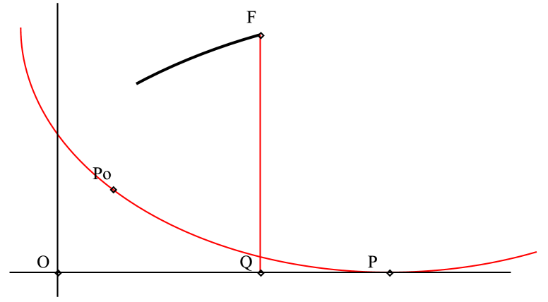
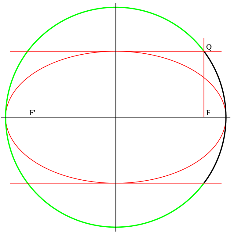
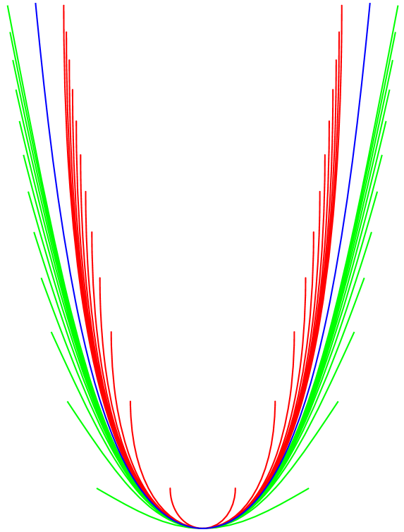
When a curve rolls, without slipping, on a fixed curve, each point of the rolling
curve traces another curve known as a roulette . In Figure 1 F = ( F 1 , F 2 ) 𝐹 subscript 𝐹 1 subscript 𝐹 2 F=(F_{1},F_{2}) C 𝐶 C F 1 subscript 𝐹 1 F_{1} Q 1 subscript 𝑄 1 Q_{1} P o subscript 𝑃 𝑜 P_{o} P 𝑃 P P 1 − Q 1 subscript 𝑃 1 subscript 𝑄 1 P_{1}-Q_{1} Q 𝑄 Q pedal curve of C 𝐶 C F 𝐹 F
The parametric description of the parabola , the ellipse and the hyperbola are given respectively by
α ( t ) = ( b sinh 2 ( t ) , 2 b sinh ( t ) ) , β ( t ) = ( a cos ( t ) , b sin ( t ) ) , γ ( t ) = ( a cosh ( t ) , b sinh ( t ) ) , 𝛼 𝑡 absent 𝑏 superscript 2 𝑡 2 𝑏 𝑡 𝛽 𝑡 absent 𝑎 𝑡 𝑏 𝑡 𝛾 𝑡 absent 𝑎 𝑡 𝑏 𝑡 \begin{array}[]{rl}\displaystyle\alpha(t)=&\left(b\sinh^{2}(t),2b\sinh(t)\right),\\[8.61108pt]
\displaystyle\beta(t)=&\Big{(}a\cos(t),b\sin(t)\Big{)},\\[8.61108pt]
\displaystyle\gamma(t)=&\Big{(}a\cosh(t),b\sinh(t)\Big{)},\end{array}
where a , b > 0 𝑎 𝑏
0 a,b>0 t ∈ [ t 1 , t 2 ] ⊂ ℝ 𝑡 subscript 𝑡 1 subscript 𝑡 2 ℝ t\in[t_{1},t_{2}]\subset\mathbb{R}
In Figure 1 F 𝐹 F P 𝑃 P
Figure 1: Roulette (left) and Parabola (right).
The arc length for the parabola from t 0 subscript 𝑡 0 t_{0}
s = ∫ t 0 t | α ′ ( u ) | 𝑑 u = b ( t + sinh ( t ) cosh ( t ) ) . 𝑠 superscript subscript subscript 𝑡 0 𝑡 superscript 𝛼 ′ 𝑢 differential-d 𝑢 𝑏 𝑡 𝑡 𝑡 s=\int_{t_{0}}^{t}|\alpha^{\prime}(u)|du=b(t+\sinh(t)\cosh(t)).
The length of the segment P Q ¯ ¯ 𝑃 𝑄 \overline{PQ} b sinh ( t ) cosh ( t ) 𝑏 𝑡 𝑡 b\sinh(t)\cosh(t)
g c ( t ) = s − b sinh ( t ) cosh ( t ) = b t . subscript 𝑔 𝑐 𝑡 𝑠 𝑏 𝑡 𝑡 𝑏 𝑡 g_{c}(t)=s-b\sinh(t)\cosh(t)=bt.
Computing f c ( t ) subscript 𝑓 𝑐 𝑡 f_{c}(t) F Q ¯ ¯ 𝐹 𝑄 \overline{FQ} catenary
A ( t ) = ( g c ( t ) , f c ( t ) ) = ( b t , b cosh ( t ) ) . 𝐴 𝑡 subscript 𝑔 𝑐 𝑡 subscript 𝑓 𝑐 𝑡 𝑏 𝑡 𝑏 𝑡 A(t)=(g_{c}(t),f_{c}(t))=\left(bt,b\cosh\left(t\right)\right).
Note also that
| A ′ ( t ) | = b cosh ( t ) , superscript 𝐴 ′ 𝑡 𝑏 𝑡 |A^{\prime}(t)|=b\cosh(t),
and the arc length is given by
ℓ c ( t ) = ∫ t 0 t | A ′ ( z ) | 𝑑 z = b sinh ( z ) | t 0 t . subscript ℓ 𝑐 𝑡 superscript subscript subscript 𝑡 0 𝑡 superscript 𝐴 ′ 𝑧 differential-d 𝑧 evaluated-at 𝑏 𝑧 subscript 𝑡 0 𝑡 \ell_{c}(t)=\int_{t_{0}}^{t}|A^{\prime}(z)|\,dz=b\sinh(z)\Big{|}_{t_{0}}^{t}.
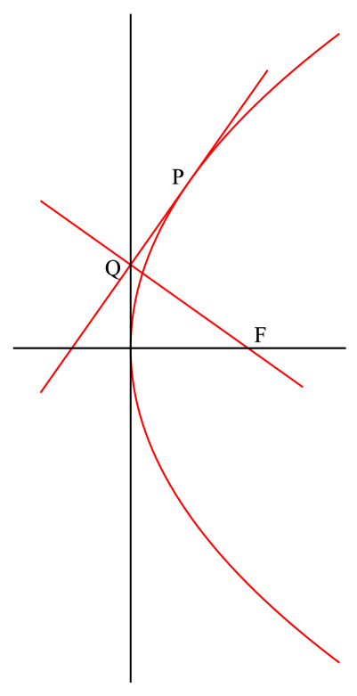
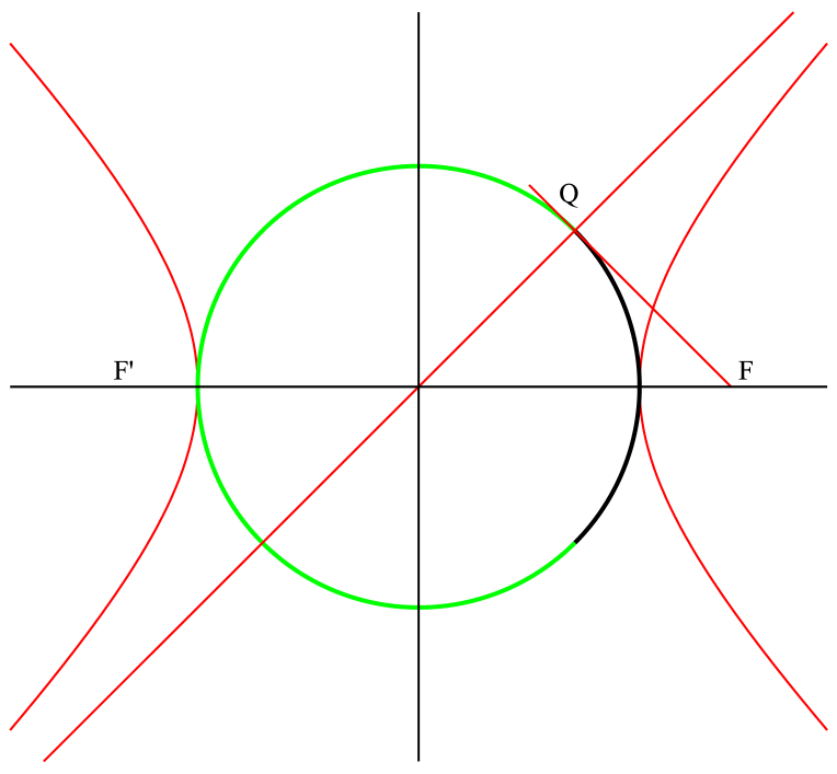
Figure 2: Ellipse (left) and Hyperbola (right).
For the ellipse, Figure 2 b < a 𝑏 𝑎 b<a c = a 2 − b 2 𝑐 superscript 𝑎 2 superscript 𝑏 2 c=\sqrt{a^{2}-b^{2}} t 0 subscript 𝑡 0 t_{0} t 𝑡 t
s = ∫ t 0 t | β ′ ( z ) | 𝑑 z = ∫ t 0 t a 2 − c 2 cos 2 ( z ) 𝑑 z . 𝑠 superscript subscript subscript 𝑡 0 𝑡 superscript 𝛽 ′ 𝑧 differential-d 𝑧 superscript subscript subscript 𝑡 0 𝑡 superscript 𝑎 2 superscript 𝑐 2 superscript 2 𝑧 differential-d 𝑧 s=\int_{t_{0}}^{t}|\beta^{\prime}(z)|dz=\int_{t_{0}}^{t}\sqrt{a^{2}-c^{2}\cos^{2}(z)}\,dz.
In this case two curves are generated. The first one corresponds to choosing the focus F 𝐹 F P Q ¯ ¯ 𝑃 𝑄 \overline{PQ}
g u 1 ( t ) = ∫ t 0 t a 2 − c 2 cos 2 ( z ) 𝑑 z − c sin ( t ) ( a − c cos ( t ) ) a 2 − c 2 cos 2 ( t ) . subscript superscript 𝑔 1 𝑢 𝑡 superscript subscript subscript 𝑡 0 𝑡 superscript 𝑎 2 superscript 𝑐 2 superscript 2 𝑧 differential-d 𝑧 𝑐 𝑡 𝑎 𝑐 𝑡 superscript 𝑎 2 superscript 𝑐 2 superscript 2 𝑡 g^{1}_{u}(t)=\int_{t_{0}}^{t}\sqrt{a^{2}-c^{2}\cos^{2}(z)}dz-\frac{c\sin(t)\left(a-c\cos(t)\right)}{\sqrt{a^{2}-c^{2}\cos^{2}(t)}}.
In addition, the ordinate is given by the length of the segment F Q ¯ ¯ 𝐹 𝑄 \overline{FQ}
f u 1 ( t ) = b ( a − c cos ( t ) ) a 2 − c 2 cos 2 ( t ) . subscript superscript 𝑓 1 𝑢 𝑡 𝑏 𝑎 𝑐 𝑡 superscript 𝑎 2 superscript 𝑐 2 superscript 2 𝑡 f^{1}_{u}(t)=\frac{b\left(a-c\cos(t)\right)}{\sqrt{a^{2}-c^{2}\cos^{2}(t)}}.
B 1 ( t ) = ( g u 1 ( t ) , f u 1 ( t ) ) subscript 𝐵 1 𝑡 subscript superscript 𝑔 1 𝑢 𝑡 subscript superscript 𝑓 1 𝑢 𝑡 B_{1}(t)=(g^{1}_{u}(t),f^{1}_{u}(t))
| B 1 ′ ( t ) | = a b a + c cos ( t ) , superscript subscript 𝐵 1 ′ 𝑡 𝑎 𝑏 𝑎 𝑐 𝑡 |B_{1}^{\prime}(t)|=\displaystyle\frac{ab}{a+c\cos(t)},
and the arc length is given by
ℓ u 1 ( t ) = ∫ t 0 t | B 1 ′ ( z ) | 𝑑 z = 2 a arctan ( a − c a + c tan ( z 2 ) ) | t 0 t . subscript superscript ℓ 1 𝑢 𝑡 superscript subscript subscript 𝑡 0 𝑡 superscript subscript 𝐵 1 ′ 𝑧 differential-d 𝑧 evaluated-at 2 𝑎 𝑎 𝑐 𝑎 𝑐 𝑧 2 subscript 𝑡 0 𝑡 {\ell^{1}_{u}}(t)=\int_{t_{0}}^{t}|B_{1}^{\prime}(z)|dz=\left.2a\arctan\left(\sqrt{\frac{a-c}{a+c}}\tan\left(\frac{z}{2}\right)\right)\right|_{t_{0}}^{t}.
In the same way, if we chooose the other focus F ′ superscript 𝐹 ′ F^{\prime} P Q ′ ¯ ¯ 𝑃 superscript 𝑄 ′ \overline{PQ^{\prime}}
g u 2 ( t ) = ∫ t 0 t a 2 − c 2 cos 2 ( z ) 𝑑 z − c sin ( t ) ( a + c cos ( t ) ) a 2 − c 2 cos 2 ( t ) , subscript superscript 𝑔 2 𝑢 𝑡 superscript subscript subscript 𝑡 0 𝑡 superscript 𝑎 2 superscript 𝑐 2 superscript 2 𝑧 differential-d 𝑧 𝑐 𝑡 𝑎 𝑐 𝑡 superscript 𝑎 2 superscript 𝑐 2 superscript 2 𝑡 g^{2}_{u}(t)=\int_{t_{0}}^{t}\sqrt{a^{2}-c^{2}\cos^{2}(z)}dz-\frac{c\sin(t)\left(a+c\cos(t)\right)}{\sqrt{a^{2}-c^{2}\cos^{2}(t)}},
and the ordinate is the length of the segment F ′ Q ′ ¯ ¯ superscript 𝐹 ′ superscript 𝑄 ′ \overline{F^{\prime}Q^{\prime}}
f u 2 ( t ) = b ( a + c cos ( t ) ) a 2 − c 2 cos 2 ( t ) . subscript superscript 𝑓 2 𝑢 𝑡 𝑏 𝑎 𝑐 𝑡 superscript 𝑎 2 superscript 𝑐 2 superscript 2 𝑡 f^{2}_{u}(t)=\frac{b\left(a+c\cos(t)\right)}{\sqrt{a^{2}-c^{2}\cos^{2}(t)}}.
B 2 ( t ) = ( g u 2 ( t ) , f u 2 ( t ) ) subscript 𝐵 2 𝑡 subscript superscript 𝑔 2 𝑢 𝑡 subscript superscript 𝑓 2 𝑢 𝑡 B_{2}(t)=(g^{2}_{u}(t),f^{2}_{u}(t)) F ′ superscript 𝐹 ′ F^{\prime}
| B 2 ′ ( t ) | = a b a − c cos ( t ) , superscript subscript 𝐵 2 ′ 𝑡 𝑎 𝑏 𝑎 𝑐 𝑡 |B_{2}^{\prime}(t)|=\displaystyle\frac{ab}{a-c\cos(t)},
and an arc length
ℓ u 2 ( t ) = ∫ t 0 t | B 2 ′ ( z ) | 𝑑 z = 2 a arctan ( a + c a − c tan ( z 2 ) ) | t 0 t . subscript superscript ℓ 2 𝑢 𝑡 superscript subscript subscript 𝑡 0 𝑡 superscript subscript 𝐵 2 ′ 𝑧 differential-d 𝑧 evaluated-at 2 𝑎 𝑎 𝑐 𝑎 𝑐 𝑧 2 subscript 𝑡 0 𝑡 {\ell^{2}_{u}}(t)=\int_{t_{0}}^{t}|B_{2}^{\prime}(z)|dz=\left.2a\arctan\left(\sqrt{\frac{a+c}{a-c}}\tan\left(\frac{z}{2}\right)\right)\right|_{t_{0}}^{t}.
Observe in particular that
arctan ( a + c a − c ) + arctan ( a − c a + c ) = π 2 𝑎 𝑐 𝑎 𝑐 𝑎 𝑐 𝑎 𝑐 𝜋 2 \arctan\left(\sqrt{\frac{a+c}{a-c}}\,\right)+\arctan\left(\sqrt{\frac{a-c}{a+c}}\,\right)=\frac{\pi}{2} t ∈ ( − π 2 , π 2 ) 𝑡 𝜋 2 𝜋 2 t\in(\frac{-\pi}{2},\frac{\pi}{2}) 2 π a 2 𝜋 𝑎 2\pi a
The roulette of the focus of an ellipse is called an undulary . It is clear that we do not need to consider both foci for an ellipse.
Specifically, if we consider the ellipse described by taking t ∈ [ − π , π ] 𝑡 𝜋 𝜋 t\in[-\pi,\pi] F 𝐹 F F 𝐹 F F ′ superscript 𝐹 ′ F^{\prime} t ∈ [ − π / 2 , π / 2 ] 𝑡 𝜋 2 𝜋 2 t\in[-\pi/2,\pi/2]
Consider now the case of the hyperbola, as shown Figure 2 c = a 2 + b 2 𝑐 superscript 𝑎 2 superscript 𝑏 2 c=\sqrt{a^{2}+b^{2}} t 0 subscript 𝑡 0 t_{0} t 𝑡 t
s = ∫ t 0 t | γ ′ ( z ) | 𝑑 z = ∫ t 0 t c 2 cosh 2 ( z ) − a 2 𝑑 z . 𝑠 superscript subscript subscript 𝑡 0 𝑡 superscript 𝛾 ′ 𝑧 differential-d 𝑧 superscript subscript subscript 𝑡 0 𝑡 superscript 𝑐 2 superscript 2 𝑧 superscript 𝑎 2 differential-d 𝑧 s=\displaystyle\int_{t_{0}}^{t}|\gamma^{\prime}(z)|dz=\displaystyle\int_{t_{0}}^{t}\sqrt{c^{2}\cosh^{2}(z)-a^{2}}\,dz.
For the first roulette we consider the focus F 𝐹 F P Q ¯ ¯ 𝑃 𝑄 \overline{PQ}
g n 1 ( t ) = ∫ t 0 t c 2 cosh 2 ( z ) − a 2 𝑑 z − c sinh ( t ) ( c cosh ( t ) − a ) c 2 cosh 2 ( t ) − a 2 , subscript superscript 𝑔 1 𝑛 𝑡 superscript subscript subscript 𝑡 0 𝑡 superscript 𝑐 2 superscript 2 𝑧 superscript 𝑎 2 differential-d 𝑧 𝑐 𝑡 𝑐 𝑡 𝑎 superscript 𝑐 2 superscript 2 𝑡 superscript 𝑎 2 g^{1}_{n}(t)=\int_{t_{0}}^{t}\sqrt{c^{2}\cosh^{2}(z)-a^{2}}\,dz-\frac{c\sinh(t)\left(c\cosh(t)-a\right)}{\sqrt{c^{2}\cosh^{2}(t)-a^{2}}},
whereas its ordinate is given by the length of F Q ¯ ¯ 𝐹 𝑄 \overline{FQ}
f n 1 ( t ) = b ( c cosh ( t ) − a ) c 2 cosh 2 ( t ) − a 2 . subscript superscript 𝑓 1 𝑛 𝑡 𝑏 𝑐 𝑡 𝑎 superscript 𝑐 2 superscript 2 𝑡 superscript 𝑎 2 f^{1}_{n}(t)=\frac{b\left(c\cosh(t)-a\right)}{\sqrt{c^{2}\cosh^{2}(t)-a^{2}}}.
C 1 ( t ) = ( g n 1 ( t ) , f n 1 ( t ) ) subscript 𝐶 1 𝑡 subscript superscript 𝑔 1 𝑛 𝑡 subscript superscript 𝑓 1 𝑛 𝑡 C_{1}(t)=(g^{1}_{n}(t),f^{1}_{n}(t)) F 𝐹 F
| C 1 ′ ( t ) | = a b c cosh ( t ) + a , superscript subscript 𝐶 1 ′ 𝑡 𝑎 𝑏 𝑐 𝑡 𝑎 |C_{1}^{\prime}(t)|=\displaystyle\frac{ab}{c\cosh(t)+a},
with arc length given by
ℓ 1 ( t ) = ∫ t 0 t | C 1 ′ ( z ) | d z = 2 a arctan ( c − a c + a tanh ( z 2 ) ) ] t 0 t . \ell_{1}(t)=\int_{t_{0}}^{t}|C_{1}^{\prime}(z)|dz=\left.2a\arctan\left(\sqrt{\frac{c-a}{c+a}}\tanh\left(\frac{z}{2}\right)\right)\right]_{t_{0}}^{t}.
In particular, the length of C 1 subscript 𝐶 1 C_{1} t ∈ ( − ∞ , ∞ ) 𝑡 t\in(-\infty,\infty) 4 a arctan ( c − a c + a ) . 4 𝑎 𝑐 𝑎 𝑐 𝑎 4a\arctan\left(\sqrt{\frac{c-a}{c+a}}\right).
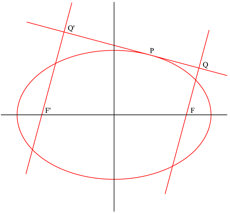
Figure 3: Roulettes B 1 subscript 𝐵 1 B_{1} B 2 subscript 𝐵 2 B_{2} C 1 subscript 𝐶 1 C_{1} C 2 subscript 𝐶 2 C_{2}
Taking the focus F ′ superscript 𝐹 ′ F^{\prime} P Q ′ ¯ ¯ 𝑃 superscript 𝑄 ′ \overline{PQ^{\prime}}
g n 2 ( t ) = ∫ t 0 t c 2 cosh 2 ( z ) − a 2 𝑑 z − c sinh ( t ) ( c cosh ( t ) + a ) c 2 cosh 2 ( t ) − a 2 , subscript superscript 𝑔 2 𝑛 𝑡 superscript subscript subscript 𝑡 0 𝑡 superscript 𝑐 2 superscript 2 𝑧 superscript 𝑎 2 differential-d 𝑧 𝑐 𝑡 𝑐 𝑡 𝑎 superscript 𝑐 2 superscript 2 𝑡 superscript 𝑎 2 g^{2}_{n}(t)=\int_{t_{0}}^{t}\sqrt{c^{2}\cosh^{2}(z)-a^{2}}\,dz-\frac{c\sinh(t)\left(c\cosh(t)+a\right)}{\sqrt{c^{2}\cosh^{2}(t)-a^{2}}},
and the ordinate is the length of the segment F ′ Q ′ ¯ ¯ superscript 𝐹 ′ superscript 𝑄 ′ \overline{F^{\prime}Q^{\prime}}
f n 2 ( t ) = b ( c cosh ( t ) + a ) c 2 cosh 2 ( t ) − a 2 . subscript superscript 𝑓 2 𝑛 𝑡 𝑏 𝑐 𝑡 𝑎 superscript 𝑐 2 superscript 2 𝑡 superscript 𝑎 2 f^{2}_{n}(t)=\frac{b\left(c\cosh(t)+a\right)}{\sqrt{c^{2}\cosh^{2}(t)-a^{2}}}.
C 2 ( t ) = ( g n 2 ( t ) , f n 2 ( t ) ) subscript 𝐶 2 𝑡 subscript superscript 𝑔 2 𝑛 𝑡 subscript superscript 𝑓 2 𝑛 𝑡 C_{2}(t)=(g^{2}_{n}(t),f^{2}_{n}(t)) F ′ superscript 𝐹 ′ F^{\prime}
| C 2 ′ ( t ) | = a b c cosh ( t ) − a , superscript subscript 𝐶 2 ′ 𝑡 𝑎 𝑏 𝑐 𝑡 𝑎 |C_{2}^{\prime}(t)|=\displaystyle\frac{ab}{c\cosh(t)-a},
and the arc length is given by
ℓ 2 ( t ) = ∫ t 0 t | C 2 ′ ( z ) | d z = 2 a arctan ( c + a c − a tanh ( z 2 ) ) ] t 0 t . {\ell_{2}}(t)=\int_{t_{0}}^{t}|C_{2}^{\prime}(z)|dz=\left.2a\arctan\left(\sqrt{\frac{c+a}{c-a}}\tanh\left(\frac{z}{2}\right)\right)\right]_{t_{0}}^{t}.
The sum of the length of the two branches of the curves for t ∈ ( − ∞ , ∞ ) 𝑡 t\in(-\infty,\infty) 2 π a 2 𝜋 𝑎 2\pi a nodary .
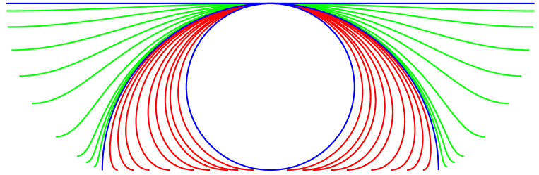
In Figure 3 B 1 subscript 𝐵 1 B_{1} C 1 subscript 𝐶 1 C_{1} B 2 subscript 𝐵 2 B_{2} C 2 subscript 𝐶 2 C_{2}
Figure 4: Pedal curves of the ellipse and the hyperbola. Left: arc of the circle (black), whose length coincides
with the length of the curve B 1 subscript 𝐵 1 B_{1} B 2 subscript 𝐵 2 B_{2} C 1 subscript 𝐶 1 C_{1} C 2 subscript 𝐶 2 C_{2}
In Figure 4 C 1 subscript 𝐶 1 C_{1} x = arctan ( c − a c + a ) , 𝑥 𝑐 𝑎 𝑐 𝑎 x=\arctan\left(\sqrt{\frac{c-a}{c+a}}\,\right),
sin ( 2 x ) = b c cos ( 2 x ) = a c , formulae-sequence 2 𝑥 𝑏 𝑐 2 𝑥 𝑎 𝑐 \sin(2x)=\frac{b}{c}\hskip 56.9055pt\cos(2x)=\frac{a}{c},
and so
4 a arctan ( c − a c + a ) = 2 a arctan ( b a ) . 4 𝑎 𝑐 𝑎 𝑐 𝑎 2 𝑎 𝑏 𝑎 4a\arctan\left(\sqrt{\frac{c-a}{c+a}}\,\right)=2a\arctan\left(\frac{b}{a}\right).
That is, the length of the curve C 1 subscript 𝐶 1 C_{1} 4
Figure 5: Family of roulettes B 1 ∪ B 2 subscript 𝐵 1 subscript 𝐵 2 B_{1}\cup B_{2} C 1 ∪ C 2 subscript 𝐶 1 subscript 𝐶 2 C_{1}\cup C_{2} 2 π a 2 𝜋 𝑎 2\pi a
In Figure 5 2 π a 2 𝜋 𝑎 2\pi a a 𝑎 a B 𝐵 B b = a 𝑏 𝑎 b=a b = a 𝑏 𝑎 b=a b = 0 𝑏 0 b=0 2 a 2 𝑎 2a C 𝐶 C b = 0 𝑏 0 b=0 b = ∞ 𝑏 b=\infty a 𝑎 a
Figure 6: Left: Location of the roulettes in Figure 5 B 1 subscript 𝐵 1 B_{1} C 1 subscript 𝐶 1 C_{1}
In Figure 6 5 a 𝑎 a b = ∞ 𝑏 b=\infty 6 B 1 subscript 𝐵 1 B_{1} C 1 subscript 𝐶 1 C_{1} a 𝑎 a a 𝑎 a
3 The Delaunay Surfaces
In this section we study Delaunay surfaces and derive analytical expressions for their most
important differential geometric properties. The Delaunay surfaces are surfaces of revolution and therefore the key to their properties
lie in their meridians, which here are the roulettes of the foci of the conics discussed in the previous section.
The Delaunay surfaces are thus the surfaces of revolution generated by the curves A ( t ) 𝐴 𝑡 A(t) B 1 ( t ) subscript 𝐵 1 𝑡 B_{1}(t) B 2 ( t ) subscript 𝐵 2 𝑡 B_{2}(t) C 1 ( t ) subscript 𝐶 1 𝑡 C_{1}(t) C 2 ( t ) subscript 𝐶 2 𝑡 C_{2}(t)
Catenoid: x x x x x x x x x x x x x x ( t , v ) = ( f c ( t ) cos ( v ) , f c ( t ) sin ( v ) , g c ( t ) ) , x x x x x x x x x x x x x x 𝑡 𝑣 subscript 𝑓 𝑐 𝑡 𝑣 subscript 𝑓 𝑐 𝑡 𝑣 subscript 𝑔 𝑐 𝑡 \kern-0.33005pt\hbox{$x$}\kern-5.71527pt\kern 0.11002pt\hbox{$x$}\kern-5.71527pt\kern 0.11002pt\hbox{$x$}\kern-5.71527pt\kern 0.11002pt\hbox{$x$}\kern-5.71527pt\kern 0.11002pt\hbox{$x$}\kern-5.71527pt\kern 0.11002pt\hbox{$x$}\kern-5.71527pt\kern 0.11002pt\hbox{$x$}\kern-5.71527pt\kern-0.54993pt\raise 0.15pt\hbox{$x$}\kern-5.71527pt\kern 0.11002pt\raise 0.15pt\hbox{$x$}\kern-5.71527pt\kern 0.11002pt\raise 0.15pt\hbox{$x$}\kern-5.71527pt\kern 0.11002pt\raise-0.15pt\hbox{$x$}\kern-5.71527pt\kern 0.11002pt\raise-0.15pt\hbox{$x$}\kern-5.71527pt\kern-0.22003pt\hbox{$x$}\kern-5.71527pt\raise-0.15pt\hbox{$x$}(t,v)=\Big{(}f_{c}(t)\cos(v),f_{c}(t)\sin(v),g_{c}(t)\Big{)}, 7
x x x x x x x x x x x x x x t = ( b sinh ( t ) cos ( v ) , b sinh ( t ) sin ( v ) , b ) , x x x x x x x x x x x x x x v = ( − b cosh ( t ) sin ( v ) , b cosh ( t ) cos ( v ) , 0 ) . subscript x x x x x x x x x x x x x x 𝑡 absent 𝑏 𝑡 𝑣 𝑏 𝑡 𝑣 𝑏 subscript x x x x x x x x x x x x x x 𝑣 absent 𝑏 𝑡 𝑣 𝑏 𝑡 𝑣 0 \begin{array}[]{rl}{\kern-0.33005pt\hbox{$x$}\kern-5.71527pt\kern 0.11002pt\hbox{$x$}\kern-5.71527pt\kern 0.11002pt\hbox{$x$}\kern-5.71527pt\kern 0.11002pt\hbox{$x$}\kern-5.71527pt\kern 0.11002pt\hbox{$x$}\kern-5.71527pt\kern 0.11002pt\hbox{$x$}\kern-5.71527pt\kern 0.11002pt\hbox{$x$}\kern-5.71527pt\kern-0.54993pt\raise 0.15pt\hbox{$x$}\kern-5.71527pt\kern 0.11002pt\raise 0.15pt\hbox{$x$}\kern-5.71527pt\kern 0.11002pt\raise 0.15pt\hbox{$x$}\kern-5.71527pt\kern 0.11002pt\raise-0.15pt\hbox{$x$}\kern-5.71527pt\kern 0.11002pt\raise-0.15pt\hbox{$x$}\kern-5.71527pt\kern-0.22003pt\hbox{$x$}\kern-5.71527pt\raise-0.15pt\hbox{$x$}}_{t}=&\left(b\sinh(t)\cos(v),b\sinh(t)\sin(v),b\right),\\[4.30554pt]
{\kern-0.33005pt\hbox{$x$}\kern-5.71527pt\kern 0.11002pt\hbox{$x$}\kern-5.71527pt\kern 0.11002pt\hbox{$x$}\kern-5.71527pt\kern 0.11002pt\hbox{$x$}\kern-5.71527pt\kern 0.11002pt\hbox{$x$}\kern-5.71527pt\kern 0.11002pt\hbox{$x$}\kern-5.71527pt\kern 0.11002pt\hbox{$x$}\kern-5.71527pt\kern-0.54993pt\raise 0.15pt\hbox{$x$}\kern-5.71527pt\kern 0.11002pt\raise 0.15pt\hbox{$x$}\kern-5.71527pt\kern 0.11002pt\raise 0.15pt\hbox{$x$}\kern-5.71527pt\kern 0.11002pt\raise-0.15pt\hbox{$x$}\kern-5.71527pt\kern 0.11002pt\raise-0.15pt\hbox{$x$}\kern-5.71527pt\kern-0.22003pt\hbox{$x$}\kern-5.71527pt\raise-0.15pt\hbox{$x$}}_{v}=&\left(-b\cosh(t)\sin(v),b\cosh(t)\cos(v),0\right).\end{array}
The unit normal vector at ( t , v ) 𝑡 𝑣 (t,v)
n n n n n n n n n n n n n n c ( t , v ) = ( − cos ( v ) cosh ( t ) , − sin ( v ) cosh ( t ) , tanh ( t ) ) . subscript n n n n n n n n n n n n n n 𝑐 𝑡 𝑣 𝑣 𝑡 𝑣 𝑡 𝑡 {\kern-0.33005pt\hbox{$n$}\kern-6.00235pt\kern 0.11002pt\hbox{$n$}\kern-6.00235pt\kern 0.11002pt\hbox{$n$}\kern-6.00235pt\kern 0.11002pt\hbox{$n$}\kern-6.00235pt\kern 0.11002pt\hbox{$n$}\kern-6.00235pt\kern 0.11002pt\hbox{$n$}\kern-6.00235pt\kern 0.11002pt\hbox{$n$}\kern-6.00235pt\kern-0.54993pt\raise 0.15pt\hbox{$n$}\kern-6.00235pt\kern 0.11002pt\raise 0.15pt\hbox{$n$}\kern-6.00235pt\kern 0.11002pt\raise 0.15pt\hbox{$n$}\kern-6.00235pt\kern 0.11002pt\raise-0.15pt\hbox{$n$}\kern-6.00235pt\kern 0.11002pt\raise-0.15pt\hbox{$n$}\kern-6.00235pt\kern-0.22003pt\hbox{$n$}\kern-6.00235pt\raise-0.15pt\hbox{$n$}}_{c}(t,v)=\left(-\frac{\cos(v)}{\cosh(t)},-\frac{\sin(v)}{\cosh(t)},\tanh(t)\right).
The non–vanishing coeficients of the first and the second fundamental form, and the principal curvatures, the mean curvature
and the Gaussian curvature are,
E = b 2 cosh 2 ( t ) , G = b 2 cosh 2 ( t ) , L = − b , N = b , k 1 = − 1 b cosh 2 ( t ) , k 2 = 1 b cosh 2 ( t ) , H = 0 , K = − 1 b 2 cosh 4 ( t ) . 𝐸 absent superscript 𝑏 2 superscript 2 𝑡 𝐺 absent superscript 𝑏 2 superscript 2 𝑡 𝐿 absent 𝑏 𝑁 absent 𝑏 subscript 𝑘 1 absent 1 𝑏 superscript 2 𝑡 subscript 𝑘 2 absent 1 𝑏 superscript 2 𝑡 𝐻 absent 0 𝐾 absent 1 superscript 𝑏 2 superscript 4 𝑡 \begin{array}[]{rlrlrlrl}E=&\displaystyle b^{2}\cosh^{2}(t),&G=&\displaystyle b^{2}\cosh^{2}(t),&L=&\displaystyle-b,&N=&\displaystyle b,\\[4.30554pt]
k_{1}=&\displaystyle\frac{-1}{b\cosh^{2}(t)},&k_{2}=&\displaystyle\frac{1}{b\cosh^{2}(t)},&H=&\displaystyle 0,&K=&\displaystyle\frac{-1}{b^{2}\cosh^{4}(t)}.\end{array}
Figure 7: The catenoid.
The geodesic curvature of a parallel is
k g = sinh ( t ) b cosh 2 ( t ) , subscript 𝑘 𝑔 𝑡 𝑏 superscript 2 𝑡 k_{g}=\frac{\sinh(t)}{b\cosh^{2}(t)},
and the total curvature of the catenoid is
∫ x x x x x x x x x x x x x x K 𝑑 σ = − ( v 2 − v 1 ) tanh ( t ) | t 1 t 2 . subscript x x x x x x x x x x x x x x 𝐾 differential-d 𝜎 evaluated-at subscript 𝑣 2 subscript 𝑣 1 𝑡 subscript 𝑡 1 subscript 𝑡 2 \int_{\kern-0.23103pt\hbox{$x$}\kern-4.00069pt\kern 0.07701pt\hbox{$x$}\kern-4.00069pt\kern 0.07701pt\hbox{$x$}\kern-4.00069pt\kern 0.07701pt\hbox{$x$}\kern-4.00069pt\kern 0.07701pt\hbox{$x$}\kern-4.00069pt\kern 0.07701pt\hbox{$x$}\kern-4.00069pt\kern 0.07701pt\hbox{$x$}\kern-4.00069pt\kern-0.38495pt\raise 0.105pt\hbox{$x$}\kern-4.00069pt\kern 0.07701pt\raise 0.105pt\hbox{$x$}\kern-4.00069pt\kern 0.07701pt\raise 0.105pt\hbox{$x$}\kern-4.00069pt\kern 0.07701pt\raise-0.105pt\hbox{$x$}\kern-4.00069pt\kern 0.07701pt\raise-0.105pt\hbox{$x$}\kern-4.00069pt\kern-0.15402pt\hbox{$x$}\kern-4.00069pt\raise-0.105pt\hbox{$x$}}Kd\sigma=-(v_{2}-v_{1})\tanh(t)\Big{|}_{t_{1}}^{t_{2}}.
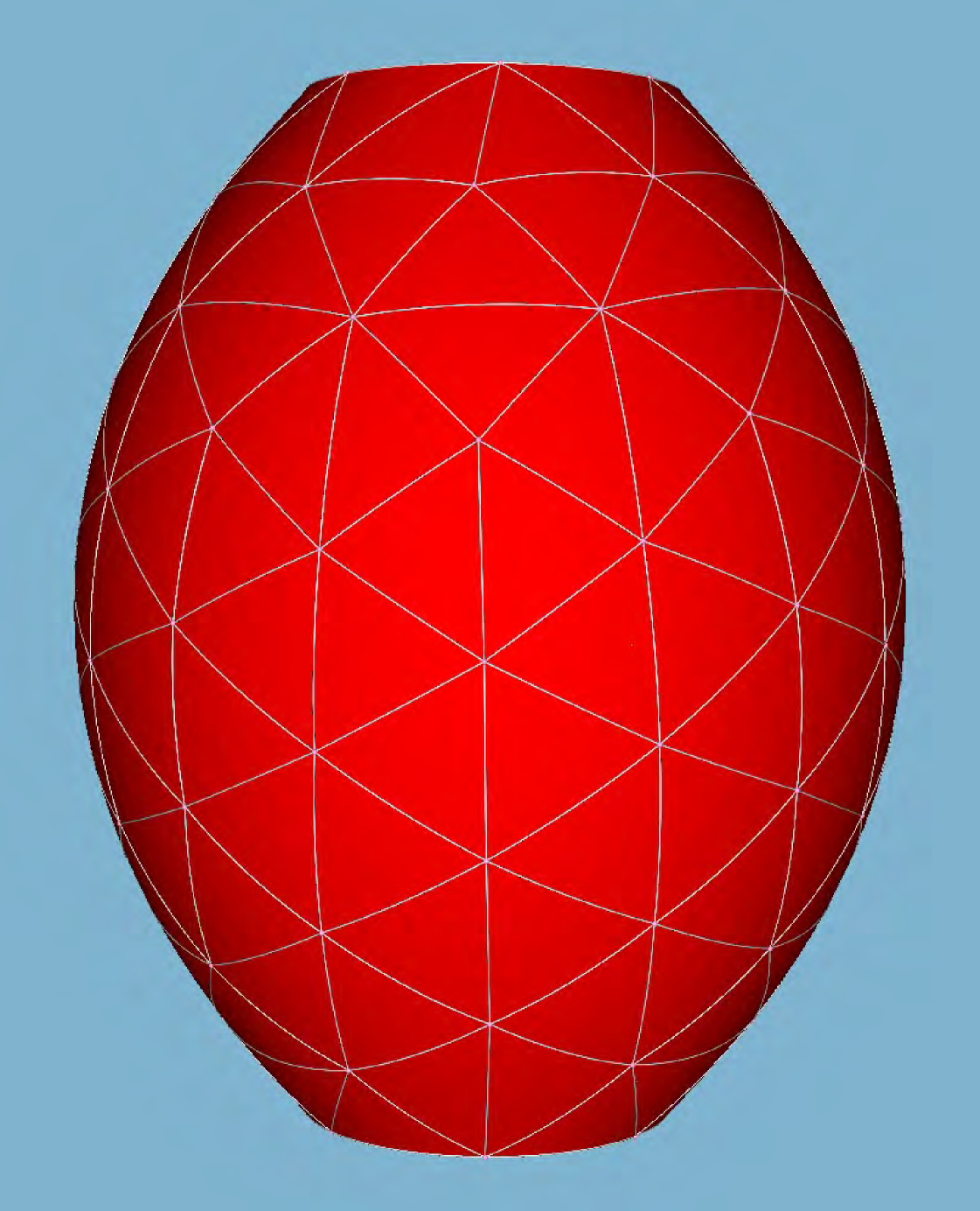
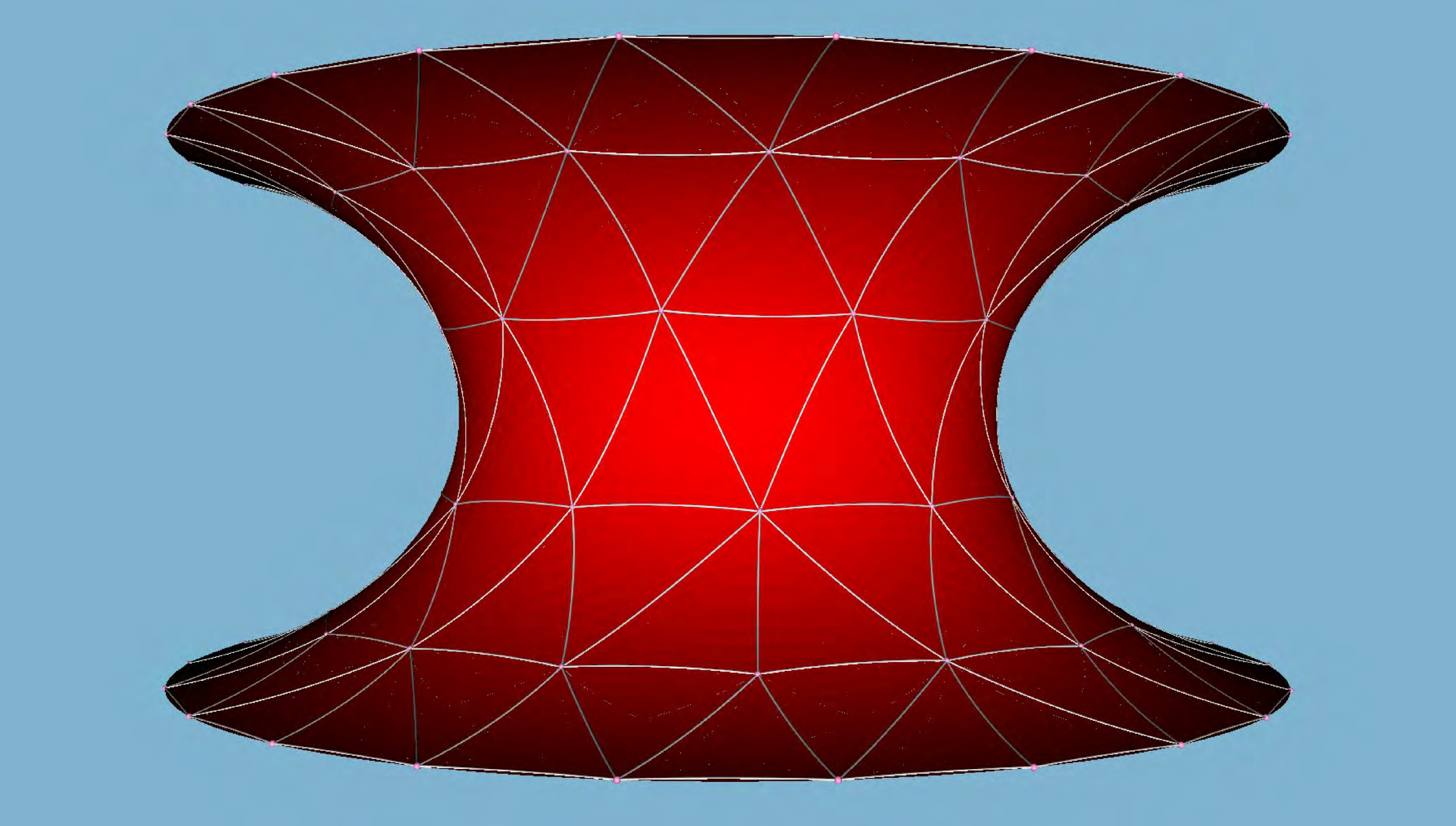
Unduloid: y y y y y y y y y y y y y y ( t , v ) = ( f u 1 ( t ) cos ( v ) , f u 1 ( t ) sin ( v ) , g u 1 ( t ) ) , y y y y y y y y y y y y y y 𝑡 𝑣 superscript subscript 𝑓 𝑢 1 𝑡 𝑣 superscript subscript 𝑓 𝑢 1 𝑡 𝑣 superscript subscript 𝑔 𝑢 1 𝑡 {\kern-0.33005pt\hbox{$y$}\kern-5.2616pt\kern 0.11002pt\hbox{$y$}\kern-5.2616pt\kern 0.11002pt\hbox{$y$}\kern-5.2616pt\kern 0.11002pt\hbox{$y$}\kern-5.2616pt\kern 0.11002pt\hbox{$y$}\kern-5.2616pt\kern 0.11002pt\hbox{$y$}\kern-5.2616pt\kern 0.11002pt\hbox{$y$}\kern-5.2616pt\kern-0.54993pt\raise 0.15pt\hbox{$y$}\kern-5.2616pt\kern 0.11002pt\raise 0.15pt\hbox{$y$}\kern-5.2616pt\kern 0.11002pt\raise 0.15pt\hbox{$y$}\kern-5.2616pt\kern 0.11002pt\raise-0.15pt\hbox{$y$}\kern-5.2616pt\kern 0.11002pt\raise-0.15pt\hbox{$y$}\kern-5.2616pt\kern-0.22003pt\hbox{$y$}\kern-5.2616pt\raise-0.15pt\hbox{$y$}}(t,v)=\Big{(}f_{u}^{1}(t)\cos(v),f_{u}^{1}(t)\sin(v),g_{u}^{1}(t)\Big{)}, 8
h u ( t ) = a b a 2 − c 2 cos 2 ( t ) ( a + c cos ( t ) ) subscript ℎ 𝑢 𝑡 𝑎 𝑏 superscript 𝑎 2 superscript 𝑐 2 superscript 2 𝑡 𝑎 𝑐 𝑡 h_{u}(t)=\frac{ab}{\sqrt{a^{2}-c^{2}\cos^{2}(t)}\left(a+c\cos(t)\right)}
it follows that
y y y y y y y y y y y y y y t = ( c sin ( t ) h u ( t ) cos ( v ) , c sin ( t ) h u ( t ) sin ( v ) , b h u ( t ) ) , y y y y y y y y y y y y y y v = ( − f u 1 ( t ) sin ( v ) , f u 1 ( t ) cos ( v ) , 0 ) . subscript y y y y y y y y y y y y y y 𝑡 absent 𝑐 𝑡 subscript ℎ 𝑢 𝑡 𝑣 𝑐 𝑡 subscript ℎ 𝑢 𝑡 𝑣 𝑏 subscript ℎ 𝑢 𝑡 subscript y y y y y y y y y y y y y y 𝑣 absent superscript subscript 𝑓 𝑢 1 𝑡 𝑣 superscript subscript 𝑓 𝑢 1 𝑡 𝑣 0 \begin{array}[]{rl}{\kern-0.33005pt\hbox{$y$}\kern-5.2616pt\kern 0.11002pt\hbox{$y$}\kern-5.2616pt\kern 0.11002pt\hbox{$y$}\kern-5.2616pt\kern 0.11002pt\hbox{$y$}\kern-5.2616pt\kern 0.11002pt\hbox{$y$}\kern-5.2616pt\kern 0.11002pt\hbox{$y$}\kern-5.2616pt\kern 0.11002pt\hbox{$y$}\kern-5.2616pt\kern-0.54993pt\raise 0.15pt\hbox{$y$}\kern-5.2616pt\kern 0.11002pt\raise 0.15pt\hbox{$y$}\kern-5.2616pt\kern 0.11002pt\raise 0.15pt\hbox{$y$}\kern-5.2616pt\kern 0.11002pt\raise-0.15pt\hbox{$y$}\kern-5.2616pt\kern 0.11002pt\raise-0.15pt\hbox{$y$}\kern-5.2616pt\kern-0.22003pt\hbox{$y$}\kern-5.2616pt\raise-0.15pt\hbox{$y$}}_{t}=&\left(c\sin(t)h_{u}(t)\cos(v),c\sin(t)h_{u}(t)\sin(v),bh_{u}(t)\right),\\[4.30554pt]
{\kern-0.33005pt\hbox{$y$}\kern-5.2616pt\kern 0.11002pt\hbox{$y$}\kern-5.2616pt\kern 0.11002pt\hbox{$y$}\kern-5.2616pt\kern 0.11002pt\hbox{$y$}\kern-5.2616pt\kern 0.11002pt\hbox{$y$}\kern-5.2616pt\kern 0.11002pt\hbox{$y$}\kern-5.2616pt\kern 0.11002pt\hbox{$y$}\kern-5.2616pt\kern-0.54993pt\raise 0.15pt\hbox{$y$}\kern-5.2616pt\kern 0.11002pt\raise 0.15pt\hbox{$y$}\kern-5.2616pt\kern 0.11002pt\raise 0.15pt\hbox{$y$}\kern-5.2616pt\kern 0.11002pt\raise-0.15pt\hbox{$y$}\kern-5.2616pt\kern 0.11002pt\raise-0.15pt\hbox{$y$}\kern-5.2616pt\kern-0.22003pt\hbox{$y$}\kern-5.2616pt\raise-0.15pt\hbox{$y$}}_{v}=&\left(-f_{u}^{1}(t)\sin(v),f_{u}^{1}(t)\cos(v),0\right).\end{array}
The unit normal vector at ( t , v ) 𝑡 𝑣 (t,v)
n n n n n n n n n n n n n n u ( t , v ) = ( − b cos ( v ) a 2 − c 2 cos 2 ( t ) , − b sin ( v ) a 2 − c 2 cos 2 ( t ) , c sin ( t ) a 2 − c 2 cos 2 ( t ) ) . subscript n n n n n n n n n n n n n n 𝑢 𝑡 𝑣 𝑏 𝑣 superscript 𝑎 2 superscript 𝑐 2 superscript 2 𝑡 𝑏 𝑣 superscript 𝑎 2 superscript 𝑐 2 superscript 2 𝑡 𝑐 𝑡 superscript 𝑎 2 superscript 𝑐 2 superscript 2 𝑡 {\kern-0.33005pt\hbox{$n$}\kern-6.00235pt\kern 0.11002pt\hbox{$n$}\kern-6.00235pt\kern 0.11002pt\hbox{$n$}\kern-6.00235pt\kern 0.11002pt\hbox{$n$}\kern-6.00235pt\kern 0.11002pt\hbox{$n$}\kern-6.00235pt\kern 0.11002pt\hbox{$n$}\kern-6.00235pt\kern 0.11002pt\hbox{$n$}\kern-6.00235pt\kern-0.54993pt\raise 0.15pt\hbox{$n$}\kern-6.00235pt\kern 0.11002pt\raise 0.15pt\hbox{$n$}\kern-6.00235pt\kern 0.11002pt\raise 0.15pt\hbox{$n$}\kern-6.00235pt\kern 0.11002pt\raise-0.15pt\hbox{$n$}\kern-6.00235pt\kern 0.11002pt\raise-0.15pt\hbox{$n$}\kern-6.00235pt\kern-0.22003pt\hbox{$n$}\kern-6.00235pt\raise-0.15pt\hbox{$n$}}_{u}(t,v)=\left(\frac{-b\cos(v)}{\sqrt{a^{2}-c^{2}\cos^{2}(t)}},\frac{-b\sin(v)}{\sqrt{a^{2}-c^{2}\cos^{2}(t)}},\frac{c\sin(t)}{\sqrt{a^{2}-c^{2}\cos^{2}(t)}}\right).
E = a 2 b 2 ( a + c cos ( t ) ) 2 , G = b 2 ( a − c cos ( t ) ) ( a + c cos ( t ) ) , L = − a b 2 c cos ( t ) ( a 2 − c 2 cos 2 ( t ) ) ( a + c cos ( t ) ) , N = b 2 a + c cos ( t ) , k 1 = − c cos ( t ) a ( a − c cos ( t ) ) , k 2 = 1 a − c cos ( t ) , H = 1 2 a , K = − c cos ( t ) a ( a − c cos ( t ) ) 2 . 𝐸 absent superscript 𝑎 2 superscript 𝑏 2 superscript 𝑎 𝑐 𝑡 2 𝐺 absent superscript 𝑏 2 𝑎 𝑐 𝑡 𝑎 𝑐 𝑡 𝐿 absent 𝑎 superscript 𝑏 2 𝑐 𝑡 superscript 𝑎 2 superscript 𝑐 2 superscript 2 𝑡 𝑎 𝑐 𝑡 𝑁 absent superscript 𝑏 2 𝑎 𝑐 𝑡 subscript 𝑘 1 absent 𝑐 𝑡 𝑎 𝑎 𝑐 𝑡 subscript 𝑘 2 absent 1 𝑎 𝑐 𝑡 𝐻 absent 1 2 𝑎 𝐾 absent 𝑐 𝑡 𝑎 superscript 𝑎 𝑐 𝑡 2 \begin{array}[]{rlrl }E=&\displaystyle\frac{a^{2}b^{2}}{\left(a+c\cos(t)\right)^{2}},&\hskip 28.45274ptG=&\displaystyle\frac{b^{2}\left(a-c\cos(t)\right)}{\left(a+c\cos(t)\right)},\\[12.91663pt]
L=&\displaystyle\displaystyle\frac{-ab^{2}c\cos(t)}{\left(a^{2}-c^{2}\cos^{2}(t)\right)\left(a+c\cos(t)\right)},&N=&\displaystyle\frac{b^{2}}{a+c\cos(t)},\\[12.91663pt]
k_{1}=&\displaystyle\frac{-c\cos(t)}{a(a-c\cos(t))},&k_{2}=&\displaystyle\frac{1}{a-c\cos(t)},\\[12.91663pt]
H=&\displaystyle\frac{1}{2a},&K=&\displaystyle\frac{-c\cos(t)}{\displaystyle a\left(a-c\cos(t)\right)^{2}}.\end{array}
The geodesic curvature of a parallel is
k g = − c sin ( t ) b ( a − c cos ( t ) ) , subscript 𝑘 𝑔 𝑐 𝑡 𝑏 𝑎 𝑐 𝑡 k_{g}=\frac{-c\sin(t)}{b\big{(}a-c\cos(t)\big{)}},
and the total curvature is
∫ y y y y y y y y y y y y y y K 𝑑 σ = − c ( v 2 − v 1 ) sin ( t ) a 2 − c 2 cos 2 ( t ) | t 1 t 2 . subscript y y y y y y y y y y y y y y 𝐾 differential-d 𝜎 evaluated-at 𝑐 subscript 𝑣 2 subscript 𝑣 1 𝑡 superscript 𝑎 2 superscript 𝑐 2 superscript 2 𝑡 subscript 𝑡 1 subscript 𝑡 2 \int_{\kern-0.23103pt\hbox{$y$}\kern-3.6831pt\kern 0.07701pt\hbox{$y$}\kern-3.6831pt\kern 0.07701pt\hbox{$y$}\kern-3.6831pt\kern 0.07701pt\hbox{$y$}\kern-3.6831pt\kern 0.07701pt\hbox{$y$}\kern-3.6831pt\kern 0.07701pt\hbox{$y$}\kern-3.6831pt\kern 0.07701pt\hbox{$y$}\kern-3.6831pt\kern-0.38495pt\raise 0.105pt\hbox{$y$}\kern-3.6831pt\kern 0.07701pt\raise 0.105pt\hbox{$y$}\kern-3.6831pt\kern 0.07701pt\raise 0.105pt\hbox{$y$}\kern-3.6831pt\kern 0.07701pt\raise-0.105pt\hbox{$y$}\kern-3.6831pt\kern 0.07701pt\raise-0.105pt\hbox{$y$}\kern-3.6831pt\kern-0.15402pt\hbox{$y$}\kern-3.6831pt\raise-0.105pt\hbox{$y$}}Kd\sigma=\left.-c(v_{2}-v_{1})\frac{\sin(t)}{\sqrt{a^{2}-c^{2}\cos^{2}(t)}}\right|_{t_{1}}^{t_{2}}.
Figure 8: Unduloids generated by the revolution of B 1 subscript 𝐵 1 B_{1} B 2 subscript 𝐵 2 B_{2}
Clearly one could do the same calculation for the surface generated by B 2 subscript 𝐵 2 B_{2} 8 t 𝑡 t 2 π 2 𝜋 2\pi t 𝑡 t
We must, however, consider both parts C 1 subscript 𝐶 1 C_{1} C 2 subscript 𝐶 2 C_{2} I R I R \rm I\!R
Nodoid1: z z z z z z z z z z z z z z 1 ( t , v ) = ( f n 1 ( t ) cos ( v ) , f n 1 ( t ) sin ( v ) , g n 1 ( t ) ) , subscript z z z z z z z z z z z z z z 1 𝑡 𝑣 superscript subscript 𝑓 𝑛 1 𝑡 𝑣 superscript subscript 𝑓 𝑛 1 𝑡 𝑣 superscript subscript 𝑔 𝑛 1 𝑡 \kern-0.33005pt\hbox{$z$}\kern-5.0903pt\kern 0.11002pt\hbox{$z$}\kern-5.0903pt\kern 0.11002pt\hbox{$z$}\kern-5.0903pt\kern 0.11002pt\hbox{$z$}\kern-5.0903pt\kern 0.11002pt\hbox{$z$}\kern-5.0903pt\kern 0.11002pt\hbox{$z$}\kern-5.0903pt\kern 0.11002pt\hbox{$z$}\kern-5.0903pt\kern-0.54993pt\raise 0.15pt\hbox{$z$}\kern-5.0903pt\kern 0.11002pt\raise 0.15pt\hbox{$z$}\kern-5.0903pt\kern 0.11002pt\raise 0.15pt\hbox{$z$}\kern-5.0903pt\kern 0.11002pt\raise-0.15pt\hbox{$z$}\kern-5.0903pt\kern 0.11002pt\raise-0.15pt\hbox{$z$}\kern-5.0903pt\kern-0.22003pt\hbox{$z$}\kern-5.0903pt\raise-0.15pt\hbox{$z$}_{1}(t,v)=\Big{(}f_{n}^{1}(t)\cos(v),f_{n}^{1}(t)\sin(v),g_{n}^{1}(t)\Big{)}, 9
h 1 ( t ) = a b c 2 cosh 2 ( t ) − a 2 ( c cosh ( t ) + a ) subscript ℎ 1 𝑡 𝑎 𝑏 superscript 𝑐 2 superscript 2 𝑡 superscript 𝑎 2 𝑐 𝑡 𝑎 h_{1}(t)=\frac{ab}{\sqrt{c^{2}\cosh^{2}(t)-a^{2}}\left(c\cosh(t)+a\right)}
from which it follows that
( z z z z z z z z z z z z z z 1 ) t = ( c sinh ( t ) h 1 ( t ) cos ( v ) , c sinh ( t ) h 1 ( t ) sin ( v ) , b h 1 ( t ) ) , ( z z z z z z z z z z z z z z 1 ) v = ( − f n 1 ( t ) sin ( v ) , f n 1 ( t ) cos ( v ) , 0 ) . subscript subscript z z z z z z z z z z z z z z 1 𝑡 absent 𝑐 𝑡 subscript ℎ 1 𝑡 𝑣 𝑐 𝑡 subscript ℎ 1 𝑡 𝑣 𝑏 subscript ℎ 1 𝑡 subscript subscript z z z z z z z z z z z z z z 1 𝑣 absent superscript subscript 𝑓 𝑛 1 𝑡 𝑣 superscript subscript 𝑓 𝑛 1 𝑡 𝑣 0 \begin{array}[]{rl}({\kern-0.33005pt\hbox{$z$}\kern-5.0903pt\kern 0.11002pt\hbox{$z$}\kern-5.0903pt\kern 0.11002pt\hbox{$z$}\kern-5.0903pt\kern 0.11002pt\hbox{$z$}\kern-5.0903pt\kern 0.11002pt\hbox{$z$}\kern-5.0903pt\kern 0.11002pt\hbox{$z$}\kern-5.0903pt\kern 0.11002pt\hbox{$z$}\kern-5.0903pt\kern-0.54993pt\raise 0.15pt\hbox{$z$}\kern-5.0903pt\kern 0.11002pt\raise 0.15pt\hbox{$z$}\kern-5.0903pt\kern 0.11002pt\raise 0.15pt\hbox{$z$}\kern-5.0903pt\kern 0.11002pt\raise-0.15pt\hbox{$z$}\kern-5.0903pt\kern 0.11002pt\raise-0.15pt\hbox{$z$}\kern-5.0903pt\kern-0.22003pt\hbox{$z$}\kern-5.0903pt\raise-0.15pt\hbox{$z$}}_{1})_{t}=&\Big{(}c\sinh(t)h_{1}(t)\cos(v),c\sinh(t)h_{1}(t)\sin(v),bh_{1}(t)\Big{)},\\[4.30554pt]
({\kern-0.33005pt\hbox{$z$}\kern-5.0903pt\kern 0.11002pt\hbox{$z$}\kern-5.0903pt\kern 0.11002pt\hbox{$z$}\kern-5.0903pt\kern 0.11002pt\hbox{$z$}\kern-5.0903pt\kern 0.11002pt\hbox{$z$}\kern-5.0903pt\kern 0.11002pt\hbox{$z$}\kern-5.0903pt\kern 0.11002pt\hbox{$z$}\kern-5.0903pt\kern-0.54993pt\raise 0.15pt\hbox{$z$}\kern-5.0903pt\kern 0.11002pt\raise 0.15pt\hbox{$z$}\kern-5.0903pt\kern 0.11002pt\raise 0.15pt\hbox{$z$}\kern-5.0903pt\kern 0.11002pt\raise-0.15pt\hbox{$z$}\kern-5.0903pt\kern 0.11002pt\raise-0.15pt\hbox{$z$}\kern-5.0903pt\kern-0.22003pt\hbox{$z$}\kern-5.0903pt\raise-0.15pt\hbox{$z$}}_{1})_{v}=&\Big{(}-f_{n}^{1}(t)\sin(v),f_{n}^{1}(t)\cos(v),0\Big{)}.\end{array}
The unit normal vector at ( t , v ) 𝑡 𝑣 (t,v)
n n n n n n n n n n n n n n 1 ( t , v ) = ( − b cos ( v ) c 2 cosh 2 ( t ) − a 2 , − b sin ( v ) c 2 cosh 2 ( t ) − a 2 , c sinh ( t ) c 2 cosh 2 ( t ) − a 2 ) . subscript n n n n n n n n n n n n n n 1 𝑡 𝑣 𝑏 𝑣 superscript 𝑐 2 superscript 2 𝑡 superscript 𝑎 2 𝑏 𝑣 superscript 𝑐 2 superscript 2 𝑡 superscript 𝑎 2 𝑐 𝑡 superscript 𝑐 2 superscript 2 𝑡 superscript 𝑎 2 {\kern-0.33005pt\hbox{$n$}\kern-6.00235pt\kern 0.11002pt\hbox{$n$}\kern-6.00235pt\kern 0.11002pt\hbox{$n$}\kern-6.00235pt\kern 0.11002pt\hbox{$n$}\kern-6.00235pt\kern 0.11002pt\hbox{$n$}\kern-6.00235pt\kern 0.11002pt\hbox{$n$}\kern-6.00235pt\kern 0.11002pt\hbox{$n$}\kern-6.00235pt\kern-0.54993pt\raise 0.15pt\hbox{$n$}\kern-6.00235pt\kern 0.11002pt\raise 0.15pt\hbox{$n$}\kern-6.00235pt\kern 0.11002pt\raise 0.15pt\hbox{$n$}\kern-6.00235pt\kern 0.11002pt\raise-0.15pt\hbox{$n$}\kern-6.00235pt\kern 0.11002pt\raise-0.15pt\hbox{$n$}\kern-6.00235pt\kern-0.22003pt\hbox{$n$}\kern-6.00235pt\raise-0.15pt\hbox{$n$}}_{1}(t,v)=\left(\frac{-b\cos(v)}{\sqrt{c^{2}\cosh^{2}(t)-a^{2}}},\frac{-b\sin(v)}{\sqrt{c^{2}\cosh^{2}(t)-a^{2}}},\frac{c\sinh(t)}{\sqrt{c^{2}\cosh^{2}(t)-a^{2}}}\right).
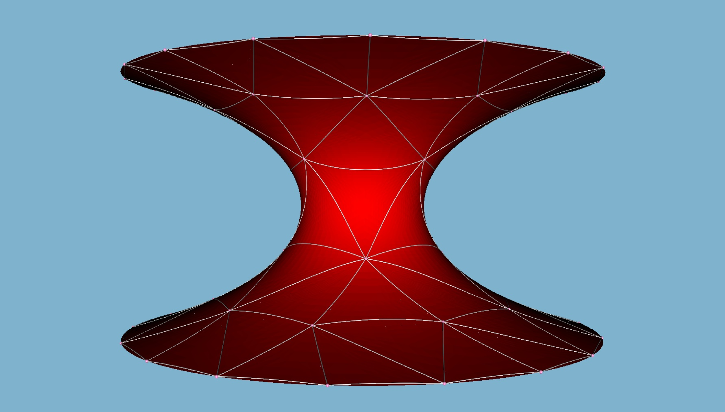
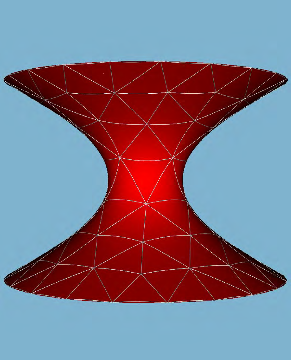
Figure 9: Nodoids generated by the revolution of C 1 subscript 𝐶 1 C_{1} C 2 subscript 𝐶 2 C_{2}
E = a 2 b 2 ( c cosh ( t ) + a ) 2 , G = b 2 ( c cosh ( t ) − a ) c cosh ( t ) + a , L = − a b 2 c cosh ( t ) ( c 2 cosh 2 ( t ) − a 2 ) ( c cosh ( t ) + a ) , N = b 2 c cosh ( t ) + a , k 1 = − c cosh ( t ) a ( c cosh ( t ) − a ) , k 2 = 1 c cosh ( t ) − a , H = − 1 2 a , K = − c cosh ( t ) a ( c cosh ( t ) − a ) 2 . 𝐸 absent superscript 𝑎 2 superscript 𝑏 2 superscript 𝑐 𝑡 𝑎 2 𝐺 absent superscript 𝑏 2 𝑐 𝑡 𝑎 𝑐 𝑡 𝑎 𝐿 absent 𝑎 superscript 𝑏 2 𝑐 𝑡 superscript 𝑐 2 superscript 2 𝑡 superscript 𝑎 2 𝑐 𝑡 𝑎 𝑁 absent superscript 𝑏 2 𝑐 𝑡 𝑎 subscript 𝑘 1 absent 𝑐 𝑡 𝑎 𝑐 𝑡 𝑎 subscript 𝑘 2 absent 1 𝑐 𝑡 𝑎 𝐻 absent 1 2 𝑎 𝐾 absent 𝑐 𝑡 𝑎 superscript 𝑐 𝑡 𝑎 2 \begin{array}[]{rlrl }E=&\displaystyle\frac{a^{2}b^{2}}{\left(c\cosh(t)+a\right)^{2}},&\hskip 28.45274ptG=&\displaystyle\frac{b^{2}\left(c\cosh(t)-a\right)}{c\cosh(t)+a},\\[12.91663pt]
L=&\displaystyle\frac{-ab^{2}c\cosh(t)}{\left(c^{2}\cosh^{2}(t)-a^{2}\right)\left(c\cosh(t)+a\right)},&N=&\displaystyle\frac{b^{2}}{c\cosh(t)+a},\\[12.91663pt]
k_{1}=&\displaystyle\frac{-c\cosh(t)}{\displaystyle a(c\cosh(t)-a)},&k_{2}=&\displaystyle\frac{1}{\displaystyle c\cosh(t)-a},\\[12.91663pt]
H=&\displaystyle\frac{-1}{2a},&K=&\displaystyle\frac{-c\cosh(t)}{\displaystyle a\left(c\cosh(t)-a\right)^{2}}.\end{array}
The geodesic curvature of a parallel is
k g = c sinh ( t ) b ( c cosh ( t ) − a ) , subscript 𝑘 𝑔 𝑐 𝑡 𝑏 𝑐 𝑡 𝑎 k_{g}=\frac{c\sinh(t)}{b\big{(}c\cosh(t)-a\big{)}},
and the total curvature is
∫ z z z z z z z z z z z z z z 1 K 𝑑 σ = − c ( v 2 − v 1 ) sinh ( t ) c 2 cosh 2 ( t ) − a 2 | t 1 t 2 . subscript subscript z z z z z z z z z z z z z z 1 𝐾 differential-d 𝜎 evaluated-at 𝑐 subscript 𝑣 2 subscript 𝑣 1 𝑡 superscript 𝑐 2 superscript 2 𝑡 superscript 𝑎 2 subscript 𝑡 1 subscript 𝑡 2 \int_{\kern-0.23103pt\hbox{$z$}\kern-3.5632pt\kern 0.07701pt\hbox{$z$}\kern-3.5632pt\kern 0.07701pt\hbox{$z$}\kern-3.5632pt\kern 0.07701pt\hbox{$z$}\kern-3.5632pt\kern 0.07701pt\hbox{$z$}\kern-3.5632pt\kern 0.07701pt\hbox{$z$}\kern-3.5632pt\kern 0.07701pt\hbox{$z$}\kern-3.5632pt\kern-0.38495pt\raise 0.105pt\hbox{$z$}\kern-3.5632pt\kern 0.07701pt\raise 0.105pt\hbox{$z$}\kern-3.5632pt\kern 0.07701pt\raise 0.105pt\hbox{$z$}\kern-3.5632pt\kern 0.07701pt\raise-0.105pt\hbox{$z$}\kern-3.5632pt\kern 0.07701pt\raise-0.105pt\hbox{$z$}\kern-3.5632pt\kern-0.15402pt\hbox{$z$}\kern-3.5632pt\raise-0.105pt\hbox{$z$}_{1}}Kd\sigma=-c(v_{2}-v_{1})\left.\frac{\sinh(t)}{\sqrt{c^{2}\cosh^{2}(t)-a^{2}}}\right|_{t_{1}}^{t_{2}}.
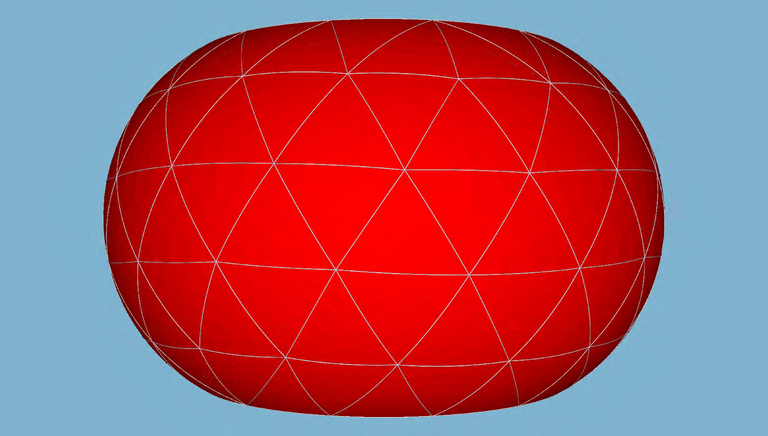
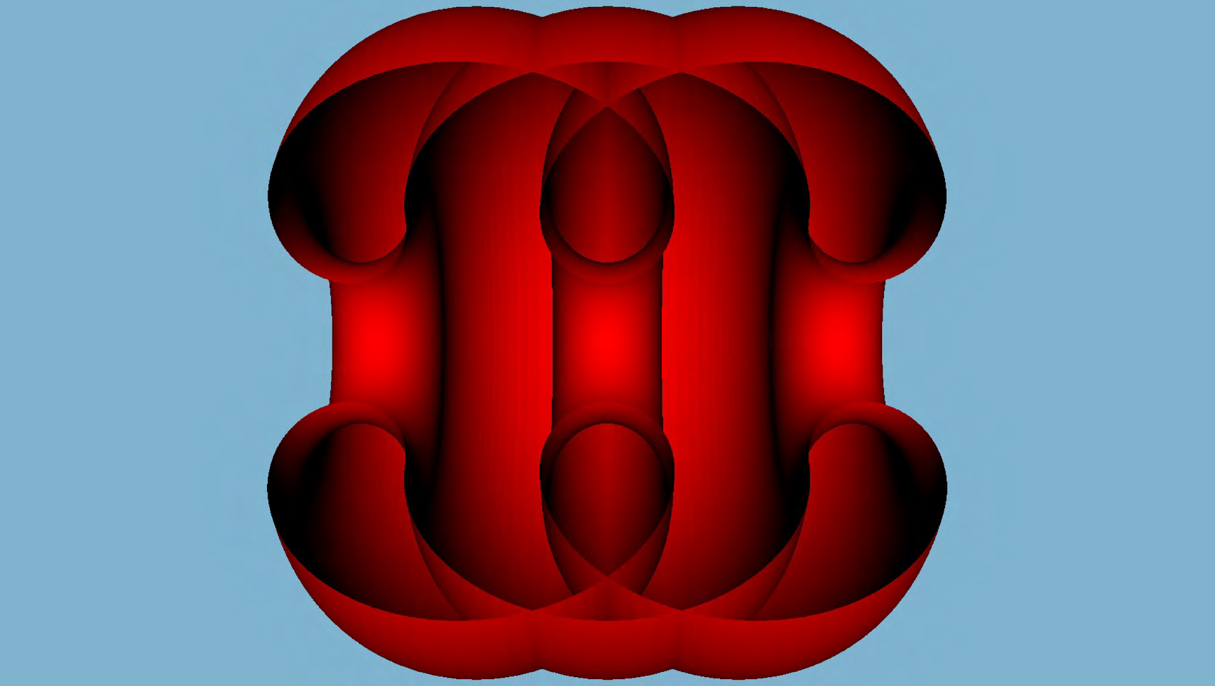
Figure 10: Left: Closed nodoid (compact without boundary), connected sum of 4 tori.
Right: Connected compact nodoid with boundary.
Nodoid2: z z z z z z z z z z z z z z 2 ( t , v ) = ( f 2 ( t ) cos ( v ) , f 2 ( t ) sin ( v ) , g 2 ( t ) ) , subscript z z z z z z z z z z z z z z 2 𝑡 𝑣 subscript 𝑓 2 𝑡 𝑣 subscript 𝑓 2 𝑡 𝑣 subscript 𝑔 2 𝑡 \kern-0.33005pt\hbox{$z$}\kern-5.0903pt\kern 0.11002pt\hbox{$z$}\kern-5.0903pt\kern 0.11002pt\hbox{$z$}\kern-5.0903pt\kern 0.11002pt\hbox{$z$}\kern-5.0903pt\kern 0.11002pt\hbox{$z$}\kern-5.0903pt\kern 0.11002pt\hbox{$z$}\kern-5.0903pt\kern 0.11002pt\hbox{$z$}\kern-5.0903pt\kern-0.54993pt\raise 0.15pt\hbox{$z$}\kern-5.0903pt\kern 0.11002pt\raise 0.15pt\hbox{$z$}\kern-5.0903pt\kern 0.11002pt\raise 0.15pt\hbox{$z$}\kern-5.0903pt\kern 0.11002pt\raise-0.15pt\hbox{$z$}\kern-5.0903pt\kern 0.11002pt\raise-0.15pt\hbox{$z$}\kern-5.0903pt\kern-0.22003pt\hbox{$z$}\kern-5.0903pt\raise-0.15pt\hbox{$z$}_{2}(t,v)=\Big{(}f_{2}(t)\cos(v),f_{2}(t)\sin(v),g_{2}(t)\Big{)}, 9
h 2 ( t ) = − a b c 2 cosh 2 ( t ) − a 2 ( c cosh ( t ) − a ) subscript ℎ 2 𝑡 𝑎 𝑏 superscript 𝑐 2 superscript 2 𝑡 superscript 𝑎 2 𝑐 𝑡 𝑎 h_{2}(t)=\frac{-ab}{\sqrt{c^{2}\cosh^{2}(t)-a^{2}}\left(c\cosh(t)-a\right)}
from which it follows that
( z z z z z z z z z z z z z z 2 ) t = ( c sinh ( t ) h 2 ( t ) cos ( v ) , c sinh ( t ) h 2 ( t ) sin ( v ) , b h 2 ( t ) ) , ( z z z z z z z z z z z z z z 2 ) v = ( − f 2 ( t ) sin ( v ) , f 2 ( t ) cos ( v ) , 0 ) . subscript subscript z z z z z z z z z z z z z z 2 𝑡 absent 𝑐 𝑡 subscript ℎ 2 𝑡 𝑣 𝑐 𝑡 subscript ℎ 2 𝑡 𝑣 𝑏 subscript ℎ 2 𝑡 subscript subscript z z z z z z z z z z z z z z 2 𝑣 absent subscript 𝑓 2 𝑡 𝑣 subscript 𝑓 2 𝑡 𝑣 0 \begin{array}[]{rl}({\kern-0.33005pt\hbox{$z$}\kern-5.0903pt\kern 0.11002pt\hbox{$z$}\kern-5.0903pt\kern 0.11002pt\hbox{$z$}\kern-5.0903pt\kern 0.11002pt\hbox{$z$}\kern-5.0903pt\kern 0.11002pt\hbox{$z$}\kern-5.0903pt\kern 0.11002pt\hbox{$z$}\kern-5.0903pt\kern 0.11002pt\hbox{$z$}\kern-5.0903pt\kern-0.54993pt\raise 0.15pt\hbox{$z$}\kern-5.0903pt\kern 0.11002pt\raise 0.15pt\hbox{$z$}\kern-5.0903pt\kern 0.11002pt\raise 0.15pt\hbox{$z$}\kern-5.0903pt\kern 0.11002pt\raise-0.15pt\hbox{$z$}\kern-5.0903pt\kern 0.11002pt\raise-0.15pt\hbox{$z$}\kern-5.0903pt\kern-0.22003pt\hbox{$z$}\kern-5.0903pt\raise-0.15pt\hbox{$z$}}_{2})_{t}=&\Big{(}c\sinh(t)h_{2}(t)\cos(v),c\sinh(t)h_{2}(t)\sin(v),bh_{2}(t)\Big{)},\\[4.30554pt]
({\kern-0.33005pt\hbox{$z$}\kern-5.0903pt\kern 0.11002pt\hbox{$z$}\kern-5.0903pt\kern 0.11002pt\hbox{$z$}\kern-5.0903pt\kern 0.11002pt\hbox{$z$}\kern-5.0903pt\kern 0.11002pt\hbox{$z$}\kern-5.0903pt\kern 0.11002pt\hbox{$z$}\kern-5.0903pt\kern 0.11002pt\hbox{$z$}\kern-5.0903pt\kern-0.54993pt\raise 0.15pt\hbox{$z$}\kern-5.0903pt\kern 0.11002pt\raise 0.15pt\hbox{$z$}\kern-5.0903pt\kern 0.11002pt\raise 0.15pt\hbox{$z$}\kern-5.0903pt\kern 0.11002pt\raise-0.15pt\hbox{$z$}\kern-5.0903pt\kern 0.11002pt\raise-0.15pt\hbox{$z$}\kern-5.0903pt\kern-0.22003pt\hbox{$z$}\kern-5.0903pt\raise-0.15pt\hbox{$z$}}_{2})_{v}=&\Big{(}-f_{2}(t)\sin(v),f_{2}(t)\cos(v),0\Big{)}.\end{array}
The unit normal vector at ( t , v ) 𝑡 𝑣 (t,v)
n n n n n n n n n n n n n n 2 ( t , v ) = ( b cos ( v ) c 2 cosh 2 ( t ) − a 2 , b sin ( v ) c 2 cosh 2 ( t ) − a 2 , − c sinh ( t ) c 2 cosh 2 ( t ) − a 2 ) . subscript n n n n n n n n n n n n n n 2 𝑡 𝑣 𝑏 𝑣 superscript 𝑐 2 superscript 2 𝑡 superscript 𝑎 2 𝑏 𝑣 superscript 𝑐 2 superscript 2 𝑡 superscript 𝑎 2 𝑐 𝑡 superscript 𝑐 2 superscript 2 𝑡 superscript 𝑎 2 {\kern-0.33005pt\hbox{$n$}\kern-6.00235pt\kern 0.11002pt\hbox{$n$}\kern-6.00235pt\kern 0.11002pt\hbox{$n$}\kern-6.00235pt\kern 0.11002pt\hbox{$n$}\kern-6.00235pt\kern 0.11002pt\hbox{$n$}\kern-6.00235pt\kern 0.11002pt\hbox{$n$}\kern-6.00235pt\kern 0.11002pt\hbox{$n$}\kern-6.00235pt\kern-0.54993pt\raise 0.15pt\hbox{$n$}\kern-6.00235pt\kern 0.11002pt\raise 0.15pt\hbox{$n$}\kern-6.00235pt\kern 0.11002pt\raise 0.15pt\hbox{$n$}\kern-6.00235pt\kern 0.11002pt\raise-0.15pt\hbox{$n$}\kern-6.00235pt\kern 0.11002pt\raise-0.15pt\hbox{$n$}\kern-6.00235pt\kern-0.22003pt\hbox{$n$}\kern-6.00235pt\raise-0.15pt\hbox{$n$}}_{2}(t,v)=\left(\frac{b\cos(v)}{\sqrt{c^{2}\cosh^{2}(t)-a^{2}}},\frac{b\sin(v)}{\sqrt{c^{2}\cosh^{2}(t)-a^{2}}},-\frac{c\sinh(t)}{\sqrt{c^{2}\cosh^{2}(t)-a^{2}}}\right).
E = a 2 b 2 ( c cosh ( t ) − a ) 2 , G = b 2 ( c cosh ( t ) + a ) c cosh ( t ) − a , L = − a b 2 c cosh ( t ) ( c 2 cosh 2 ( t ) − a 2 ) ( c cosh ( t ) − a ) , N = − b 2 c cosh ( t ) − a , k 1 = − c cosh ( t ) a ( c cosh ( t ) + a ) , k 2 = − 1 c cosh ( t ) + a , H = − 1 2 a , K = c cosh ( t ) a ( c cosh ( t ) + a ) 2 . 𝐸 absent superscript 𝑎 2 superscript 𝑏 2 superscript 𝑐 𝑡 𝑎 2 𝐺 absent superscript 𝑏 2 𝑐 𝑡 𝑎 𝑐 𝑡 𝑎 𝐿 absent 𝑎 superscript 𝑏 2 𝑐 𝑡 superscript 𝑐 2 superscript 2 𝑡 superscript 𝑎 2 𝑐 𝑡 𝑎 𝑁 absent superscript 𝑏 2 𝑐 𝑡 𝑎 subscript 𝑘 1 absent 𝑐 𝑡 𝑎 𝑐 𝑡 𝑎 subscript 𝑘 2 absent 1 𝑐 𝑡 𝑎 𝐻 absent 1 2 𝑎 𝐾 absent 𝑐 𝑡 𝑎 superscript 𝑐 𝑡 𝑎 2 \begin{array}[]{rlrl }E=&\displaystyle\frac{a^{2}b^{2}}{\left(c\cosh(t)-a\right)^{2}},&\hskip 28.45274ptG=&\displaystyle\frac{b^{2}\left(c\cosh(t)+a\right)}{c\cosh(t)-a},\\[12.91663pt]
L=&\displaystyle\frac{-ab^{2}c\cosh(t)}{\left(c^{2}\cosh^{2}(t)-a^{2}\right)\left(c\cosh(t)-a\right)},&N=&\displaystyle\displaystyle\frac{-b^{2}}{c\cosh(t)-a},\\[12.91663pt]
k_{1}=&\displaystyle\frac{-c\cosh(t)}{\displaystyle a(c\cosh(t)+a)},&k_{2}=&\displaystyle\frac{-1}{\displaystyle c\cosh(t)+a},\\[12.91663pt]
H=&\displaystyle\frac{-1}{2a},&K=&\displaystyle\frac{c\cosh(t)}{\displaystyle a\left(c\cosh(t)+a\right)^{2}}.\end{array}
The geodesic curvature of a parallel is
k g = − c sinh ( t ) b ( c cosh ( t ) + a ) . subscript 𝑘 𝑔 𝑐 𝑡 𝑏 𝑐 𝑡 𝑎 k_{g}=\frac{-c\sinh(t)}{b\big{(}c\cosh(t)+a\big{)}}.
The total curvature is
∫ z z z z z z z z z z z z z z 2 K 𝑑 σ = c ( v 2 − v 1 ) sinh ( t ) c 2 cosh 2 ( t ) − a 2 | t 1 t 2 . subscript subscript z z z z z z z z z z z z z z 2 𝐾 differential-d 𝜎 evaluated-at 𝑐 subscript 𝑣 2 subscript 𝑣 1 𝑡 superscript 𝑐 2 superscript 2 𝑡 superscript 𝑎 2 subscript 𝑡 1 subscript 𝑡 2 \int_{\kern-0.23103pt\hbox{$z$}\kern-3.5632pt\kern 0.07701pt\hbox{$z$}\kern-3.5632pt\kern 0.07701pt\hbox{$z$}\kern-3.5632pt\kern 0.07701pt\hbox{$z$}\kern-3.5632pt\kern 0.07701pt\hbox{$z$}\kern-3.5632pt\kern 0.07701pt\hbox{$z$}\kern-3.5632pt\kern 0.07701pt\hbox{$z$}\kern-3.5632pt\kern-0.38495pt\raise 0.105pt\hbox{$z$}\kern-3.5632pt\kern 0.07701pt\raise 0.105pt\hbox{$z$}\kern-3.5632pt\kern 0.07701pt\raise 0.105pt\hbox{$z$}\kern-3.5632pt\kern 0.07701pt\raise-0.105pt\hbox{$z$}\kern-3.5632pt\kern 0.07701pt\raise-0.105pt\hbox{$z$}\kern-3.5632pt\kern-0.15402pt\hbox{$z$}\kern-3.5632pt\raise-0.105pt\hbox{$z$}_{2}}Kd\sigma=c(v_{2}-v_{1})\left.\frac{\sinh(t)}{\sqrt{c^{2}\cosh^{2}(t)-a^{2}}}\right|_{t_{1}}^{t_{2}}.
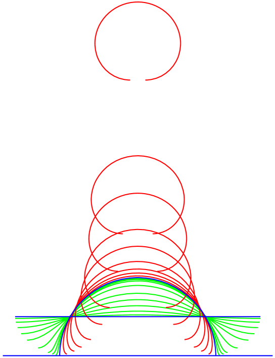
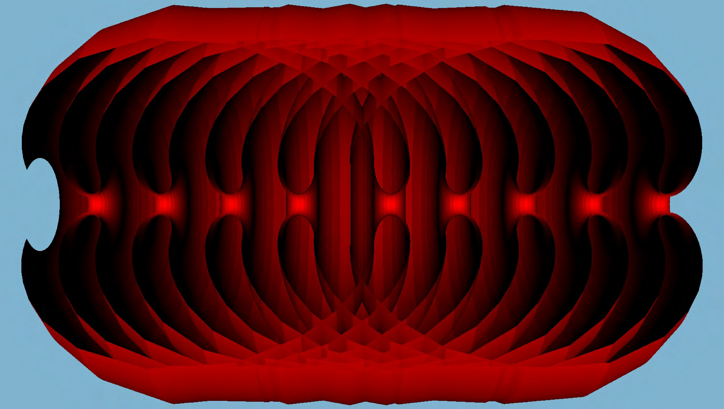
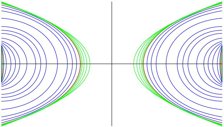
Figure 11: Planar sections containing the revolution axis of a family of Delaunay surfaces with constant volume.
From the outside-in: cylinder (black), unduloids (green), catenoid (red), nodoids (blue), catenoid (red) and unduloids (green).
Fig. 10 C ∞ superscript 𝐶 C^{\infty}
Delaunay surfaces are characterized by minimizing the area with fixed boundaries and constant volume. Here we illustrate the
versatility of our formulation by finding a surface which satisfies these conditions. Consider a plane curve ( f ( t ) , g ( t ) ) 𝑓 𝑡 𝑔 𝑡 (f(t),g(t)) π ∫ t 0 t 1 f 2 ( t ) g ′ ( t ) 𝑑 t 𝜋 superscript subscript subscript 𝑡 0 subscript 𝑡 1 superscript 𝑓 2 𝑡 superscript 𝑔 ′ 𝑡 differential-d 𝑡 \pi\int_{t_{0}}^{t_{1}}f^{2}(t)g^{\prime}(t)dt ( f ( t 0 ) , g ( t 0 ) ) = ( f 0 , g 0 ) 𝑓 subscript 𝑡 0 𝑔 subscript 𝑡 0 subscript 𝑓 0 subscript 𝑔 0 \left(f(t_{0}),g(t_{0})\right)=(f_{0},g_{0}) ( f ( t 1 ) , g ( t 1 ) ) = ( f 1 , g 1 ) 𝑓 subscript 𝑡 1 𝑔 subscript 𝑡 1 subscript 𝑓 1 subscript 𝑔 1 \left(f(t_{1}),g(t_{1})\right)=(f_{1},g_{1})
Consider for example the symmetric nodoid generated by a roulette C 1 subscript 𝐶 1 C_{1} ± t 0 plus-or-minus subscript 𝑡 0 \pm t_{0} a 𝑎 a b 𝑏 b
π a b 4 ∫ − t 0 t 0 ( c cosh ( t ) − a ) ( c cosh ( t ) + a ) 2 c 2 cosh 2 ( t ) − a 2 𝑑 t = 1 , b ( c cosh ( t 0 ) − a ) c 2 cosh 2 ( t 0 ) − a 2 = 1 . 𝜋 𝑎 superscript 𝑏 4 superscript subscript subscript 𝑡 0 subscript 𝑡 0 𝑐 𝑡 𝑎 superscript 𝑐 𝑡 𝑎 2 superscript 𝑐 2 superscript 2 𝑡 superscript 𝑎 2 differential-d 𝑡 absent 1 missing-subexpression missing-subexpression 𝑏 𝑐 subscript 𝑡 0 𝑎 superscript 𝑐 2 superscript 2 subscript 𝑡 0 superscript 𝑎 2 absent 1 missing-subexpression missing-subexpression \begin{array}[]{rlrl }\displaystyle\pi ab^{4}\int_{-t_{0}}^{t_{0}}\frac{\left(c\cosh(t)-a\right)}{\left(c\cosh(t)+a\right)^{2}\sqrt{c^{2}\cosh^{2}(t)-a^{2}}}dt&=1,\\[21.52771pt]
\displaystyle\frac{b\left(c\cosh(t_{0})-a\right)}{\sqrt{c^{2}\cosh^{2}(t_{0})-a^{2}}}&=1.\end{array}
In Fig 11 t 0 subscript 𝑡 0 t_{0}
Finally the paremetrizations developed here have proven extremely useful in analytic and computational
explorations of the structure of crystalline particle arrays on Delaunay surfaces as realized experimentally
in capillary bridges [10 ] .
Acknowledgments. This work has been partly supported by the Spanish Research Council (Comisión
Interministerial de Ciencia y Tecnología,) under project MTM2010-19660. The work of M.J.B. was also supported by the
National Science Foundation through Grant No. DMR-1004789 and by funds from the Soft Matter Program of Syracuse University.