Determination of $\tan\beta$ from the Higgs boson decay at linear colliders

Abstract

In the two Higgs doublet model, $\tan\beta$ is an important parameter, which is defined as the ratio of the vacuum expectation values of the doublets. We study how accurately $\tan\beta$ can be determined at linear colliders via the precision measurement of the decay branching fraction of the standard model (SM) like Higgs boson. Since the effective coupling constants of the Higgs boson with the weak gauge bosons are expected to be measured accurately, the branching ratios can be precisely determined. Consequently, $\tan\beta$ can be determined with a certain amount of accuracy. Comparing the method to those using direct production of the additional Higgs bosons, we find that, depending on the type of Yukawa interactions, the precision measurement of the decay of the SM-like Higgs boson can be the best way to determine $\tan\beta$, when the deviations in the coupling constants with the gauge boson from the SM prediction are observed at linear colliders.

I Introduction

A Higgs boson has been discovered at the LHC Ref:atlas ; Ref:cms . Current data show that its properties such as its mass, production cross sections times the decay branching ratios and the spin-parity are consistent with those of the Higgs boson in the standard model (SM) Ref:atlas-comb ; Ref:cms-comb . However, the whole structure of the Higgs sector has not been clarified at all. Since there is no principle to determine the structure of the Higgs sector, the SM Higgs sector is the simplest but just one of the possibilities. There are many problems, which should be explained by new physics beyond the SM, such as the naturalness problem, the origin of tiny neutrino masses and mixings, the existence of dark matter, etc. Various extensions of the SM considered to solve these problems often contain the extended Higgs sector, where new Higgs multiplets are added to the SM Higgs sector.

Multi Higgs models are constrained by the electroweak $\rho$ parameter significantly. The two Higgs doublet model (THDM) is the natural and minimal extension of the SM Higgs sector, since multi Higgs doublet models predict the $\rho$ parameter to be unity at the tree level Ref:HHG . In general, the THDM predicts the flavor changing neutral current (FCNC) which is severely constrained by the experimental data. This problem may be solved by introducing a discrete $Z_{2}$ symmetry under which the different parity is assigned to each doublet field Ref:GW . Under this symmetry, each fermion couples with only one Higgs doublet, and hence the FCNC is absent at the tree level. Depending on the assignment of the $Z_{2}$ parity to each fermion, there are four types of Yukawa interactions in the THDM. Among the four types of Yukawa interactions, so-called Type-II and Type-X Ref:2hdm deserve many interests as an effective theory of the Higgs sector in the new physics model. For example, the Type-II THDM is known to be the Higgs sector in the minimal supersymmetric extension of the SM (MSSM) Ref:HK ; Ref:Djouadi2 , where one Higgs doublet couples with down-type quarks and charged leptons and the other with up-type quarks. On the other hand, the Type-X THDM, in which one Higgs doublet couples with quarks and the other with charged leptons, may be motivated by some sort of new physics models concerning phenomena relevant to leptons and Higgs bosons, such as tiny neutrino masses Ref:U1X ; Ref:AKS , the positron cosmic ray anomaly Ref:GHK , the Fermi-LAT gamma ray line data Ref:BBES , the muon anomalous magnetic moment Ref:CWWY , etc.

Verification of the THDM by using the collider data and the flavor data has been an important task, while no positive evidence has been found so far. The results give constraints on the parameters in the THDM, depending on the type of the Yukawa interactions Ref:mssm-HA-atlas ; Ref:mssm-HA-cms ; Ref:2HDM-LHC ; Ref:bsg ; Ref:bsg2 ; Ref:btaunu ; Ref:tau . Some of them are not constrained so strongly because of the small couplings of additional Higgs bosons with quarks, allowing a relatively light mass of extra Higgs bosons Ref:TypeX ; Ref:AKTY ; Ref:Su ; Ref:Logan . Further studies will be continued at the upgraded LHC with $\sqrt{s}=14$ TeV, where the discovery of more heavier particles may be expected.

On the other hand, evidences of the THDM can be probed through the measurement of the SM-like Higgs boson, since the coupling constants of the SM-like Higgs boson can deviate from those in the SM. This is quite a realistic situation, since the Higgs couplings can be measured very precisely, a few percent level, at the International Linear Collider (ILC) Ref:h-BR ; Ref:ilc-TDR ; Ref:ilc-Peskin . It may be problematic that it is not straightforward to identify the model of new physics from such measurements, since the effects are indirect and some models may bring the similar effects. To resolve this problem, one needs to combine measurements of various observables and perform fingerprinting of the models which predict different patterns of the deviations in the various observables.

In this paper, we focus on the determination of $\tan\beta$, the ratio of vacuum expectation values of the doublets in the THDMs, by using future precision measurements of the SM-like Higgs boson at linear colliders. So far, the methods to determine $\tan\beta$ have been discussed using the heavy extra Higgs bosons within the context of the MSSM Ref:TanB . However, the methods using the heavy extra bosons must follow the discovery of them. Thus, these are applicable to the cases with relatively small masses, where already strong constraints are obtained in some types of the THDM Ref:mssm-HA-atlas ; Ref:mssm-HA-cms ; Ref:mssm-H+ . On the other hand, we propose a new method to determine $\tan\beta$, through the branching ratios of the SM-like Higgs boson, which could be performed even when the discovery of extra Higgs bosons is not accomplished. Our method is applicable when there exists a deviation in the gauge couplings of the SM-like Higgs boson. In the general THDM, the deviation can be larger than that in the MSSM, since $\tan\beta$ is independent of the masses of the extra Higgs bosons. Thus, it is meaningful to investigate the $\tan\beta$ measurement in various situations in the masses of extra Higgs bosons. We evaluate the uncertainties of the $\tan\beta$ determination in our method in the general THDM, and compare them with those of the methods proposed previously.

This paper is organized as follows. In Section II, we give a brief review on the THDM to specify the notation and define the parameters relevant in our study. In Section III, three methods for the $\tan\beta$ determination are introduced; i) the branching ratio measurement, ii) the total width measurement of the extra Higgs bosons, and iii) the precision measurement of the decay branching ratios of the SM-like Higgs boson. We apply these methods to the Type-II and Type-X THDMs. The simulation details are summarized in Appendix A. Conclusion and discussion are given in Section IV.

II The Two Higgs Doublet Model

In the THDM, the SU(2) doublet scalar fields with a hypercharge $Y=1/2$ are parametrized as

$$\Phi_{i}=\begin{pmatrix}i\,\omega_{i}^{+}\\ \frac{1}{\sqrt{2}}(v_{i}+h_{i}-i\,z_{i})\end{pmatrix},$$ (1)

where $i=1,2$. The mass eigenstates are defined by introducing the mixing angles, $\alpha$ and $\beta$, as

$$\begin{pmatrix}h_{1}\\ h_{2}\end{pmatrix}=\begin{pmatrix}\cos\alpha&-\sin\alpha\\ \sin\alpha&\cos\alpha\end{pmatrix}\begin{pmatrix}H\\ h\end{pmatrix},\,\begin{pmatrix}z_{1}\\ z_{2}\end{pmatrix}=\begin{pmatrix}\cos\beta&-\sin\beta\\ \sin\beta&\cos\beta\end{pmatrix}\begin{pmatrix}z\\ A\end{pmatrix},\,\begin{pmatrix}\omega_{1}^{+}\\ \omega_{2}^{+}\end{pmatrix}=\begin{pmatrix}\cos\beta&-\sin\beta\\ \sin\beta&\cos\beta\end{pmatrix}\begin{pmatrix}\omega^{+}\\ H^{+}\end{pmatrix},$$ (2)

where $\beta$ satisfies $\tan\beta=v_{2}/v_{1}$. For simplicity, we assume CP conservation in the Higgs sector. Then, there are five physical Higgs bosons, which are two CP-even states $(h,H)$, one CP-odd state $A$, and a pair of the charged states $H^{\pm}$. The electroweak Nambu-Goldstone bosons, $z,\omega^{\pm}$, are absorbed into the weak gauge bosons. For the details of the Higgs potential in the THDM, see, e.g., Ref. Ref:KOSY .

Gauge interactions of Higgs bosons in the THDM are given by normalizing them with those in the SM as

$$\frac{g^{\rm THDM}_{hVV}}{g^{\rm SM}_{hVV}}=\sin(\beta-\alpha),\quad\frac{g^{\rm THDM}_{HVV}}{g^{\rm SM}_{hVV}}=\cos(\beta-\alpha),$$ (3)

for $V=Z,W$. Thus, when $\sin(\beta-\alpha)=1$, which is so-called “the SM-like limit”, $h$ has the same gauge interaction as the SM Higgs boson. We note that the deviation from the SM-like limit is theoretically restricted for heavy $H$ and $A$ in the general THDM Ref:Uni-2hdm . Indeed, for $m_{h}^{2}\ll m_{H}^{2},M^{2}$ with large $\tan\beta$, $\sin(\beta-\alpha)$ can be written as $\sin^{2}(\beta-\alpha)\simeq 1+\lambda_{1}v^{2}/(m_{H}^{2}\tan^{2}\beta)$ with $\lambda_{1}$ being a coefficient of the quartic term in the potential. A large value of $\lambda_{1}$ is constrained by requiring the validity of the perturbative calculation (so-called unitarity bound) Ref:Uni-2hdm . Thus, the deviation from the SM-like limit cannot be large for heavy $H$ and $A$.

Under the $Z_{2}$ symmetry, there are four types of the $Z_{2}$ parity assignment to the SM fermions, as listed in TABLE 1.

	$\Phi_{1}$	$\Phi_{2}$	$u_{R}$	$d_{R}$	$\ell_{R}$	$Q_{L}$, $L_{L}$
Type-I	$+$	$-$	$-$	$-$	$-$	$+$
Type-II	$+$	$-$	$-$	$+$	$+$	$+$
Type-X	$+$	$-$	$-$	$-$	$+$	$+$
Type-Y	$+$	$-$	$-$	$+$	$-$	$+$

Table 1: Parity assignments under the softly broken $Z_{2}$ symmetry Ref:AKTY .

Then, Yukawa interactions of the SM fermions to the Higgs bosons are given by

$${\mathcal{L}}_{\text{Yukawa}}^{\text{THDM}}= -{\overline{Q}}_{L}Y_{u}\widetilde{\Phi}_{u}u_{R}-{\overline{Q}}_{L}Y_{d}\Phi_{d}d_{R}-{\overline{L}}_{L}Y_{\ell}\Phi_{\ell}\ell_{R}+\text{H.c.},$$ (4)

where $\Phi_{f}$ ($f=u,d$ or $\ell$) is selected from $\Phi_{1}$ or $\Phi_{2}$ to make each vertex $Z_{2}$-invariant. In terms of the mass eigenstates, the Yukawa interactions are expressed as

$${\mathcal{L}}_{\text{Yukawa}}^{\text{THDM}}= -\sum_{f=u,d,\ell}\Bigl{[}+\frac{m_{f}}{v}\,\xi_{h}^{f}\,{\overline{f}}fh+\frac{m_{f}}{v}\,\xi_{H}^{f}\,{\overline{f}}fH-i\frac{m_{f}}{v}\,\xi_{A}^{f}\,{\overline{f}}\gamma_{5}fA\Bigr{]}$$

$$-\Bigl{\{}+\frac{\sqrt{2}V_{ud}}{v}\,\overline{u}\bigl{[}+m_{u}\,\xi_{A}^{u}\,\text{P}_{L}+m_{d}\,\xi_{A}^{d}\,\text{P}_{R}\bigr{]}d\,H^{+}+\frac{\sqrt{2}\,m_{\ell}}{v}\xi_{A}^{\ell}\,\overline{\nu_{L}}\ell_{R}H^{+}+\text{H.c.}\Bigr{\}},$$ (5)

where $P_{L(R)}$ are projection operators for left-(right-)handed fermions. The scaling factors $\xi_{\phi}^{f}$ ($\phi=h,H,A$) are listed in TABLE 2.

	$\xi_{h}^{u}$	$\xi_{h}^{d}$	$\xi_{h}^{\ell}$	$\xi_{H}^{u}$	$\xi_{H}^{d}$	$\xi_{H}^{\ell}$	$\xi_{A}^{u}$	$\xi_{A}^{d}$	$\xi_{A}^{\ell}$
Type-I	$c_{\alpha}/s_{\beta}$	$c_{\alpha}/s_{\beta}$	$c_{\alpha}/s_{\beta}$	$s_{\alpha}/s_{\beta}$	$s_{\alpha}/s_{\beta}$	$s_{\alpha}/s_{\beta}$	$\cot\beta$	$-\cot\beta$	$-\cot\beta$
Type-II	$c_{\alpha}/s_{\beta}$	$-s_{\alpha}/c_{\beta}$	$-s_{\alpha}/c_{\beta}$	$s_{\alpha}/s_{\beta}$	$c_{\alpha}/c_{\beta}$	$c_{\alpha}/c_{\beta}$	$\cot\beta$	$\tan\beta$	$\tan\beta$
Type-X	$c_{\alpha}/s_{\beta}$	$c_{\alpha}/s_{\beta}$	$-s_{\alpha}/c_{\beta}$	$s_{\alpha}/s_{\beta}$	$s_{\alpha}/s_{\beta}$	$c_{\alpha}/c_{\beta}$	$\cot\beta$	$-\cot\beta$	$\tan\beta$
Type-Y	$c_{\alpha}/s_{\beta}$	$-s_{\alpha}/c_{\beta}$	$c_{\alpha}/s_{\beta}$	$s_{\alpha}/s_{\beta}$	$c_{\alpha}/c_{\beta}$	$s_{\alpha}/s_{\beta}$	$\cot\beta$	$\tan\beta$	$-\cot\beta$

Table 2: The scaling factors in each type of Yukawa interactions in Eq. (5) Ref:AKTY .

Corrections to the Yukawa coupling constants of $h$ are $\xi^{f}_{h}=\sin(\beta-\alpha)+\cot\beta\cdot\cos(\beta-\alpha)$ for $f$=$u$ in Type-II and $f$=$u,d$ in Type-X, and $\xi^{f}_{h}=\sin(\beta-\alpha)-\tan\beta\cdot\cos(\beta-\alpha)$ for $f$=$d,\ell$ in Type-II and $f$=$\ell$ in Type-X. Thus, in the SM-like limit, the $\tan\beta$ dependence disappears in $\xi^{f}_{h}$, and the Yukawa interactions of $h$ reduce to those in the SM as well. Otherwise, there is a $\tan\beta$ dependence in $\xi^{f}_{h}$. For the Yukawa coupling constants of $H$ and $A$, these depend significantly on $\tan\beta$ around the SM-like limit.

The $\tan\beta$ dependence in the Yukawa coupling constants can be seen in the branching ratios of the Higgs bosons Ref:AKTY . In the Type-II and Type-X THDMs with large $\tan\beta$, a decay of $H$ and $A$ into $b\bar{b}$ and $\tau\tau$ is expected to be dominant, respectively. In FIG. 1, we evaluate the $\tan\beta$ dependence in the branching ratios of $H,A$ and also $h$ into $b\bar{b}$ in the Type-II THDM. The three panels correspond to the cases with $\sin^{2}(\beta-\alpha)=1$ (left), 0.99 (middle) and 0.98 (right), and the case with $\cos(\beta-\alpha)\leq 0$ ($\cos(\beta-\alpha)\geq 0$) is plotted in the solid (dashed) curves. For each panel, ${\mathcal{B}}^{\phi}_{bb}\equiv{\mathcal{B}}(\phi\to b\bar{b})$ for $\phi=h$, $H$ and $A$ are plotted in black, red and blue curves respectively. Here, the masses of $H$ and $A$ are taken commonly to be $200$ GeV. The branching ratios ${\mathcal{B}}_{bb}$ for $H$ and $A$ grow with $\tan\beta$, and reach a saturation point above which the values are fixed to ${\mathcal{B}}_{bb}\simeq 0.9$ (and the rest is ${\mathcal{B}}_{\tau\tau}\simeq 0.1$). A slightly large $\sin(\beta-\alpha)$ dependence in ${\mathcal{B}}^{H}_{bb}$ comes from the $H\to W^{+}W^{-}$ and $ZZ$ decay modes which rapidly increases with $\cos^{2}(\beta-\alpha)$. On the other hand, for ${\mathcal{B}}^{h}_{bb}$, there is no $\tan\beta$ dependence in the SM-like limit. However, once $\sin(\beta-\alpha)$ deviates from unity, ${\mathcal{B}}^{h}_{bb}$ shows a significant $\tan\beta$ dependence, with a large difference by the sign of $\cos(\beta-\alpha)$. Thus, the deviation from the SM-like limit, $\sin(\beta-\alpha)-1$, triggers the $\tan\beta$ dependence in ${\mathcal{B}}^{h}_{bb}$. We note that $\sin^{2}(\beta-\alpha)$ should be measured very accurately by a few percent Ref:Zh-lep , by using the cross section measurement of the $e^{+}e^{-}\to Zh$ process at the ILC. On the other hand, the determination of the sign of $\cos(\beta-\alpha)$ is not straightforward. In the following discussion, we present the analysis for fixed $\sin(\beta-\alpha)$ values in the cases of a positive and negative sign of $\cos(\beta-\alpha)$. We note that $\cos(\beta-\alpha)<0$ is derived in the MSSM.

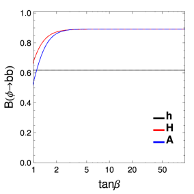
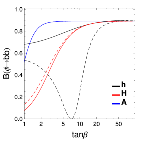
Figure 1: The decay branching ratios are shown as a function of $\tan\beta$ for a fixed $\sin^{2}(\beta-\alpha)$ for $h\to b\bar{b}$ (black curves), $H\to b\bar{b}$ (red curves), and $A\to b\bar{b}$ (blue curves) decays in the Type-II THDM. From left to right, $\sin^{2}(\beta-\alpha)$ is taken to be $1$, $0.99$, and $0.98$. The solid (dashed) curves denote the case with $\cos(\beta-\alpha)\leq 0$ ($\cos(\beta-\alpha)\geq 0$).

In FIG. 2, $\tan\beta$ dependences in the branching ratios for $h\to\tau\tau$ (black curves), $H\to\tau\tau$ (red curves) and $A\to\tau\tau$ (blue curves) decays in the Type-X THDM are plotted, where the results of $\sin^{2}(\beta-\alpha)=1$ (left panel), 0.99 (middle) and 0.98 (right) with $\cos(\beta-\alpha)\leq 0$ (solid curves) and $\cos(\beta-\alpha)\geq 0$ (dashed) are considered. The masses of $H$ and $A$ are fixed to be $200$ GeV. The qualitative features are almost similar with those in the Type-II. The branching ratios reach a saturation point close to unity at a rather large $\tan\beta$ value.

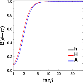
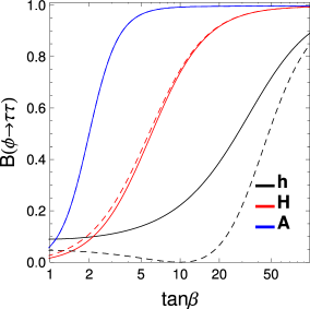
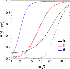
Figure 2: The decay branching ratios are shown as a function of $\tan\beta$ with a fixed value of $\sin^{2}(\beta-\alpha)$ for $h\to\tau\tau$ (black curves), for $H\to\tau\tau$ (red curves), and for $A\to\tau\tau$ (blue curves) in the Type-X THDM. From left to right, $\sin^{2}(\beta-\alpha)$ is taken to be $1$, $0.99$, and $0.98$. The solid (dashed) curves denote the case with $\cos(\beta-\alpha)\leq 0$ ($\cos(\beta-\alpha)\geq 0$).

III The $\tan\beta$ determination

In this section, we investigate the methods for the determination of $\tan\beta$ in the THDM at linear colliders. In Ref. Ref:TanB , methods by using the production and decays of $H$ and $A$ at linear colliders are studied in a context of the MSSM. In addition, we propose to utilize the precise measurement of the decay branching ratios of $h$, and compare its sensitivity with those of the previous methods in Ref. Ref:TanB . Then, we calculate the accuracy of the determination of $\tan\beta$ in the Type-II and Type-X THDMs by three methods which are described as follows:

(i) The first method is based on the measurement of the branching ratios of $H$ and $A$ in the $e^{+}e^{-}\to HA$ process Ref:TanB . Since the masses of the neutral Higgs bosons can be measured by the invariant mass distributions in an appropriate decay mode, the branching ratios can be predicted as a function of $\tan\beta$. Thus, $\tan\beta$ can be determined by measuring the decay branching ratios of $H$ and $A$. Because the $\tan\beta$ dependence in the branching ratios is large in the relatively small $\tan\beta$ regions, as we see in Figs. 1 and 2, the method is useful for those regions.

(ii) The second method is based on the measurement of the total decay widths of $H$ and $A$ Ref:TanB . For large $\tan\beta$, the total decay widths of $H$ and $A$ are governed by the $b\bar{b}~{}$ and $\tau\tau$ decay modes in the Type-II and Type-X THDMs, respectively, whose partial decay widths are proportional to $(\tan\beta)^{2}$. If the total decay widths are wider than the detector resolution for the invariant mass measurement, we can directly measure the absolute value of the total decay widths. Thus, $\tan\beta$ can be extracted from the total decay widths in the large $\tan\beta$ regions.

(iii) In addition to these two methods, we propose to utilize the precision measurement of the decay branching ratios of $h$. For $m_{h}=125$ GeV, the main decay modes of $h$ are expected to be measured precisely by a few percent level at the ILC Ref:h-BR . In the THDM, the decay branching ratios of $h$ depend on $\tan\beta$, as long as $\sin(\beta-\alpha)<1$ which can be determined independently. This means that the precision measurement of the decay of $h$ can probe $\tan\beta$.

In the following subsections, we show the detailed analysis of these methods in the Type-II and Type-X THDMs. We also comment on the cases for the other types in the THDM.

III.1 Sensitivity to $\tan\beta$ in the Type-II THDM

In this subsection, we present our numerical analysis for the sensitivities of the $\tan\beta$ measurements in the Type-II THDM. The same analysis for the Type-X THDM is given in the next subsection.

Following Ref. Ref:TanB , the $1\sigma$ sensitivity to $\tan\beta$ from the measurement of the branching ratios of $H$ and $A$ is defined by $N(\tan\beta\pm\Delta\tan\beta)=N_{\rm obs}\pm\sqrt{N_{\rm obs}}$ with $N(\tan\beta)=\sigma_{HA}\cdot{\mathcal{B}}^{H}_{bb}(\tan\beta)\cdot{\mathcal{B}}^{A}_{bb}(\tan\beta)\cdot{\mathcal{L}}_{\rm int}\cdot\epsilon_{4b}$, where $\sigma_{HA}$ is the $HA$ production cross section, ${\mathcal{L}}_{\rm int}$ is the integrated luminosity, and $N_{\rm obs}$ is the number of the $4b$ signal events after the selection cuts. The production cross section and the number of the signal events are evaluated for $m_{H}=m_{A}=200$ GeV with $\sqrt{s}=500$ GeV and ${\mathcal{L}}_{\rm int}=250$ fb^-1. The acceptance ratio $\epsilon_{4b}$ of the $4b$ final states in the signal process of $HA$ production is set to be 50% (see Appendix A for details).

For the width measurement of $H$ and $A$, the detector resolution for the Breit-Wigner width of the invariant mass distribution of $b\bar{b}$ ($M_{bb}$) is taken to be $\Gamma_{\text{res}}=11$ GeV with the 10% systematic error. In order to reduce the combinatorial uncertainty due to the $4b$ final state, the signal events are chosen around the central peak regions in the invariant mass distribution. This selection efficiency is estimated to be 40% for $M_{bb}\pm 10$ GeV. The width to be observed is $\Gamma^{R}_{H/A}=\frac{1}{2}[\sqrt{(\Gamma_{\text{tot}}^{H})^{2}+(\Gamma_{\text{res}})^{2}}+\sqrt{(\Gamma_{\text{tot}}^{A})^{2}+(\Gamma_{\text{res}})^{2}}]$ Ref:TanB , and the $1\sigma$ uncertainty is given by $\Delta\Gamma^{R}_{H/A}=[(\Gamma^{R}_{H/A}/\sqrt{2N_{\rm obs}})^{2}+(\Delta\Gamma_{\text{res}}^{\text{sys}})^{2}]^{1/2}$, where $N_{\rm obs}$ is the number of the events after the selection cuts and the invariant mass cut. We then obtain the $1\sigma$ sensitivity for the $\tan\beta$ determination by $\Gamma_{H/A}(\tan\beta\pm\Delta\tan\beta)=\Gamma^{R}_{H/A}\pm\Delta\Gamma^{R}_{H/A}$, where $\Gamma_{H/A}(\tan\beta)=\frac{1}{2}[\Gamma_{H}(\tan\beta)+\Gamma_{A}(\tan\beta)]$.

For the $\tan\beta$ determination by using the decay branching ratio of $h$, we evaluate the sensitivity to $\tan\beta$ from the uncertainties of the ${\mathcal{B}}^{h}_{bb}$ measurement. The $\tan\beta$ sensitivity is obtained by solving ${\mathcal{B}}^{h}_{bb}(\tan\beta\pm\Delta\tan\beta)={\mathcal{B}}^{h}_{bb}\pm\Delta{\mathcal{B}}^{h}_{bb}$, where the accuracy is evaluated from the simulation result for that in the SM case by rescaling the statistical factor by taking into account the changes of the production cross section as well as the branching ratio. The reference points of $\Delta{\mathcal{B}}^{h}_{bb}/{\mathcal{B}}^{h}_{bb}$ in the SM case are $1.3\%$ ($1\sigma$) and $2.7\%$ ($2\sigma$), which are estimated in the recent simulation study for $\sqrt{s}=250$ GeV and ${\mathcal{L}}_{\rm int}=250$ fb^-1 Ref:h-BR .

Notice that the cross section times the branching ratio is expected to be measured more precisely by $\Delta(\sigma_{Zh}{\mathcal{B}}^{h}_{bb})/(\sigma_{Zh}{\mathcal{B}}^{h}_{bb})=1\%$ at the $2\sigma$ confidence level (CL). Ref:h-BR . However, the uncertainty of the cross section amounts to $\Delta\sigma_{Zh}/\sigma_{Zh}=2.5\%$ at the $2\sigma$ CL by assuming the analysis of the leptonic decays of the recoiled $Z$ boson Ref:Zh-lep . Therefore, the accuracy of the branching ratio measurement is limited by the uncertainty of the $\sigma_{Zh}$ determination. If the cross section measurement is improved up to $0.8\%$ at the $2\sigma$ CL by using the analysis of the hadronic decays of the recoiled $Z$ boson Ref:Zh-had ; Ref:ilc-TDR , it would give much better sensitivities to $\tan\beta$ from the $h$ decay.

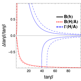
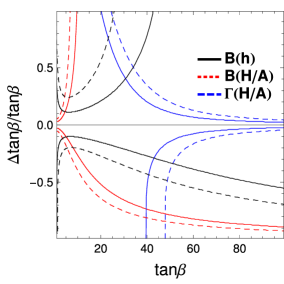
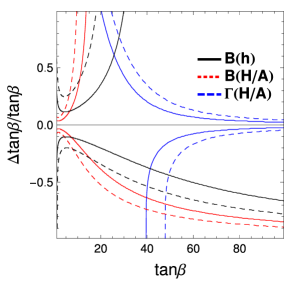
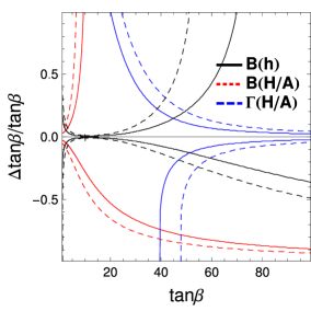
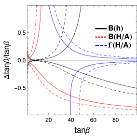
Figure 3: Sensitivities to the $\tan\beta$ measurement by the three methods in the Type-II THDM. From left to right, $\sin^{2}(\beta-\alpha)$ is taken to be $1$, $0.99$, and $0.98$, with $\cos(\beta-\alpha)\leq 0$. Estimated $\Delta\tan\beta/\tan\beta$ by using the branching ratio of $H/A\to b\bar{b}$ (red curves), the total width of $H/A$ (blue curves), and the branching ratio of $h\to b\bar{b}$ (black curves) are plotted as a function of $\tan\beta$. The solid curves stand for $1\sigma$ sensitivities, and the dashed curves for $2\sigma$. For $HA$ production, $m_{H}=m_{A}=200$ GeV with $\sqrt{s}=500$ GeV and ${\mathcal{L}}_{\rm int}=250~{}\text{fb}^{-1}$ are assumed. For the $h\to b\bar{b}$ measurement, $\Delta{\mathcal{B}}/{\mathcal{B}}=1.3\%$ ($1\sigma$) and $2.7\%$ ($2\sigma$) are used.

Figure 4: The same as FIG. 4, but for $\cos(\beta-\alpha)\geq 0$.

In FIG. 4, our numerical results for the three methods are shown. The results for $1\sigma$ (solid) and $2\sigma$ (dashed) sensitivities for the branching ratios, the total width of $H$ and $A$, and the branching ratio of $h$ are plotted in the red, blue and black curves, respectively. The parameter $\sin^{2}(\beta-\alpha)$ is set to be $1$ (left), $0.99$ (middle), and $0.98$ (right) with $\cos(\beta-\alpha)\leq 0$. The case with $\cos(\beta-\alpha)\geq 0$ is also shown in FIG. 4.

In the Type-II THDM, the three methods complementary cover the wide range of $\tan\beta$ values. In the SM-like limit (left panels of FIGs. 4 and 4), the method using the $h$ decay has no sensitivity to $\tan\beta$. But, for $\sin^{2}(\beta-\alpha)=0.99$, 0.98, there are certain $\tan\beta$ regions, from about 5 to 30$\sim$40, where it gives the best sensitivity among the three methods. The sensitivity for $\cos(\beta-\alpha)>0$ is better than that for $\cos(\beta-\alpha)<0$, because the former case has a large gradient $|d{\mathcal{B}}/d(\tan\beta)|$, as shown in FIG. 1. On the other hand, in the $\cos(\beta-\alpha)>0$ case, there is a two-fold ambiguity in determining $\tan\beta$ from the ${\mathcal{B}}_{bb}^{h}$. We expect that this ambiguity is resolved by using the other methods, or by measuring the branching ratios in the other $h$ decay modes, such like into $gg$ and $c\bar{c}$.

The sensitivity for the $h$ decay becomes worse for large $\tan\beta$, where ${\mathcal{B}}^{h}_{bb}$ is saturated at about 90% as shown in FIG. 1. We note that, however, such a large deviation in the decay branching ratios of $h$ should be constrained from the LHC data, where, e.g., the prediction of ${\mathcal{B}}(h\to ZZ^{*})$ can be different from that in the SM.

III.2 Sensitivity to $\tan\beta$ in the Type-X THDM

In the Type-X THDM, the sensitivities to $\tan\beta$ are evaluated similarly to the case in the Type-II THDM, but the decay mode of $\tau\tau$ is used instead of that of $b\bar{b}$. For $HA$ production, the acceptance for the $4\tau$ final state is estimated to be 50% (for details, see Appendix A). The detector resolution for the Breit-Wigner width in the invariant mass distribution of $\tau\tau$ ($M_{\tau\tau}$) is obtained with the use of the collinear approximation Ref:KTY , which is estimated to be $7$ GeV. The selection efficiency due to the mass window cut $M_{\tau\tau}\pm 10$ GeV is 30%. For the $h\to\tau\tau$ decay, expected accuracy of the measurement of the branching ratio at the ILC is $\Delta{\mathcal{B}}^{h}_{\tau\tau}/{\mathcal{B}}^{h}_{\tau\tau}=5\%$ (2%) in the $2\sigma$ ($1\sigma$) CL in the SM for $\sqrt{s}=250$ GeV and ${\mathcal{L}}_{\rm int}=250$ fb^-1 Ref:h-BR . We rescale them to the case in the Type-X THDM with certain values of $\sin^{2}(\beta-\alpha)$ and $\tan\beta$ taking into account the changes of the number of the signal events.

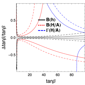
Figure 5: The same as FIG. 4, but $\tau\tau$ decay modes are used for the analysis in the Type-X THDM. From left to right, $\sin^{2}(\beta-\alpha)$ is taken to be $1$, $0.99$, and $0.98$, with $\cos(\beta-\alpha)\leq 0$. For ${\mathcal{B}}^{h}_{\tau\tau}$, $\Delta{\mathcal{B}}/{\mathcal{B}}=2\%$ ($1\sigma$) and $5\%$ ($2\sigma$) are assumed.

Figure 6: The same as FIG. 6, but for $\cos(\beta-\alpha)\geq 0$.

In FIGs. 6 and 6, the numerical results in the Type-X THDM are presented in the same manner as in FIGs. 4 and 4 in the Type-II case, respectively. With or without the assumption of $\sin(\beta-\alpha)=1$, the total width measurement of $H$ and $A$ is a useful probe for the large $\tan\beta$ regions. For the smaller $\tan\beta$ regions, the branching ratio measurement of $H$ and $A$ can probe $\tan\beta$ well. As noted in the Type-II case, the $h$ decay does not have a sensitivity to $\tan\beta$ in the SM-like limit (left panels). However, for $\sin(\beta-\alpha)=0.99$ and 0.98, ${\mathcal{B}}^{h}_{\tau\tau}$ measurement can give the best sensitivity for a wide range of $\tan\beta$ values. This is because the branching ratio of $h\to\tau\tau$ is about 10 times smaller than that of $h\to b\bar{b}$, and thus the saturation of the branching ratio for large $\tan\beta$ is relatively delayed as compared to the case in the Type-II THDM. This is also true for the branching ratios of $H/A\to\tau\tau$. In the $\cos(\beta-\alpha)>0$ case, the method using the $h$ decay has two-fold ambiguity to determine $\tan\beta$ from the ${\mathcal{B}}_{\tau\tau}^{h}$ measurement. This ambiguity is expected to be solved by using the other methods.

III.3 Sensitivity to $\tan\beta$ in the other types of the THDM

Here, we comments on the $\tan\beta$ measurements for the other types in the THDM. In the Type-I THDM, the Yukawa coupling constants are universally changed from those in the SM. In the SM-like limit, $\sin(\beta-\alpha)=1$, Yukawa interactions for $H$ and $A$ become weak for $\tan\beta>1$. As for the $\tan\beta$ measurement at the ILC, the method by using the total width of $H$ and $A$ is useless, because the absolute value of the decay width is too small as compared to the detector resolution. Without the SM-like limit, the branching ratio measurement of $H$ and $A$ using the fermionic decay modes may be difficult, because the bosonic decay modes $H\to WW$ and $A\to Zh$ become important. Furthermore, the decays of $h$ are almost unchanged from the SM because of no $\tan\beta$ enhancement. Thus, the $\tan\beta$ determination in the Type-I THDM seems to be difficult even at the ILC.

In the Type-Y THDM, the sensitivities to $\tan\beta$ at the ILC would be similar to those in the Type-II THDM, because the Yukawa interactions of the neutral scalar bosons with the bottom quarks are enhanced by $\tan\beta$ as the same way as those in the Type-II THDM.

IV Conclusion and discussion

We have studied the physics potential for the $\tan\beta$ determination at the ILC in the THDMs. In addition to the masses of the extra Higgs bosons, $\tan\beta$ and $\sin(\beta-\alpha)$ are important parameters in the THDM, which describe the electroweak symmetry breaking sector in the model. At the ILC, the parameter $\sin^{2}(\beta-\alpha)$ is determined very precisely. The branching ratios of the $h$ decay can also be measured precisely and independently of $\sin^{2}(\beta-\alpha)$. Since the Yukawa coupling constants of $h$ are modified if $\sin(\beta-\alpha)\neq 1$, the combination of these measurements can constrain $\tan\beta$. If $H$ and $A$ are light, measurements of the decay branching ratio and the total decay width can also probe $\tan\beta$.

In this paper, we have studied the sensitivities of the $\tan\beta$ measurements using these observables in the Type-II and Type-X THDMs. In the Type-II THDM, the down-type quark and the lepton Yukawa interactions of $H$ and $A$ largely depend on $\tan\beta$. Since the masses of $H$ and $A$ have been strongly constrained by the LHC data and the flavor data, direct searches of them and the precision measurements of their properties should require relatively high collision energy at the ILC. On the other hand, the $h$ decay can explore $\tan\beta$ if $\sin(\beta-\alpha)\neq 1$ through the precision measurement of its branching ratios.

In the Type-X THDM, only the leptonic Yukawa interactions of $H$ and $A$ are enhanced for the large $\tan\beta$ regions. Since they have less interaction with quarks, a severe bound from the LHC data and the flavor data can be evaded. Therefore, $H$ and $A$ can be light enough to be produced at the ILC. If they are light, $\tan\beta$ can be determined by the direct measurement of their properties at the ILC. We have compared the sensitivities to $\tan\beta$ using these measurements and the $h$ decay. We find that the precision study of the branching ratios in the $h$ decay is very useful to determine $\tan\beta$ in the Type-X THDM for the wide range of parameter space.

In conclusion, we have studied the methods of the $\tan\beta$ measurement in general THDMs at linear colliders. In addition to the methods previously proposed by using the extra Higgs bosons, we have discussed the method which uses the precision measurement of the $h$ decay. We have found that $\tan\beta$ can be determined very well in a wide range of $\tan\beta$ values at the ILC by combining these methods.

Appendix A Simulation detail in $HA$ production

In this appendix, we present our estimation of the efficiencies for the $4b$ and $4\tau$ events and the resolution of the width in the $bb$ and $\tau\tau$ invariant mass distributions in the $e^{+}e^{-}\to HA$ process. The simulation is performed by using the hadron-level events with Pythia Ref:PYTHIA and FastJet Ref:FastJet for jet clustering.

For each event, we collect the final state particles with $|\eta|<2$ where the pseudorapidity is $\eta=\frac{1}{2}\ln\frac{1+\cos\theta}{1-\cos\theta}$, and $\theta$ is the polar angle of particle’s momentum in the laboratory frame. For charged particles, a cut on the transverse momentum, $p_{T}>300$ MeV, is also applied. The momenta are smeared by Gaussian distributions with $\sigma_{E}/E=15\%/\sqrt{(E~{}[{\rm GeV}])}+1\%$ for photons, $\sigma_{E}/E=40\%/\sqrt{(E~{}[{\rm GeV}])}+2\%$ for neutral hadrons, and $\sigma_{p}/p_{T}=10^{-4}\times(p_{T}~{}[{\rm GeV}])+0.1\%$ for charged particles, where $\sigma$’s are a dispersion of each distribution. Then, the particles are clustered into four by using the Durham-$k_{T}$ algorithm Ref:KT . The cluster is identified as $\gamma$, if the cluster contains only $\gamma$’s. The cluster is identified as $e^{\pm}$ or $\mu^{\pm}$, if the cluster contains one and only one $e^{\pm}$ or $\mu^{\pm}$ and its $p_{T}$ is more than 95% of the cluster. Otherwise, we identify the cluster as a jet. The jet is tagged as a $\tau$-jet, if the cluster contains one or three charged particles and the sum of $p_{T}$ of particles inside the $R=0.15$ cone is more than 95% of $p_{T}$ of the cluster. The jet which has $B$-hadrons in the decay history of its constituent particles is tagged as a $B$-jet with the probability of 65%. The other jet which has $D$-hadrons in the decay history of its constituent particles is tagged as a $B$-jet with the probability of 1%. Other jets are tagged as $B$-jets with the probability of 0.1%.

For the $4b$ events, we take the events with four $B$-jets or three $B$-jets plus one jet. With the above $B$-tagging probabilities, we find that the efficiency of finding the $4b$ events is about 50%. Absolute values of the 4-momenta of the four jets are rescaled so that the sum of the 4-jet energy is equal to the collision energy and the sum of the 3-momenta of the four jets vanishes. Then, the di-$B$-jet invariant mass $M_{BB}$ can be reconstructed, where the pairs of the di-$B$-jet are chosen such that the difference of the two invariant masses is minimal. By fitting the distribution in a Breit-Wigner form, we get the width $\Gamma_{\rm res}\simeq 11$ GeV, which is assumed to be the systematical resolution of the width measurement. We note that this value is roughly twice of that used in Ref. Ref:TanB .

For the $4\tau$ events, we take the events which contain four $\tau$-jets or three $\tau$-jets with one charged lepton or two $\tau$-jets with two same-sign charged leptons. These signatures are expected to have small SM background contributions. The efficiency of finding the $4\tau$ events is about 50%. Then, the 4-momenta of 4$\tau$’s can be reconstructed by rescaling the absolute values of the 4-momenta of the four objects so that the energy sum is equal to the collision energy and the sum of the 3-momenta vanishes. The Di-$\tau$ invariant mass $M_{\tau\tau}$ is reconstructed, where the pairs of di-$\tau$ are chosen such that the difference of the two invariant masses is minimal with avoiding the same-sign charged leptons to be paired. By fitting the distribution in a Breit-Wigner form, we get the width $\Gamma_{\rm res}\simeq 7$ GeV. We note that the $\tau$-jet momentum is measured in a good accuracy by the charged-tracks, while the accuracy of the collinear approximation in the $\tau$ decays becomes a dominant source of the systematical resolution of the width measurement.

References

- (1) ATLAS Collaboration, Phys. Lett. B 716, 1 (2012).
- (2) CMS Collaboration, Phys. Lett. B 716, 30 (2012).
- (3) ATLAS Collaboration, Report No. ATLAS-CONF-2013-034.
- (4) CMS Collaboration, Report No. CMS-PAS-HIG-12-045.
- (5) J. F. Gunion, H. E. Haber, G. Kane and S. Dawson, The Higgs Hunter’s Guide (Frontiers in Physics series, Addison-Wesley, Reading, MA, 1990).
- (6) S. L. Glashow, S. Weinberg, Phys. Rev. D15 (1977) 1958.
- (7) G. C. Branco, P. M. Ferreira, L. Lavoura, M. N. Rebelo, M. Sher and J. P. Silva, Phys. Rept. 516, 1 (2012).
- (8) H. E. Haber and G. L. Kane, Phys. Rept. 117, 75 (1985).
- (9) A. Djouadi, Phys. Rept. 459, 1 (2008).
- (10) E. Ma, Mod. Phys. Lett. A 17, 535 (2002); E. Ma and D. P. Roy, Nucl. Phys. B 644, 290 (2002).
- (11) M. Aoki, S. Kanemura and O. Seto, Phys. Rev. Lett. 102, 051805 (2009); M. Aoki, S. Kanemura and O. Seto, Phys. Rev. D 80, 033007 (2009); M. Aoki, S. Kanemura and K. Yagyu, Phys. Rev. D 83, 075016 (2011).
- (12) H. -S. Goh, L. J. Hall and P. Kumar, JHEP 0905, 097 (2009).
- (13) Y. Bai, V. Barger, L. L. Everett and G. Shaughnessy, arXiv:1212.5604 [hep-ph].
- (14) J. Cao, P. Wan, L. Wu and J. M. Yang, Phys. Rev. D 80, 071701 (2009).
- (15) G. Aad et al. [ATLAS Collaboration], JHEP 1302, 095 (2013).
- (16) CMS Collaboration, Report No. CMS-PAS-HIG-12-050.
- (17) Y. Bai, V. Barger, L. L. Everett and G. Shaughnessy, arXiv:1210.4922 [hep-ph]; A. Celis, V. Ilisie and A. Pich, arXiv:1302.4022 [hep-ph]; C. -W. Chiang and K. Yagyu, arXiv:1303.0168 [hep-ph]; P. P. Giardino, K. Kannike, I. Masina, M. Raidal and A. Strumia, arXiv:1303.3570 [hep-ph]; C. -Y. Chen, S. Dawson and M. Sher, arXiv:1305.1624 [hep-ph]; O. Eberhardt, U. Nierste and M. Wiebusch, arXiv:1305.1649 [hep-ph]; N. Craig, J. Galloway and S. Thomas, arXiv:1305.2424 [hep-ph].
- (18) M. Ciuchini, E. Franco, G. Martinelli, L. Reina, L. Silvestrini, Phys. Lett. B334 (1994) 137-144; M. Ciuchini, G. Degrassi, P. Gambino, G. F. Giudice, Nucl. Phys. B527 (1998) 21-43; F. Borzumati, C. Greub, Phys. Rev. D58 (1998) 074004; P. Gambino, M. Misiak, Nucl. Phys. B611 (2001) 338-366.
- (19) M. Misiak, H. M. Asatrian, K. Bieri, M. Czakon, A. Czarnecki, T. Ewerth, A. Ferroglia, P. Gambino et al., Phys. Rev. Lett. 98 (2007) 022002.
- (20) W. -S. Hou, Phys. Rev. D48 (1993) 2342-2344; Y. Grossman, Z. Ligeti, Phys. Lett. B332 (1994) 373-380; Y. Grossman, H. E. Haber, Y. Nir, Phys. Lett. B357 (1995) 630-636.
- (21) W. Hollik, T. Sack, Phys. Lett. B284 (1992) 427-430; M. Krawczyk, D. Temes, Eur. Phys. J. C44 (2005) 435-446.
- (22) V. D. Barger, J. L. Hewett, R. J. N. Phillips, Phys. Rev. D41 (1990) 3421; Y. Grossman, Nucl. Phys. B426 (1994) 355-384.
- (23) M. Aoki, S. Kanemura, K. Tsumura, K. Yagyu, Phys. Rev. D80 (2009) 015017.
- (24) S. Su and B. Thomas, Phys. Rev. D 79, 095014 (2009).
- (25) H. E. Logan and D. MacLennan, Phys. Rev. D 79, 115022 (2009).
- (26) H. Ono and A. Miyamoto, Eur. Phys. J. C 73, 2343 (2013).
- (27) J. Brau, P. Grannis, M. Harrison, M. Peskin, M. Ross and H. Weerts, arXiv:1304.2586 [physics.acc-ph].
- (28) M. E. Peskin, arXiv:1207.2516 [hep-ph].
- (29) V. D. Barger, T. Han and J. Jiang, Phys. Rev. D 63, 075002 (2001); J. F. Gunion, T. Han, J. Jiang and A. Sopczak, Phys. Lett. B 565, 42 (2003).
- (30) G. Aad et al. [ATLAS Collaboration], JHEP 1206, 039 (2012); arXiv:1302.3694 [hep-ex].
- (31) S. Kanemura, Y. Okada, E. Senaha and C. -P. Yuan, Phys. Rev. D 70, 115002 (2004).
- (32) S. Kanemura, T. Kubota and E. Takasugi, Phys. Lett. B 313, 155 (1993); A. G. Akeroyd, A. Arhrib and E. -M. Naimi, Phys. Lett. B 490, 119 (2000).
- (33) D. Toussaint, Phys. Rev. D 18, 1626 (1978);
- (34) S. Bertolini, Nucl. Phys. B 272, 77 (1986).
- (35) W. Hollik, Z. Phys. C 32, 291 (1986); Z. Phys. C 37, 569 (1988).
- (36) S. Kanemura, Y. Okada, H. Taniguchi and K. Tsumura, Phys. Lett. B 704, 303 (2011).
- (37) ILD Concept Group, The International Large Detector: Letter of Intent, KEK Report 2009-6.
- (38) A. Yamamoto, presentation at the Asian Physics and Software Meeting, June, 2012.
- (39) S. Kanemura, K. Tsumura and H. Yokoya, Phys. Rev. D 85, 095001 (2012); Proceedings for LCWS11, 26-30 Sep 2011. Granada, Spain, arXiv:1201.6489 [hep-ph].
- (40) T. Sjostrand, S. Mrenna and P. Z. Skands, JHEP 0605 (2006) 026.
- (41) M. Cacciari, G. P. Salam and G. Soyez, Eur. Phys. J. C 72 (2012) 1896.
- (42) S. Catani, Y. L. Dokshitzer, M. Olsson, G. Turnock and B. R. Webber, Phys. Lett. B 269 (1991) 432.