Anti-persistent behavior of defects in a lyotropic liquid crystal during annihilation

Abstract

We report on the dynamical behavior of defects of strength $s=\pm\,1/2$ in a lyotropic liquid crystal during the annihilation process. By following their positions using time resolved polarizing microscopy technique, we present statistically significant evidence that the relative velocity between defect pairs is Gaussian distributed, anti-persistent and long-range correlated. We further show that simulations of the Lebwohl-Lasher model reproduce quite well our experimental findings.

Introduction - The understanding of ordering processes in condensed matter has been the focus of considerable research over the last decades chuang ; turok ; finn ; yurke ; toyoki ; zapotocky ; marshall ; dutta ; rey ; oliveira ; oliveira2 . One of the main aspects of the ordering process is the dynamical behavior of defects present in the material. Topological defects appear in several systems that present some kind of ordering kibble ; charlier ; figueiras ; petit ; abu ; carvalho . Alloys hamad , semiconductors emtsev , polymers quarti and liquid crystals pasini ; mukai are just a few examples. In particular, optical textures of liquid crystals chandra ; degennes ; figueiredo_book are known to be an excellent system for studying the dynamical behavior of defects. In fact, there are several studies on the annihilation dynamics of defects in liquid crystals employing thermotropics marshall ; cypt ; mendez ; minoura , thermotropic polyester materials shiwaku ; ding ; wang and lyotropic renato . Moreover, the experimental analysis of annihilation processes has also motivated many numerical simulations yurke ; zapotocky ; oliveira ; svensek ; svetec . One of the most striking results of these studies is the scaling law in the relative distance $D(t)$ between defect and anti-defect during the annihilation process, that is, $D(t)\sim t^{\alpha}$, where $t$ is the remaining time for the annihilation and $\alpha$ is the power law exponent. It is also known that defect and anti-defect present an anisotropic behavior when approaching each other, the defect usually moves faster than the anti-defect toth ; toth2 ; svensek2 ; oswald ; blanc . This last aspect has been recently addressed both, experimentally and numerically, by Dierking et al. dierking2 , for umbilical defects in a thermotropic liquid crystal under applied electric field.

It is surprising that almost no attention has been paid to understand higher order properties of defect trajectories. In this brief report, we fill some of these lacunas by investigating correlational aspects and the velocity distribution of the defects. Specially, we present statically significant evidence that the relative velocity between defects pairs in a lyotropic liquid crystal is Gaussian distributed, anti-persistent and long-range correlated. Furthermore, we show that these behaviors also appear in our numerical simulations of the Lebwohl-Lasher model leblas by using a Langevin approach yurke ; bac . In following, we present the experimental setup used to obtain the liquid crystal textures, the image technique employed to follow the defect motions, the analysis of the experimental data, the Lebwhol-Lasher model used for reproducing our experimental findings and, finally, a summary of our results.

Experimental Setup - The lyotropic system we have studied is a mixture of potassium laurate (KL $\rightarrow$ 27.49 wt%), decanol (DeOH $\rightarrow$ 6.24 wt%) and distilled and deionized water (H₂O $\rightarrow$ 66.27 wt%). At these concentrations, our lyotropic system presents an isotropic $\to$ nematic transition at $\approx 40^{\circ}$ Celsius. Furthermore, Mukai et al. mukai have observed the defects in lyotropic systems are more stable than those ones obtained in thermotropic liquid crystals. We have made a series of 8 samples of this lyotropic system by using sealed films in flat capillaries (100 $\mu$m thick by 2 mm width by 2 cm length). These samples were placed in a polarized light microscope coupled with a hostage (INSTEC model HCS302), enabling the precise control of the temperature with ${0.01}^{\circ}$ Celsius accuracy. In order to produce the defects, we have promoted a spontaneous symmetry breaking mukai ; kleman by raising the temperature of the sample to $50^{\circ}$ Celsius (isotropic region) and suddenly changing it to $25^{\circ}$ Celsius (nematic region). After this temperature change, we first observed colorful domains, and next ($\approx 5$ hours later) the defects become visible. The defects observed in these samples are characterized by a strength $s=\pm 1/2$, since they have two dark branches from a dark point. We thus started to capture snapshots of the evolution of so called “Schlieren” texture dierking_book ; figueiredo_book at a sample rate of 15 pictures by hour until the vanishing of all defects in the sample ($\approx 20$ hours after the phase transition). Figure 1(a) shows characteristic textures where the dark branches correspond to areas where the director $\vec{n}$ is perpendicular or parallel to one of the polarizers, while in the bright regions represent areas where the director $\vec{n}$ is tilted compared with the polarizers. The defect is exactly located between the junction of two dark branches, where the orientation of director $\vec{n}$ is not defined. In general, there appear about 20 pairs of defects across the sample and usually 5 of them fall within the microscope region of view.

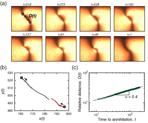
Figure 1: (Color online) Annihilation process of defects in our lyotropic system. (a) Typical evolution of textures during the annihilation. The $t$ value (above of each image) stands for the remaining time (in minutes) to the annihilation. The square represents the initial position of the defect and the circle is the same for the anti-defect. The arrow indicates the relative distance between the defect and the anti-defect. (b) The trajectories of the two defects obtained via the Lucas-Kanade algorithm Lucas . The distance units are given in pixels. (c) The scaling law describing the relative distance between the defects, that is, $D(t)\propto t^{0.4}$.

Data analysis - By using sequences of textures of the annihilation process, we track the motion of the defect pairs using the Lucas-Kanade algorithm Lucas . In this algorithm, we give the initial positions of a defect pair in the first image and, it automatically assigns the position of the defects in the subsequent images. Figure 1(b) shows an example of trajectories of a defect (upper curve) and an anti-defect (bottom curve). We observe that the defect moves about twice the distance of the anti-defect, similarly to the previous-mentioned behavior of umbilical defects in a thermotropic liquid crystal dierking2 . We have tracked the evolution of defects in 49 annihilations. For sake of definition, let $\vec{r}_{+}(t)=(x_{+}(t),y_{+}(t))$ be the position vector of the defect and $\vec{r}_{-}(t)=(x_{-}(t),y_{-}(t))$ represents the same for the anti-defect. Here, we focus our analysis on the relative distance in a pair of defects $D(t)=\|\vec{r}_{+}(t)-\vec{r}_{-}(t)\|$ and also on the relative velocity $V(t)=\frac{D(t+dt)-D(t)}{dt}$. Figure 1(c) shows the scaling law that characterizes the evolution of the relative distance, that is, $D(t)\sim t^{\alpha}$, with $\alpha=0.4$ in this case (see Ref. renato for a more detailed study of this scaling law).

We start our analysis by asking whether the probability distribution of the relative velocities follows a particular functional form. Figure 2(a) shows an example of time series of the relative velocities. Note that we have employed normalized velocities, that is, $\nu(t)=[V(t)-\langle V(t)\rangle]/\sigma(t)$, where $\sigma^{2}(t)=\langle[V(t)-\langle V(t)\rangle]^{2}\rangle$ and $\langle\dots\rangle$ stands for the average value. We observe that the normalized velocities fluctuate around zero with a variance that seems to not depend on the time $t$. We have evaluated the cumulative distributions of these velocities for all the 49 experimental trajectories, as shown in Figure 2(b). We note that the distributions exhibit a good collapse and a profile that is quite similar to the Gaussian distribution of zero mean and unitary variance. In fact, the Kolmogorov-Smirnov test cannot reject the Gaussian hypothesis (on a significance level of 95%) in $\sim 80$% of the cases. In addition, we remark that the Gaussian distribution describes almost perfectly the average values of these distributions (squares in Fig. 2(b)).

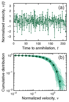
Figure 2: (Color online) Statistics of the relative velocity between pairs of defects in our lyotropic system. (a) Typical time series of the normalized relative velocities $\nu(t)$. (b) Cumulative distributions of $\nu(t)$ for all the 49 experimental trajectories. The continuous lines represent both the positive and negative (taking the absolute values) tails, while the squares are average values over all distributions. The error bars are 95% confidence intervals obtained via bootstrapping bootstrap . We note a good collapse of the empirical distributions and also that these distributions are quite similar to the Gaussian distribution of zero mean and unitary variance (dashed line).

Another interesting question is whether there is long-range memory in the evolution of the velocities $\nu(t)$. To investigate this hypothesis, we have analyzed the time series of the normalized velocities via detrended fluctuation analysis (DFA) peng ; bunde . In this analysis, we first define the profile $Y(i)=\sum_{k=1}^{i}\nu(t_{k})-\langle\nu(t_{k})\rangle$ and, next, we cut $Y(i)$ into $N_{n}=N/n$ nonoverlapping segments of size $n$, where $N$ is the length of the series (typically $N\approx 200$ in our study). For each of these segments, we fit a polynomial trend (here a polynomial of degree 1), which is subtracted from $Y(i)$, defining $Y_{n}(i)=Y(i)-p_{j}(i)$, where $p_{j}(i)$ is the local trend in the $j$-th segment. We thus evaluate the root-mean-square fluctuation function $F(n)=[\frac{1}{N_{n}}\sum_{j=1}^{N_{n}}\langle Y_{n}(i)^{2}\rangle_{j}]^{1/2}$, where $\langle Y_{n}(i)^{2}\rangle_{j}$ is the mean-square value of $Y_{n}(i)$ over the data in the $j$-th segment. For self-similar time series, $F(n)$ should display a power law dependence on the time scale $n$, that is, $F(n)\sim n^{h}$, where $h$ is the Hurst exponent. In our case, the DFA is shown in Fig. 3. We have found that the average value of the Hurst exponents over all experimental results is $0.43$, where the lower and upper bounds of the 95% confidence interval are $0.40$ and $0.46$. Our results thus confirm the existence of long-range correlations in the evolution of $\nu(t)$. Moreover, since $h<0.5$, the velocities present an anti-persistent beaviour where the alternation between large and small values of $\nu(t)$ occurs more frequently than by chance.

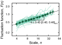
Figure 3: (Color online) Long-range and anti-persistent correlations in the relative velocities in pairs of defects in our lyotropic system. (a) Detrended fluctuation analysis (DFA) of the normalized velocities $\nu(t)$. We show the fluctuation functions $F(n)$ versus the scale $n$ for all the 49 experimental results (continuous lines) and their average values (squares). The error bars are 95% confidence intervals obtained via bootstrapping bootstrap . We have found the mean value of the Hurst exponent to be $h=0.43$ and the dashed line is a power law with this exponent. The values between brackets represent the 95% confidence interval for $h$ obtained via bootstrapping. We remark the anti-persistent behavior of the velocities indicated by $h<0.5$.

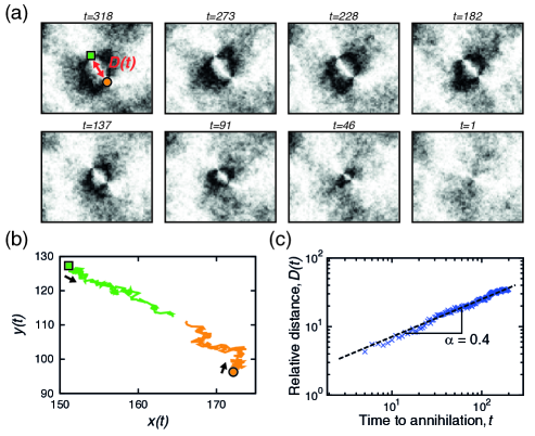
Figure 4: (Color online) Annihilation process of defects obtained from the simulation of the Lebwohl-Lasher model. (a) Snapshots of a simulated texture of a defect pair in the course annihilation. The $t$ value above each image represents the number of iterations of the Lebwohl-Lasher model until the annihilation and the square and circle are the initial positions of the defects. (b) Typical trajectories of the simulated evolution of a defect pair obtained via the Lucas-Kanade algorithm Lucas . (c) The scaling law describing the relative distance between the simulated defects. Analogously to the experimental case, we have found $D(t)\propto t^{0.4}$.

Modeling - We now focus on modeling the previous experimental results. To this end, we have considered the well stablished Lebwohl-Lasher model leblas ; bac using a Langevin approach yurke . Differently from the model $XY$ model yurke , which produces defects of strength $s=\pm 1$, the planar Lebwohl-Lasher model showed to be able of generating topological defects with the same strength of those ones observed in our lyotropic systems, that is, $s=\pm 1/2$. This model consists of $M\times M$ spins located in a square lattice with periodic boundary conditions. The orientation of the $i$-th spin is given by the angle $\phi_{i}(\tau)$, which evolves according the Langevin-like equation yurke

$$\phi_{i}(\tau+\Delta t)=\phi_{i}(\tau)-\Delta\tau\left\{2\,\pi\,c_{\,T}\,\eta_{i}+\frac{1}{2}\sum_{j}\,\sin[\,2(\phi_{i}(\tau)-\phi_{j}(\tau))]\right\}\,.$$

Here, the sum over $j$ is carried out over the eight nearest neighbors of $i$, $\eta_{i}$ is a random number with uniform distribution ranging from -0.5 to 0.5, $c_{\,T}$ is a model parameter for adjusting the noise amplitude and, $\Delta t=0.05$ is the time increment. In our simulations, we have used $M=250$ and a random initial configuration, where $\phi_{i}(0)$ was chosen from a uniform distribution between $0$ and $2\pi$. This condition is analogous to the isotropic phase displayed by our lyotropic system at $50^{\circ}$ Celsius. Also, we have chosen $c_{\,T}=0.7$ because this value is below the corresponding one of the phase transition ($c_{\,T}\approx 2.6$); as pointed out previously, the temperature of $25^{\circ}$ Celsius is below the isotropic $\to$ nematic transition of our lyotropic system. The simulations typically ran up to $\tau=5\times 10^{3}$ and the equivalent to lyotropic textures were obtained by building images where the gray intensity of $i$-th pixel is proportional to $\sin^{2}(2\,\phi_{i})$. Figure 4(a) shows snapshots of one of the 49 annihilation processes obtained through our simulations.

Once we have the simulated textures of the annihilation process (Fig. 4(a)), we proceed as in the experimental case, that is, we applied the Lucas-Kanade algorithm for tracking the positions of the defects (Fig. 4(b)) and evaluated the relative distance $D(t)$. As shown in Fig. 4(c), Lebwohl-Lasher model also generates a power law evolution for the distance $D(t)$ with the same exponent ($\alpha=0.4$) obtained for the lyotropic system (Fig. 1(a)). Remarkably, the model reproduces quite well the Gaussian distribution of the normalized velocities $\nu(t)$, as shown in Fig. 5(a) and 5(b), and the anti-persistent and long-range behaviors of $\nu(t)$, as shown in Fig. 6. Regarding this last point, we note that the average value of the Hurst exponent $h$ is slightly smaller in simulated case than in the experimental one. However, from the statistical point of view, we cannot reject the hypothesis of equality of both means since there is overlapping in their confidence intervals.

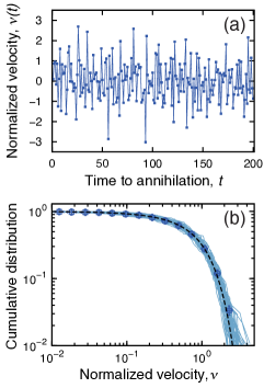
Figure 5: (Color online) Statistics of the relative velocities in pairs of defects obtained through the simulation of the Lebwohl-Lasher model. (a) Typical time series of the normalized relative velocities $\nu(t)$. (b) Cumulative distribution of $\nu(t)$ for all the 49 simulated trajectories. The continuous lines represent both the positive and negative (taking the absolute values) tails, while the squares are the averaged values over all distributions. The error bars are 95% confidence intervals obtained via bootstrapping bootstrap . Similarly to experimental case, we have found a good collapse of the distribution and also a good agreement with the Gaussian distribution of zero mean and unitary variance (dashed line). The the Kolmogorov-Smirnov test cannot reject the Gaussian hypothesis (on a significance level of 95%) in $\sim 90$% of the cases.

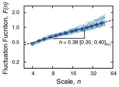
Figure 6: (Color online) Anti-persistent and long-range correlations in the relative velocities between defects obtained through the simulation of the Lebwohl-Lasher model. (a) Detrended fluctuation analysis (DFA) of the normalized velocities $\nu(t)$. We show the fluctuation functions $F(n)$ versus the scale $n$ for all the 49 simulated results (continuous lines) and their average values (squares). The error bars are 95% confidence intervals obtained via bootstrapping bootstrap . Similarly to experimental case, the mean value of the Hurst exponent is $h=0.38$ and the dashed line is a power law with this exponent. The values between brackets represent the 95% confidence interval for $h$ obtained via bootstrapping. Note the existence of overlap in the confidence intervals obtained for the experimental results and the simulated ones.

Summary - We have thus studied the annihilation dynamics of defects in a lyotropic system. Our analysis revealed that, in addition to the power law behavior of the relative distance $D(t)$, the motion of these defects are characterized by relative velocities $\nu(t)$ that are Gaussian distributed and present long-range correlations with an average Hurst exponent of $h=0.43$. This smaller than $1/2$ value of $h$ indicates that changes between small and large values of $\nu(t)$ occur much more frequently than by chance. In order to model the experimental results, we have employed the Lebwohl-Lasher model due its simplicity and ability of generating the same type of topological defects present in our lyotropic system. The results obtained from this model showed to be amazingly similar to the experimental ones. We further believe that our work prompt new questions such as whether this anti-persistent behavior is a universal characteristic of the annihilation or it is a system-specific behavior.

- (1) I. Chuang, R. Durrer, N. Turok, and B. Yurke, Science 251, 1336 (1991).
- (2) I. Chuang, N. Turok, and B. Yurke, Phys. Rev. Lett. 66, 2472 (1991).
- (3) A. N. Pargellis, P. Finn, J. W. Goodby, P. Panizza, B. Yurke, and P. E. Cladis, Phys. Rev. A 46, 7765 (1992).
- (4) B. Yurke, A. N. Pargellis, T. Kovacs, and D. A. Huse, Phys. Rev. E 47, 1525 (1993).
- (5) H. Toyoki, Phys. Rev. E 47, 2558 (1993).
- (6) M. Zapotocky, P. M. Goldbart, and N. Goldenfeld, Phys. Rev. E 51, 1216 (1995).
- (7) I. Dierking, O. Marshall, J. Wright, and N. Bulleid, Phys. Rev. E 71, 061709 (2005).
- (8) S. Dutta and S. K. Roy, Phys. Rev. E 71, 026119 (2005).
- (9) N. M. Abukhdeir and A. D. Rey, New Journal of Physics 10, 063025 (2008).
- (10) B. F. de Oliveira, P. P. Avelino, F. Moraes, and J. C. R. E. Oliveira, Phys. Rev. E 82, 041707 (2010).
- (11) P. P. Avelino, F. Moraes, J. C. R. E. Oliveira, and B. F. de Oliveira, Soft Matter 7, 10961 (2011).
- (12) T. W. B. Kibble, J. Phys. A - Math. and Gen. 9, 1378 (1976).
- (13) J. C. Charlier, T. W. Ebbesen, and P. Lambin, Phys. Rev. B 53, 11108 (1996).
- (14) C. Figueiras and B. F. de Oliveira, Annalen Der Physik 523, 898 (2011).
- (15) N. Petit-Garrido, R. P. Trivedi, J. Ignes-Mullol, J. Claret, C. Lapointe, F. Sagues, and I. I. Smalyukh, Phys. Rev. Lett. 107, 177801 (2011).
- (16) N. Abu-Libdeh and D. Venus, Phys. Rev. B 84, 094428 (2011).
- (17) J. Carvalho, C. Furtado, and F. Moraes, Phys. Rev. A 84, 032109 (2011).
- (18) N. T. Mahmoud, J. M. Khalifeh, B. A. Hamad, and A. A. Mousa, Intermetallics 33, 33 (2013).
- (19) N. Y. Arutyunov, M. Elsayed, R. Krause-Rehberg, V. V. Emtsev, G. A. Oganesyan, and V. V. Koziovski, J. Phys.: Condens. Matter 25, 035801 (2013).
- (20) C. Quarti, A. Milani, and C. Castiglioni, J. Phys. Chem. B 117, 706 (2013).
- (21) H. Mukai, P. R. G. Fernandes, B. F. de Oliveira, and G. S. Dias, Phys. Rev. E 75, 061704 (2007).
- (22) Y. K. Murugesan, D. Pasini, and A. D. Rey, Soft Matter 9, 1054 (2013).
- (23) S. Chandrasekhar, Liquid Crystals (Cambridge University Press, Cambridge, 1980).
- (24) P. G. de Gennes and J. Prost, The Physics of Liquid Crystals, 2nd ed. (Clarendon, Oxford, 1995).
- (25) A. M. Figueiredo, S. A. Salinas, The Physics of Lyotropic Liquid Crystals: Phase Transitions and Structural Properties (Oxford, New York, 2005).
- (26) I. Chuang, B. Yurke, A. N. Pargellis, and N. Turok, Phys. Rev. E 47, 3343 (1993).
- (27) A. N. Pargellis, J. Mendez, M. Srinivasarao, and B. Yurke, Phys. Rev. E 53, R25 (1996).
- (28) K. Minoura, Y. Kimura, K. Ito, and R. Hayakawa, Mol. Cryst. Liq. Cryst. 302, 345 (1997).
- (29) T. Shiwaku, A. Nakai, H. Hasegawa, and T. Hashimoto, Macromolecules 23, 1590 (1990).
- (30) D. K. Ding and E. L. Thomas, Mol. Cryst. Liq. Cryst. 241, 103 (1994).
- (31) W. Wang, T. Shiwaku, and T. Hashimoto, J. Chem. Phys. 108, 1618 (1998).
- (32) R. R. Guimarães, R. S. Mendes, P. R. G. Fernandes, and H. Mukai, Annihilation dynamics of stringlike topological defects in a nematic lyotropic liquid crystal (2013, submitted).
- (33) D. Svenšek and S. Žumer, Phys. Rev. E 66, 021712 (2002).
- (34) M. Svetec, S. Kralj, Z. Bradač, and S. Žumer, Eur. Phys. J. E 20, 71 (2006).
- (35) G. Tóth, C. Denniston, and J. M. Yeomans, Phys. Rev. Lett. 88, 105504 (2002).
- (36) G. Tóth, C. Denniston, and J. M. Yeomans, Phys. Rev. E 67, 051705 (2003).
- (37) D. Svenšek and S. Žumer, Phys. Rev. Lett. 90, 155501 (2003).
- (38) P. Oswald and J. Ignés-Mullol, Phys. Rev. Lett. 95, 027801 (2005).
- (39) C. Blanc, D. Svenšek, S. Žumer, and M. Nobili, Phys. Rev. Lett. 95, 097802 (2005).
- (40) I. Dierking, M. Ravnik, E. Lark, J. Healey, G. P. Alexander, and J. M. Yeomans, Phys. Rev. E 85, 021703 (2012).
- (41) P. A. Lebwohl and G. Lasher, Phys. Rev. A 6, 426 (1972).
- (42) C. Goze, R. Paredes, C. Vásquez, E. Medina, and A. Hasmy, Phys. Rev. E 63, 042701 (2001).
- (43) O. D. Lavrentovich and M. Kleman, Chirality in Liquid Crystals (Springer, New York, 2001).
- (44) I. Dierking, Textures of Liquid Crystals (Wiley-VCH, Weinheim, 2003).
- (45) B. D. Lucas and T. Kanade, Proceedings of the 1981 DARPA Imaging Understanding Workshop, 121 (1981).
- (46) B. Efron and R. Tibshirani, An Introduction to the Bootstrap (Chapman & Hall, New York, 1993).
- (47) C. K. Peng, S. V. Buldyrev, S. Havlin, M. Simons, H. E. Stanley, and A. L. Goldberger, Phys. Rev. E 49, 1685 (1994).
- (48) J. W. Kantelhardt, E. Koscielny-Bunde, H. H. A. Rego, S. Havlin, and A. Bunde, Physica A 295, 441 (2001).