Heavy-to-light chromomagentic matrix element

Abstract

We report the computation of the matrix element of the chromomagnetic operator of the flavour changing neutral current (FCNC)-type between a $B$- or $D$-meson state and a light hadron and off-shell photon. The computation is carried out by using the method of light-cone sum rules (LCSR). It is found that the matrix element exhibits a large strong phase for which we give a long distance interpretation. The analytic structure of the correlation function in use admits a complex anomalous threshold on the physical sheet, the meaning and handling of which within the sum rule approach is discussed. We compare our results to QCD factorisation for which spectator photon emission is end-point divergent.

1 Introduction

The chromomagnetic operator of the $b\to s$-type is defined as follows:

$$\tilde{\cal O}_{8}^{(^{\prime})}=\bar{s}\sigma_{\mu\nu}G_{a}^{\mu\nu}\frac{\lambda^{a}}{2}(1\pm\gamma_{5})b\;.$$ (1)

In the effective Hamiltonian ${\cal H}^{\rm eff}_{b\to s}=\,kG_{F}C_{8}\,[m_{b}(m_{s})\tilde{\cal O}_{8}]+..$, there is an additional factor of $m_{b}(m_{s})$, whose origin can be understood from the minimal flavour symmetry of the Standard Model (SM). The operator is therefore effectively of mass dimension six and thus on the same footing as the four-Fermi interactions.

The motivation for our work [1] is twofold: first, to provide an estimate of the chromomagnetic matrix element; and second, to compare it with the QCD factorisation (QCDF) calculation. The matrix element is of importance for isospin asymmetries [2, 3, 4, 5, 6], as the photon can be emitted from the spectator quark, and for testing for weak phases in $C_{8}^{(^{\prime})}$ [7, 8], which may be related to the relatively large direct CP-violation in $D^{0}\to\pi^{+}\pi^{-}/K^{+}K^{-}$ [10]. The comparison with QCDF is not natural as LCSR are not tailored around the heavy quark expansion and contain additional contributions not inherent in the QCDF calculation. Possibly the most surprising outcome of our investigations is the appearance of a complex anomalous threshold on the physical sheet in the correlation function used to extract the matrix element.

2 Definitions and computation

We aim to compute the following matrix element

$${\cal A}^{*\rho}(V) = \langle\gamma^{*}(q,\rho)V(p,\eta)|\tilde{O}_{8}|\bar{B}(p_{B})\rangle\;,$$ (2)

where $V$ stands for a light vector meson of the $\rho,K^{*}$,etc.-type and the star indicates that the photon $\gamma$ can be off-shell, i.e. $q^{2}\neq 0$. The formalism allows us to extract the matrix element above with the $B$-meson replaced by a $D$-meson as well as the $V$-meson replaced by a light pseudoscalar of the $\pi,K$,etc.-type. Throughout this write-up we shall refer mostly to the $\bar{B}\to V\gamma^{*}$ transition and replacements for the other decays are considered implied. Eq. (2) decomposes into the following transverse Lorentz structures

$$c_{V}\,{\cal A}^{*\rho}(V) = k_{G}\,\sum_{i=1}^{3}G_{i}(q^{2})P_{i}^{\rho}\;,$$

$${\cal A}^{*\rho}(P) = k_{G}\,G_{T}(q^{2})P_{T}^{\rho}\;.$$ (3)

($q_{\rho}P_{\iota}^{\rho}=0$ where $\iota\in\{1,2,3,T\}$)

$$P_{1}^{\rho}= 2\epsilon^{\rho}_{\phantom{x}\alpha\beta\gamma}\eta^{*\alpha}p^{\beta}q^{\gamma}\;,$$

$$P_{2}^{\rho}= i\{(m_{B}^{2}\!-\!m_{V}^{2})\eta^{*\rho}\!-\!(\eta^{*}\!\cdot\!q)(p+p_{B})^{\rho}\}\;,$$

$$P_{3}^{\rho}= i(\eta^{*}\!\cdot\!q)\{q^{\rho}\!-\!\frac{q^{2}}{m_{B}^{2}\!-\!m_{V}^{2}}(p+p_{B})^{\rho}\}\;,$$

$$P_{T}^{\rho}= \frac{1}{m_{B}+m_{K}}\{(m_{B}^{2}-m_{K}^{2})q^{\rho}\!-\!q^{2}(p+p_{B})^{\rho}\}\;.$$ (4)

The prefactor $k_{G}\equiv-2e/g$ is chosen such that $G_{i}$ and $G_{T}$ parallel the standard form factors $T_{1}$ and $f_{T}$ in the sense that the amplitude reads ${\cal A}(b\to s)\propto(C_{7}T_{1}+C_{8}G_{1})P_{1}+..$ and likewise in the pseudoscalar case. Under the replacement ${\cal O}_{8}\to{\cal O}^{\prime}_{8}$, i.e. $(1+\gamma_{5})\to(1-\gamma_{5})$, at our level of approximation, the matrix element transforms as follows,

$$\{G_{1},G_{2},G_{2},G_{T}\}\;\stackrel{{\scriptstyle\gamma_{5}\to-\!\gamma_{5}}}{{\to}}\;\{G_{1},-G_{2},-G_{3},G_{T}\}\;,$$ (5)

by virtue of parity conservation of QCD.

The matrix element is extracted from the following correlation function:

$$\!\!\!\Pi^{V}=i\!\!\int_{x}\langle\gamma^{*}(q)V(p)|TJ_{B}(x)\tilde{\cal O}_{8}(0)|0\rangle e^{-\!ip_{B}\cdot x},$$ (6)

where $J_{B}=im_{b}\bar{b}\gamma_{5}q$ plays the role of the interpolating current for the $B$-meson. At leading order in $\alpha_{s}$ there are a total of twelve graphs. We divide these into those where the gluon connects to the spectator quark (s) and those where it connects to the non-spectator quark (ns):

$$G_{\iota}(q^{2})=G_{\iota}^{(s)}(q^{2})+G_{\iota}^{(ns)}(q^{2})\;.$$ (7)

The four diagrams denoted by $A_{1}$ to $A_{4}$ in Fig.1(top,middle) contribute to $G_{\iota}^{(s)}$ whereas the diagrams at the bottom of the same figure correspond to the $G_{\iota}^{(ns)}$-contributions. The latter factorise into a function of $f(q^{2}/m_{b})$ times standard vector, axial or tensor form factors. The function $f$, in terms of an expansion in powers of $q^{2}/m_{b}^{2}$ and logarithmic terms, has been obtained in the inclusive case in [11]. The two diagrams where the photon is emitted from the spectator quark and the gluon connects to the non-spectator quark are not shown. They are expected to be small since no fraction of the $m_{b}$-rest mass is transmitted to the energetic photon.

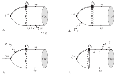
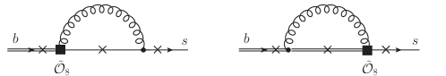
Figure 1: (top/middle) Diagrams $A_{1}$ to $A_{4}$ to which we refer to as spectator corrections (bottom) Non-spectator corrections. Crosses denote possible places for photon emission.

The diagrams are computed via the light-cone operator product expansion (LC-OPE), since the correlation function is believed to be dominated by light-like distances. Schematically this amounts to to a convolution between a perturbatively calculable hard scattering kernel $T_{H}$ and light-cone distribution amplitudes (DA) $\phi$:

$$\Pi(q^{2},p_{B}^{2})=\sum_{i}T^{(i)}_{H}(q^{2},p_{B}^{2};\mu_{F};u)\circ\phi^{(i)}(u,\mu_{F})\;.$$

The sum extends over increasing orders of twist, defined as the dimension of the operator minus its spin projection, and the variable $u$ stands for the momentum fraction of the strange quark in the light meson. We limit ourselves to leading twist-2.

3 Sum rules and anomalous thresholds

For the important steps of selecting cuts for the dispersion relation and Borel transformation we refer the reader to the main paper [1]. We shall quote here an intermediate expression,

$$\begin{split}\langle\gamma^{*}(q)V(p)|\tilde{O}_{8}|\bar{B}(p_{B})\rangle&=\\ \frac{1}{f_{B}m_{B}^{2}}\frac{1}{2\pi i}&\int_{\Gamma\backslash\Gamma_{\rm NP}}dse^{\frac{m_{B}^{2}-s}{M^{2}}}\Pi^{V}(q^{2},s)\;,\end{split}$$ (8)

that relates an on-shell matrix element to an integral over an off-shell correlation function. $\Gamma$ is a closed path on the physical Riemann sheet that does not contain any singularities such as poles and cuts. $\Gamma_{\rm NP}$ is of the same type except that it contains the pole of the matrix element. At this stage the relation is exact but admittedly rather cryptic. In sum rules the analytic structure of the correlation functions is usually such that the singularities are on the real line. In the case at hand though it happens that there is an anomalous threshold extending into the complex plane. Let us explain in more detail: after the reduction to scalar integrals the Passarino-Veltman function $C_{0}(s,u(s\!-\!m_{B}^{2}),\bar{u}m_{B}^{2}\!+\!uq^{2},0,m_{b}^{2},0)$ (where $s=p_{B}^{2}$) appears in the expression for $G_{\iota}^{(s)}(q^{2})$, c.f. Fig. 2. The fact that this function has an anomalous threshold extending into the lower half-plane, for $q^{2}>0$ and appropriate momentum fraction $u$, can be seen in various ways. First, using the explicit result valid on the real line we can show by uniqueness of analytic continuation from the real line that there must be singularities in the complex plane [1]. Second, by setting $m_{B}^{2}<0$ in the dispersion integral we see that its path is deformed into the lower complex plane by analytic continuation of $m_{B}^{2}$ to its physical value [1]. The analytic structure of this function is depicted in Fig. 2 for a simplified set of variables. Further to that, the work of Källén and Wightman [16] shows that anomalous thresholds are present in the corresponding triangle function of the full theory using a minimal number of axioms. This almost implies that the anomalous thresholds are present in the full theory: the loophole is that the reduction to a scalar object in the non-perturbative case is not as efficient as for the one-loop case; thus it could in principle be that the contributions cancel, however this is unlikely and in any case not relevant to our discussion. The important point is that the ${\rm Re}[s_{-}]$ and thus the rest the anomalous branch cut is well above the $m_{B}$-pole, and the anomalous cut is part of what is usually called the continuum contribution in sum rules. In the following paragraph we aim to discuss to what extent these anomalous thresholds are surprising and what their meaning is in the hope of clarifying to the reader some of our brief argumentation above.

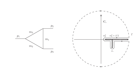
Figure 2: (left) Triangle graph corresponding to the $C_{0}(p_{1}^{2},p_{2}^{2},p_{3}^{2},m_{2}^{2},m_{3}^{2},m_{1}^{2})$ PV-function. The conventions are the same as in LoopTools [14] and Feyncalc [15]. (right) analytic structure of $C_{0}(s,s-\beta,\alpha,0,m_{b}^{2},0)$ in the $\mathbb{C}_{s}$-plane; more precisely this corresponds to the physical sheet. The leading Landau singularities of this triangle function are $s_{\pm}=m_{b}^{2}+\beta/2\pm\sqrt{(\beta/2)^{2}-\alpha m_{b}^{2}}$. As discussed in the text $s_{-}$ is on the physical sheet whereas $s_{+}$ is not.

The crucial point is that the correspondence between matrix elements and correlation functions is complicated when the number of legs increases. Let us begin by discussing the simplest case. For a two-point function of gauge invariant operators, a dispersion representation is in one-to-one correspondence with the insertion of a complete set of states as is explicit in the celebrated Källén-Lehmann representation [18] and derivations thereof. Thus the analytic structure in the complex plane of the four momentum invariant has a cut and poles on the real line starting from the lowest state in the spectrum. For correlation functions with three or more fields, there is no such direct relation. It seems preferable to think of the analytic structure (singularity structure) as a fundamental part of the correlation function rather than as the insertion of a complete set of states. For the dispersion relation, which is essentially an application of Cauchy’s integral theorem, it is immaterial whether the singularities are of the normal or anomalous type. Normal thresholds are related to unitarity, that is to say to the insertion of a complete set of states. Anomalous thresholds do not have such an interpretation. In fact, the anomalous threshold of the triangle graph in perturbation theory corresponds to the leading Landau singularity which in turn amounts to setting all the propagators on the mass shell. One out of the two solutions $s_{\pm}$ of the (leading) Landau equations turns out to be the end of the anomalous threshold (Fig. 2), whereas the other one is not on the physical sheet. We should add that determining which Riemann-sheet a complex singularity is on is generally a difficult problem.

4 Results

We refer the reader to reference [1] for some explicit analytic results. The results of $G_{\iota}^{(s)}(q^{2})$ and $G_{\iota}^{(ns)}(q^{2})$ are collected in appendices A and C of that reference. Amongst all the possible flavour transitions, only four are characteristically different depending on whether the initial meson is neutral or charged and whether it is of the beauty or charm type. Various subparts of this class, at $q^{2}=0$, are collected in Tab. 1. The ratio of $G_{1}^{(s)}$ to $T_{1}(0)$ can be understood as a radiative correction and is proportional to $\alpha_{s}(m_{b(c)})/(4\pi)$ times other factors of ${\cal O}(1)$. Further semi-quantitative insight can be gained by considering the heavy quark scaling of the matrix elements which is $m_{b}^{-3/2}$ except for diagrams $A_{1,2}$ which scale as $m_{b}^{-5/2}[\ln(m_{b})+{\cal O}(1)]$ as discussed in section 5. Projecting out the quark charges the respective ratios of $G_{1}^{D}(0)$ to $G_{1}^{B}(0)$ follow the ratio of heavy quark scaling and $\alpha_{s}(\sqrt{m_{c}\Lambda_{\rm had}})/\alpha_{s}(\sqrt{m_{b}\Lambda_{\rm had}})$ surprisingly well.

$$\begin{array}[]{ l | rr }{\rm type}&B^{-}\to\rho^{-}\gamma&\bar{B}^{0}\to\rho^{0}\gamma\\ \hline\cr G_{1}^{(s)}(0)\cdot 10^{2}&0.30-0.41i&0.23+0.21i\\ G_{1}^{(ns)}(0)\cdot 10^{2}&0.90+1.3i&0.90+1.3i\\ G_{1}(0)\cdot 10^{2}&1.2+0.89i&1.1+1.5i\\ \hline\cr\left|G_{1}^{(s)}/G_{1}^{(ns)}\right|(0)&32\%&20\%\\ \left|G_{1}^{(s)}/T_{1}\right|(0)&2\%&1\%\\ \left|G_{1}/T_{1}\right|(0)&6\%&7\%\\ \hline\cr\hline\cr{\rm type}&D^{+}\to\rho^{+}\gamma&D^{0}\to\rho^{0}\gamma\\ \hline\cr G_{1}^{(s)}(0)\cdot 10^{2}&-1.9+2.6i&-7.4-5.2i\\ G_{1}^{(ns)}(0)\cdot 10^{2}&-8.5-12i&-8.5-12i\\ G_{1}(0)\cdot 10^{2}&-11-9.4i&-16-17i\\ \hline\cr\left|G_{1}^{(s)}/G_{1}^{(ns)}\right|(0)&21\%&59\%\\ \left|G_{1}^{(s)}/T_{1}\right|(0)&5\%&13\%\\ \left|G_{1}/T_{1})\right|(0)&21\%&34\%\end{array}$$

Table 1: Comparison of various parts of the four characteristic types of $G_{\iota}$ matrix elements. For the short distance form factor $T_{1}(0)$ we use $T_{1}^{B}(0)=0.27$ [12] and $T^{D}_{1}(0)=0.7$ [8] as reference values. Recall $G_{1}(0)=G_{1}^{(s)}(0)+G_{1}^{(ns)}(0)$ and $G_{1}^{(s)}(0)=G_{1}^{(\perp)}(0)$ at our level of twist approximation.

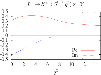
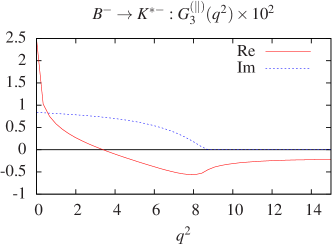
Figure 3: See caption of Fig. 4

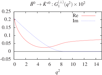
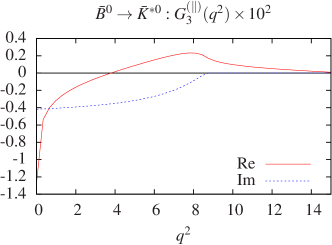
Figure 4: Plots of $G^{(\perp)}_{1}(q^{2})$ and $G_{3}^{(\parallel)}(q^{2})$ for charged (c.f. Fig. 3) and uncharged $B$ meson. These plots make it clear why one the $G_{\iota}(q^{2})$-functions are not referred to as form factors as they do not reveal a particular structure but parameterise a multitude of effects amongst which long distance contributions play a definite rôle. The results are valid in the region of $q^{2}$ above $1\,{\rm GeV}^{2}$, that is to say outside the resonance region and say $3\,{\rm GeV}^{2}$ below $m_{b}^{2}$.

We consider it worthwhile to quickly mention how the various projections of the DAs contribute to the matrix elements and how they are interrelated. At twist-2 there are seven contributions:

$$G_{i}^{(s)} = G_{i}^{(\perp)}(q^{2})+G_{i}^{(\parallel)}(q^{2})\;,$$

$$G_{T}^{(s)} = G_{T}^{(P)}(q^{2})\;,$$ (9)

It turns out that (4) can be fully reconstructed by knowing the three subparts $G_{1}^{(\perp)}(q^{2})$, $G_{3}^{(\parallel)}(q^{2})$ and $G_{T}^{(P)}(q^{2})$. Thus there are four relations: $G^{(\parallel)}_{1}(q^{2})=0$, $G^{(\parallel)}_{2}(q^{2})=0$, $G^{(\perp)}_{2}=(1-q^{2}/m_{B}^{2})G^{(\perp)}_{3}$ and $G^{(\perp)}_{2}=(1-q^{2}/m_{B}^{2})G^{(\perp)}_{1}$. The third relation assures a finite decay width in the limit $m_{V}^{2}\to 0$ (as employed here) [6]. The fourth relation is of the large energy effective theory (LEET)-type as found for form factors [13], whose origin is explained in appendix A of [DLZ] using the third relation and a generic ansatz. Furthermore, in the ultra-relativistic approximation $m_{V}^{2}\to 0$, the projections $G_{T}^{(P)}(q^{2})$ $G_{3}^{(\parallel)}(q^{2})$ are proportional to each other modulo a replacement of the corresponding DA. Thus the results can be understood qualitatively from the plots of $G_{1}^{(\perp)}$ and $G_{3}^{(\parallel)}$ c.f. Fig. 3,4 as the DA of $\phi^{\parallel}(u)$ and $\phi^{P}(u)$ hardly differ in practice. The uncertainties, which are added in quadrature, are estimated to be between $25\%$ and $35\%$ [1], for the $b$ and $c$-transitions respectively, depending on the hadronic input. It worthwhile to point out that the uncertainties are higher for the charm transitions because of the low scale for $\alpha_{s}$.

5 Comparison with QCD-factorisation

We shall summarise here a few points of the discussion in chapter 5 of [1] on comparing the contributions of diagrams $A_{1,2}$ of Fig. 1 in the QCDF and LCSR approaches. These diagrams form a well defined subset as they are isospin dependent. Parameterising $G_{1}(0)$ as

$$G_{1}(0)={\cal O}(m_{b}^{-5/2})\underbrace{\int_{0}^{1}\phi_{\perp}(u)x_{\perp}(u)}_{\equiv X_{\perp}}+{\cal O}(Q_{b})\;,$$

the QCDF [2] and LCSR [1] results read

$$x_{\perp}^{QCDF}(u) = \frac{1+\bar{u}}{3\bar{u}^{2}}\;,$$

$$x_{\perp}^{LCSR}(u) = \int_{m_{b}^{2}}^{s_{0}}ds\,e^{\frac{m_{B}^{2}-s}{M^{2}}}\rho(s,u)\;,$$ (10)

with $\bar{u}\equiv 1-u$ and

$$\rho(s,u)={\cal O}(m_{b}^{3})\left[\frac{\log\left(\frac{\bar{u}s(m_{b}^{2}+m_{B}^{2}-s)}{m_{B}^{2}(m_{b}^{2}-us)}\right)}{m_{B}^{2}-\bar{u}s}-\frac{s-m_{b}^{2}}{\bar{u}sm_{B}^{2}}\right]\;.$$

The endpoint divergence in QCDF arises as follows: assuming an endpoint behaviour $\phi_{\perp}(u)\stackrel{{\scriptstyle u\simeq 1}}{{\to}}6\bar{u}u$, which is true at every finite order in the Gegenbauer expansion, it is readily seen that $X_{\perp}^{QCDF}$ is logarithmically divergent (at the endpoint $u=1$). On a purely technical level this happens because two propagators behave as $1/\bar{u}m_{B}^{2}$ c.f. Fig. 5. In LCSR there is only one propagator with manifest $1/(\bar{u}m_{B}^{2})$-behaviour (c.f. Fig. 5) and there is no such term hidden in the loop as it would correspond to a power IR-divergence, and it is known that in four dimensions IR-singularities, whether they are soft or collinear, are at worst of logarithmic nature, e.g. [19]. Thus the worst behaviour that we can get is $x^{LCSR}_{\perp}\sim\ln\bar{u}/\bar{u}$ which is integrable, i.e. does not show an endpoint-divergence. Inspection or evaluation Eq. (5) gives an even milder behaviour with $x^{LCSR}_{\perp}\sim\ln\bar{u}$ for which we see no particular reason.

The comparison between QCDF and LCSR can be sharpened if the heavy quark scaling $m_{B}\to m_{b}+\bar{\Lambda}$, $s_{0}\to m_{b}^{2}+2m_{b}\omega_{0}$ and $M^{2}\to 2m_{b}\tau$, as suggested in [20], is applied:

$$X_{\perp}^{LCSR}\sim\ln(m_{b}/2\omega_{0})+{\cal O}(1)+{\cal O}\left(\frac{\Lambda_{\rm QCD}}{m_{b}}\right)\;.$$ (11)

The logarithmic term indicates that this expression is not expandable in inverse powers of the heavy quark mass. In fact, the expansion of the density around $m_{b}=\infty$ reveals that $\rho(s,u)\sim 1/(m_{b}^{n}\bar{u}^{n+1})$ in our results. Are the LCSR and the QCDF to be seen on an equal footing when the leading heavy quark scaling behaviour is considered? The answer must be no as the former has a sizeable imaginary part whereas the latter is real (at leading order in $\alpha_{s}$) [1]. This difference is due to the fact that LCSR contain additional contributions which are not present in the QCDF computation. An interpretation of the complex phase as a long distance phenomenon is given in the caption of Fig. 6.

In regards to the discussion above it is seems worthwhile to point out that even though QCDF and LCSR are both based on LC-expansions in terms of hard kernels and DAs they differ on a conceptual level. QCDF computes physical processes in a direct way and is in that sense very transparent. LCSR is of an indirect nature as correlation functions are computed in which the matrix element in question appears as a residue of a pole. The matrix element is then extracted by manipulating the sum rule (Borel transformation) and considering appropriate kinematical limits. In this sense LCSR is akin to lattice-QCD extraction of matrix elements.

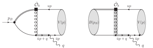
Figure 5: The shaded propagators scale like $1/(\bar{u}m_{B}^{2})$ in both figures. (left) Diagram used in LCSR. (right) Diagram used in QCDF. Thus $x_{\perp}^{QCDF}\sim 1/\bar{u}^{2}$ and $x_{\perp}^{LCSR}\sim\ln(\bar{u})/\bar{u}$ at worst, as explained in the text.

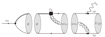
Figure 6: (left) Hadronic interpretation of the $3$-particle cut in in terms of a long-distance hadronic process. The state $(\bar{q}s)_{0^{\pm}}$ is any state, single or multiparticle, of spin zero with $\bar{q}$ and $s$ quantum numbers. The latter is a source for the strong (CP-even) phase that we obtain for the $G_{\iota}(q^{2})$-functions.

6 Conclusions

In this write up we have reported on the computation of matrix elements of heavy to light meson transitions induced by the ${\cal O}_{8}$ operator using LCSR. We focused on the appearance of a complex anomalous threshold and on comparing our results with those previously computed in QCDF. A characteristic feature of the results is a large strong phase reflecting the long distance physics contained in these matrix elements.

References

- [1] M. Dimou, J. Lyon and R. Zwicky, “Exclusive Chromomagnetism in heavy-to-light FCNCs,” Phys. Rev. D 87 (2013) 074008 arXiv:1212.2242 [hep-ph].
- [2] A. L. Kagan and M. Neubert, “Isospin breaking in gamma decays,” Phys. Lett. B 539 (2002) 227 [hep-ph/0110078].
- [3] T. Feldmann and J. Matias, “Forward backward and isospin asymmetry for decay in the standard model and in supersymmetry,” JHEP 0301 (2003) 074 [hep-ph/0212158].
- [4] Y. Y. Keum, M. Matsumori and A. I. Sanda, “CP asymmetry, branching ratios and isospin breaking effects of gamma with perturbative QCD approach,” Phys. Rev. D 72 (2005) 014013 [hep-ph/0406055].
- [5] P. Ball, G. W. Jones and R. Zwicky, “B —¿ V gamma beyond QCD factorisation,” Phys. Rev. D 75 (2007) 054004 [hep-ph/0612081].
- [6] J. Lyon and R. Zwicky, “Isospin asymmetries in and in and beyond the Standard Model,” arXiv:1305.4797 [hep-ph].
- [7] G. Isidori and J. Kamenik, “Shedding light on CP violation in the charm system via D to V gamma decays,” arXiv:1205.3164 [hep-ph].
- [8] J. Lyon and R. Zwicky, “Anomalously large and long-distance chirality from ,” arXiv:1210.6546 [hep-ph].
- [9] RAaij et al. [LHCb Collaboration], “Measurement of the isospin asymmetry in decays,” JHEP 1207 (2012) 133 [arXiv:1205.3422 [hep-ex]].
- [10] R. Aaij et al. [LHCb Collaboration], “Evidence for CP violation in time-integrated decay rates,” Phys. Rev. Lett. 108 (2012) 111602 [arXiv:1112.0938 [hep-ex]].
- [11] H. H. Asatrian, H. M. Asatrian, C. Greub and M. Walker, “Two loop virtual corrections to in the standard model,” Phys. Lett. B 507 (2001) 162 [hep-ph/0103087].
- [12] P. Ball and R. Zwicky, “ decay form factors from light-cone sum Phys. Rev. D 71 (2005) 014029 [arXiv:hep-ph/0412079].
- [13] J. Charles, A. Le Yaouanc, L. Oliver, O. Pene and J. C. Raynal, “Heavy to light form-factors in the heavy mass to large energy limit of QCD,” Phys. Rev. D 60 (1999) 014001 [hep-ph/9812358].
- [14] T. Hahn, M. Perez-Victoria, “Automatized one loop calculations in four-dimensions and D-dimensions,” Comput. Phys. Commun. 118 (1999) 153-165. [hep-ph/9807565].
- [15] R. Mertig, M. Bohm, A. Denner, “FEYNCALC: Computer algebraic calculation of Feynman amplitudes,” Comput. Phys. Commun. 64 (1991) 345-359.
- [16] G. Källén and A. S. Wightman: “The Analytic Properties of the Vacuum Expectation Value of a Product of Three Scalar Local Fields.” Mat. Fys. Skr. Dan. Vid. Selsk. 1, No. 6 (1958).
- [17] B.Anderson “Dispersion Relations for the Vertex Function from Local Commutativity.” CMP 25, 283–307 (1972).
-
[18]
G. Källén,
“On the definition of the Renormalization Constants in Quantum Electrodynamics,”
Helv. Phys. Acta 25 (1952) 417.
H. Lehmann, “On the Properties of propagation functions and renormalization contants of quantized fields,” Nuovo Cim. 11 (1954) 342. - [19] T. Muta, “Foundations of quantum chromodynamics. Second edition,” World Sci. Lect. Notes Phys. 57 (1998) 1.
- [20] V. L. Chernyak and I. R. Zhitnitsky, “B meson exclusive decays into baryons,” Nucl. Phys. B 345 (1990) 137.