Classical spin models Phase transitions: general studies Thermodynamics Order-disorder transformations

Dipolar needles in the microcanonical ensemble: evidence of spontaneous magnetization and ergodicity breaking

Abstract

We have studied needle shaped three-dimensional classical spin systems with purely dipolar interactions in the microcanonical ensemble, using both numerical simulations and analytical approximations. We have observed spontaneous magnetization for different finite cubic lattices. The transition from the paramagnetic to the ferromagnetic phase is shown to be first-order. For two lattice types we have observed magnetization flips in the phase transition region. In some cases, gaps in the accessible values of magnetization appear, a signature of the ergodicity breaking found for systems with long-range interactions. We analytically explain these effects by performing a nontrivial mapping of the model Hamiltonian onto a one-dimensional Ising model with competing antiferromagnetic nearest-neighbor and ferromagnetic mean-field interactions. These results hint at performing experiments on isolated dipolar needles in order to verify some of the exotic properties of systems with long-range interactions in the microcanonical ensemble.

Systems with long-range interactions, such as gravitational, Coulomb and magnetic systems, are of fundamental and practical interest because of their exotic statistical properties including ensemble inequivalence, negative specific heat, temperature jumps, ergodicity breaking, etc. [1] Recently, a number of mean-field type models have been developed which are very convenient for analytical understanding [2, 3]. However, up to now, the connection to real physical systems has not been seriously addressed (see, however, Refs. [4, 5, 6] for some progress in this direction). It is therefore crucial to propose experimentally testable effects.

Dipolar force is one of the best candidates for experimental and theoretical studies of long-range interactions [7]. For instance, experimental studies have been performed on layered spin structures [8]. For these systems, intralayer exchange is much larger than the interlayer one: hence, every layer can be identified as a single macroscopic spin. As a consequence, dipolar forces between layers are dominant and one can describe the system with an effective long-range one-dimensional model [5]. However, in order to perform a careful study of the statistical properties of such samples, one should simulate all the spins in each layer, which is computationally heavy.

Alternatively, one can consider purely dipolar systems known as dipolar ferromagnets [9, 10], where dipolar effects prevail over short-range exchange interactions. Long-range dipolar orientational order is also found theoretically for dipolar fluids confined in ellipsoidal geometries [11]. More recently, dipolar ferromagnetism has also been measured at ambient temperature in assemblies of closely-spaced cobalt nanoparticles [12].

It has been pointed out long ago [13] that body centered cubic (bcc) or face centered cubic (fcc) needle like samples should display spontaneous magnetization, while simple cubic (sc) lattices can be ordered only antiferromagnetically. On the other hand, it was later argued that dipolar systems cannot show nonzero magnetization in the thermodynamic limit [14], i.e. as a bulk property. All these theoretical studies were performed within the canonical ensemble, but we know that ensemble inequivalence is expected to be present also for dipolar systems [1]. This means that the phase diagram of dipolar systems can be different in the microcanonical ensemble: the location of phase transition points can vary, temperature jumps may appear and ergodicity may be broken [15, 3, 16]. It is therefore important to perform a study on samples with needle shape in the microcanonical ensemble. Experimentally, microcanonical ensemble measurements imply the realization of an isolated sample, or looking at time-scales that are fast with respect to the energy exchange rate with environment.

In this Letter, we study the microcanonical dynamics of dipolar needles via numerical simulations and analytical approximations. We want to check whether such systems can display spontaneous magnetization and study the nature of the paramagnetic/ferromagnetic phase transition.

Systems of classical spins with only dipolar interactions are described by the following Hamiltonian

$${\cal H}=\frac{\varepsilon}{2}\sum\limits_{i\neq j}\frac{a^{3}}{r_{ij}^{3}}\left(\vec{S}_{i}\cdot\vec{S}_{j}-3\frac{(\vec{S}_{i}\cdot\vec{r}_{ij})(\vec{S}_{j}\cdot\vec{r}_{ij})}{r_{ij}^{2}}\right),$$ (1)

where $|\vec{S}_{i}|=1$ is a unit vector located at the $i$-th lattice site, $\vec{r}_{ij}$ is the displacement vector between $i$-th and $j$-th site, $a$ stands for the lattice spacing and $\varepsilon=\mu_{0}\sigma^{2}/(4\pi a^{3})$ is an energy scale for dipolar interactions: for instance, in the case of cobalt nanoparticles with magnetic moment $\sigma\sim 2\cdot 10^{5}\mu_{B}$ and separation length $a\sim 20nm$ [12], this energy could be as large as $2500$K ($\mu_{0}$ is vacuum permeability and $\mu_{B}$ Bohr magneton).

The time evolution of the unit vector $\vec{S}_{i}$ is described by the torque equation

$$\frac{d{\vec{S}_{i}}}{dt}=\gamma{\vec{S}_{i}}\times{\vec{H}}_{i}\qquad\mbox{where}\qquad{\vec{H}}_{i}=-\frac{1}{\sigma}\frac{\partial{\cal H}}{\partial{\vec{S}_{i}}}.$$ (2)

Here, ${\vec{H}}_{i}$ is the local magnetic field acting on the spin attached to the $i$-th lattice site, $\gamma$ is the particle gyromagnetic ratio and, in numerical simulations, we measure time in units of $\mu/(\gamma\varepsilon)$.

In numerical experiments, we solve the torque equation for spins on sc, bcc and fcc lattices shown in Fig. 1. Initially, the spins are aligned along the main axis of the sample, as shown in the figure. In the course of time, we monitor the three components of the average magnetization $\vec{m}=(1/N)\sum_{i=1}^{N}\vec{S}_{i}$, where $N$ is the number of spins over which we perform an average.

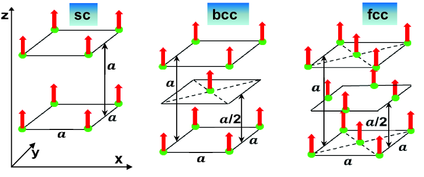
Figure 1: Cubic lattices considered in numerical simulations: simple cubic (sc), body centered (bcc) and face centered (fcc) cubic, respectively. The arrows indicate the initial direction of the spins while $a$ is the lattice spacing.

While for numerical simulations we directly use Hamiltonian (1) with the torque equation, our analytical approach is based on heuristic approximations by which we are able to map the main properties of Hamiltonian (1) onto those of the simple one-dimensional mean-field model studied in Ref. [3].

We consider samples elongated in the $z$-direction. This is the ordering direction of the spin system because the demagnetizing field is smaller along this axis. We follow the standard treatment in Refs. [17, 18] by dividing the sums in Hamiltonian (1) in two parts: The first part is the sum restricted only to a neighborhood of a site in the same layer (the reason this is done will be clear below), the second part is the sum over the remaining portion of the sample. We treat the latter sum, which takes into account the long-range character of the dipolar interaction, via a continuum approximation [18], which gives

$${\cal H}_{cont}=-\frac{\varepsilon a^{3}}{2\sigma^{2}}\int\left[\frac{4\pi}{3}\left(\vec{M}(\vec{r})\right)^{2}+\vec{H}^{m}(\vec{r})\vec{M}(\vec{r})\right]d^{3}r,$$ (3)

where the magnetization density $\vec{M}(\vec{r})$ is obtained by a local average over a macroscopic number of spins and $\vec{H}^{m}(\vec{r})$ is the demagnetizing field. In the case of ellipsoidal samples, there exists a uniform solution with demagnetizing field proportional to magnetization density $\vec{H}^{m}=-4\pi\hat{C}\vec{M}$, where

$$\vec{M}=\frac{\sigma}{V}\sum_{i=1}^{N}\vec{S}_{i}$$ (4)

and $\hat{C}$ stands for the demagnetization tensor. For simplicity, we neglect the transversal components of the spin vectors, only the longitudinal components $S_{i}^{z}$ are considered. As a further simplification, we assume that the longitudinal component takes only two values $S_{i}^{z}=\pm 1$, i.e. we reduce to Ising spins. After making such a crucial simplification, only the magnetization density along the $z$-axis is nonzero and we can easily perform the integral in formula (3), obtaining

$${\cal H}_{cont}=-\frac{\varepsilon a^{3}}{2Nv_{0}}\left[\frac{4\pi}{3}-4\pi C_{z}\right]\biggl{(}\sum\limits_{i=1}^{N}S^{z}_{i}\biggr{)}^{2},$$ (5)

where we have substituted $V=Nv_{0}$, $v_{0}$ being the volume per spin. It is important to point out that what we mean by volume is nontrivial in case of finite systems. We define the volume as the box that encloses the crystal so that the size of the box is obtained by matching total energies of the effective and discrete models. It turns out that in all lattices considered below this requires the box to be outstretching by a half a lattice constant from the spins at the boundary. This also has an effect on the definition of the aspect ratio.

As far as we consider only the $z$-components of the spins, it is easy to see that, for all considered lattices, in each layer transversal to the $z$-component of the sample, the coupling among the spins is antiferromagnetic. On the contrary, the coupling between neighboring spins in close transversal layers is ferromagnetic. This latter contribution is included in the ferromagnetic type coupling (5). Thus, incorporating nearest neighbor coupling terms and the terms appearing from the continuum approximation (5), we can reduce Hamiltonian (1) to the following effective Hamiltonian

$${\cal H}_{eff}=-\frac{K}{2}\sum\limits_{\langle i,i^{\prime}\rangle}\left(S^{z}_{i}S^{z}_{i^{\prime}}-1\right)-\frac{J}{2N}\biggl{(}\sum\limits_{i=1}^{N}S^{z}_{i}\biggr{)}^{2},$$ (6)

where the lattice dependent short-range coupling $K$ is heuristically estimated below, $\langle i,i^{\prime}\rangle$ means that the sum is restricted only to nearest-neighbors in the transversal layers and the ferromagnetic mean-field coupling constant $J$ is given by the following expression

$$J=\frac{4\pi\varepsilon a^{3}(1-3C_{z})}{3v_{0}},$$ (7)

while the demagnetizing coefficient $C_{z}$ is given by the following integral [18]

$$C_{z}=-\frac{1}{4\pi V}\int_{V}d^{3}r\int_{V}d^{3}r_{1}\frac{\partial^{2}}{\partial z^{2}}\left(\frac{1}{|\vec{r}-\vec{r}_{1}|}\right).$$ (8)

The demagnetizing coefficient $C_{z}$ is $1/3$ if the sample length $L$ coincides with the lattice spacing $a$, while it tends to zero if the aspect ratio $\xi=(L+a)/(2a)$ tends to infinity. In Fig. 2a, we plot the dependence of this coefficient on the aspect ratio, comparing the case of a parallelepiped with that of an ellipsoid, for which the exact expression is

$$C_{z}^{ell}=\frac{1-b^{2}}{2b^{3}}\left(\ln\frac{1+b}{1-b}-2b\right),$$ (9)

where $b=\sqrt{1-1/\xi^{2}}$. In all the estimates below, we use the demagnetizing coefficients of the parallelepiped, which gives a better quantitative agreement between analytical results derived from (6) and numerical simulations performed on (1).

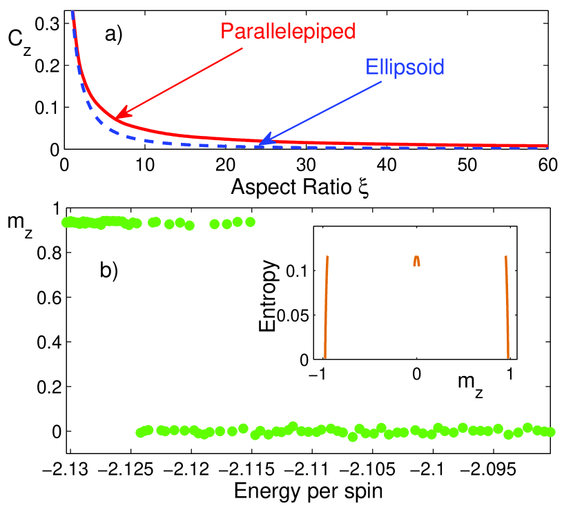
Figure 2: a) Demagnetizing coefficient $C_{z}$ computed numerically for a parallelepiped using formula (8) (solid line) versus the aspect ratio of the needle. We also plot the exact curve for an ellipsoid (dashed line), whose expression is given in formula (9). b) Final values of the $z$-component of the magnetization $m_{z}$ versus the energy per spin (in units of $\varepsilon$), obtained in numerical simulations of the sc lattice in Fig. 1. In the inset, we plot entropy versus magnetization of the effective Hamiltonian (6) at a typical energy in the range of the transition.

Let us remark that the second term in the effective Hamiltonian (6) contains the $z$-component of the average magnetization $m_{z}=(1/N)\sum_{i=1}^{N}S_{i}^{z}$, and its typical size can be varied by changing the aspect ratio $\xi$, i.e. the length $L$ of the sample.

We emphasize that the effective Hamiltonian (6) is the same as that in formula (1) of Ref. [3]. In the following, we will use results obtained for this Hamiltonian to discuss the phase diagram of model (1). Our approach consists in performing an estimate of the values of the couplings $K$ and $J$ based on features of the finite sample. In Ref. [3], it is proven that Hamiltonians of type (6) undergo a phase transition of the ferromagnetic type. This phase transition is of second order if both couplings $K$ and $J$ are positive. It becomes first order if the coupling $K$ is sufficiently negative, which favors locally the antiferromagnetic phase. The phase transition is present for values above $K/J=-0.5$, while for values below the system is always in the paramagnetic phase. Hence, what determines the presence of the phase transition in model (1) is the ratio $K/J$. This ratio can be estimated using the above expression of $J$ for particular choices of the lattice (e.g. those of Fig. 1) and by a rough estimate of the coupling constant $K$.

For simple cubic lattices (see Fig. 1) which have four spins in the transversal layer, the coupling constant $K=-2\varepsilon$. For $\xi\rightarrow\infty$, Eq. (8) leads to $J=4\pi\varepsilon/3$, since the volume per spin in a sc lattice is $v_{0}=a^{3}$. Thus, $K/J=-3/(2\pi)>-0.5$ and, therefore, we can expect the presence of a ferromagnetic phase.

In order to verify this prediction, we have performed numerical simulations of model (1), on a $2\times 2\times 50$ sc lattice, starting from a fully magnetized initial state, i.e. all spins pointing strictly along the $z$-axis. We then vary the energy of the initial state by adding random transversal components to the spins. We let the system relax towards a stationary state (this typically happens at times of the order $10^{4}$) and monitor the final value of $m_{z}$ for each value of the energy. We checked that the final state does not contain domains by looking at the spatial patterns of the individual spins. Collecting all these final values of the magnetization, we plot them as a function of energy per spin in Fig. 2b. We clearly observe a jump in magnetization from a positive value to zero and the presence of a coexistence region, where both a paramagnetic and a ferromagnetic phase are present, in full accordance with the predictions of the effective Hamiltonian (6) that the phase transition is first-order in the microcanonical ensemble. For symmetry reasons, we would have observed also the negative magnetization state if we had prepared the sample with the spins aligned opposite to the $z$-axis. The existence of this symmetry is confirmed by looking at the entropy of the effective Hamiltonian (6) (see Eq. (3) in [3]) as a function of $m_{z}$, shown in the inset of Fig. 2b. The gaps in the accessible values of magnetization are a signature of ergodicity breaking [3, 15, 16] . The first order phase transition takes place when the maxima of the entropy of the paramagnetic and ferromagnetic states are at the same height.

As we vary the size and the shape of the sample, the couplings $K$ and $J$ in Hamiltonian (1) change. We have then to check whether we are still in a region of parameters where the phase transition is present. It happens that for a sc lattice, an increase of the base size cancels the phase transition and the system always remains in the paramagnetic phase. Indeed for a wider base, each spin has four neighbors and thus the effective antiferromagnetic coupling constant $K=-4\varepsilon$, while the ferromagnetic mean-field constant remains $J=4\pi\varepsilon/3$ even for large aspect ratios. Therefore the ratio $K/J\approx-1$ does not allow for magnetized states to exist. This has been verified in numerical simulations which show that, even in the case of a $3\times 3$ base, there is no phase transition.

In order to verify whether other types of lattices can support phase transitions as suggested in [13], we have performed simulations for the bcc and fcc lattices shown in Fig. 1. We have shown that these lattices do have a phase transition if the aspect ratio is large enough, and therefore these dipolar samples display spontaneous magnetization.

For body centered cubic lattices, we have four spins in a layer and one spin in the neighboring layer. In the layer with four spins, the situation is exactly the same as that of the sc lattices, while in the layer with one spin there is no intralayer interaction. Thus, 4/5 of all spins can be treated as in sc lattices, while one of the five cannot have an antiferromagnetic coupling. These latter spins form a vertical chain, and their contribution to the Hamiltonian is a simple energy shift. Thus, the effective Hamiltonian for this lattice takes the form

$${\cal H}_{eff}^{bcc}=\frac{4}{5}{\cal H}_{eff}+\frac{1}{5}NE_{0}.$$ (10)

The antiferromagnetic coupling constant $K$ is unchanged. On the contrary, the mean-field ferromagnetic coupling constant $J$ changes since the average volume per spin is now $v_{0}=4a^{3}/5$, which implies that for large aspect ratios $J=5\pi\varepsilon/3$. As a consequence, $K/J\approx-0.4$ and, from what we know of Hamiltonian (6), we can therefore expect many different regimes, contrary to the case of sc lattices, where the ratio $K/J$ is close to $-0.5$.

In the following, we will need an estimate of the value of the energy shift $E_{0}$. Two ferromagnetic contributions appear in this quantity: the first one comes from the sum over all the sample while the second one derives from the sum over the neighboring spins along the vertical chain. For large aspect ratios, one has approximately $E_{0}=\left[-5\pi/3-4\right]\varepsilon/2$.

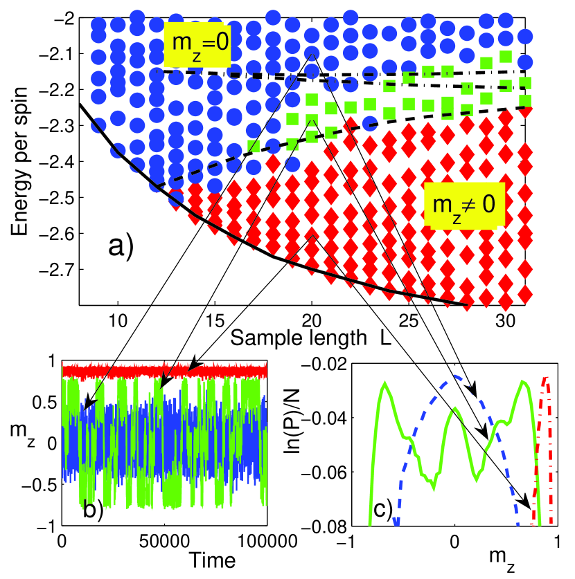
Figure 3: a) Phase diagram of Hamiltonian (1) for the bcc lattice in Fig. 1. Circles (blue), diamonds (red) and squares (green) represent paramagnetic, ferromagnetic and flipping states, respectively. The solid line is the minimal energy computed using Hamiltonian (10), the dashed one is the phase transition line and the dash-dotted lines are the bounds of the region with magnetization flips, again computed with the same effective Hamiltonian. b) Time evolution of the magnetization in different energy regions as shown by the arrows: $L=20$ with an energy per spin $-2.6$ (ferromagnetic ), $-2.3$ (flips) and $-2.1$ (paramagnetic); in all graphs energy is scaled in units of $\varepsilon$. c) Entropy per spin for the three phases in panel b).

We have performed numerical simulations for the bcc lattice of the full dipolar Hamiltonian (1). We have first concentrated our attention on detecting the presence of a phase transition. As control parameters, we use the energy per spin and the length $L$ of the sample. In Fig. 3a, we plot with circles the paramagnetic states and with diamonds the ferromagnetic ones. The minimal energy for each sample length is calculable from Hamiltonian (10) and is shown by the solid line in Fig. 3a: the agreement with numerical simulations of Hamiltonian (1) is also very good.

The effective Hamiltonian (10) predicts the location of the phase transition energies for each value of $K/J>-0.5$ (dashed line in Fig. 3a). The calculation can be performed by looking at entropy versus magnetization: near the phase transition point this curve is characterized by three disconnected humps, one at zero magnetization and two others at negative and positive magnetizations. On increasing energy from low values, the entropy at nonzero magnetization increases, while the zero magnetization entropy decreases: they become equal at the phase transition point. One should emphasize that, both below and above the phase transition energy, the entropy/magnetization curve is disconnected, showing ergodicity breaking. Only after a further increase of energy, the curve becomes connected with still three humps: this energy regime corresponds to the region where magnetization $m_{z}$ flips among positive, negative and zero values. This region is delimited by the dash-dotted lines in Fig. 3a.

Numerical simulations confirm the presence of a region of magnetization flips as shown in Fig. 3b, but not precisely at the same location in the parameter space that we predict. In Fig. 3c, we plot for three different energies the entropy per spin $s=(\ln P(m_{z}))/N$ where $P(m_{z})$ is obtained from the histogram of the magnetization. The first energy is in the paramagnetic phase and the entropy correctly shows a single hump centered around zero magnetization. A second energy is in the region of flips and the entropy shows three peaks, one centered at zero and two symmetric ones centered at positive and negative values of the magnetization. Finally, a third energy in the ferromagnetic phase shows a single peak at a positive value of the magnetization. It is likely that for this energy value we are in presence of magnetization gaps, i.e. ergodicity breaking, since a symmetric value of magnetization should be present at this energy, but cannot be reached using microcanonical dynamics. Like for sc lattices, we have checked whether the phase transition persists if one increases the size of the base of the bcc lattice. With four spins in the transversal layers, we get $K/J=-3/(2\pi)>-0.5$, which predicts that magnetized states can be realized in the bcc lattice even for large bases and for large aspect ratios. This is confirmed in numerical simulations.

Finally, let us switch to face centered cubic lattices. In the simplest realization of this lattice, there are four and five spins in subsequent transversal layers (see Fig. 1). Numerical simulations show the same phenomenology as the one of bcc lattices, for the smaller lengths. However, by looking at the effective Hamiltonian for this lattice, we can predict that, like for the sc lattice, magnetization does not persist for larger bases. Indeed, each spin interacts with four neighbors inside a transversal layer and, thus, the antiferromagnetic coupling constant $K=-8\sqrt{2}\varepsilon$. The volume per spin is $v_{0}=a^{3}/4$ and therefore $J=16\pi\varepsilon/3$ for large bases and large aspect ratios. Consequently, $K/J=-3/(\sqrt{2}\pi)<-0.5$, which excludes the presence of spontaneous magnetization.

As the length of the sample increases the system becomes more and more one-dimensional. One might therefore doubt about the existence of spontaneous magnetization for large aspect ratios, because dipolar force is short-range in one dimension. However, it is well known that, while one dimensional systems do not spontaneously magnetize, they nevertheless have a diverging correlation length at small temperatures $T$, $\ell=-a/\ln(\tanh(g/T))$, where $g$ is the short-range coupling constant. We would like to give an estimate of this correlation length to compare it with the sample lengths that we use. First of all, one can get an estimate of the temperature by treating canonically the single spin in interaction with the thermal bath of all other spins. In the mean-field approximation [19], $m_{z}=\tanh\left[\mu H/T\right]$ where $H=(K+J)m_{z}/\mu$ is assumed to be constant over the whole lattice. In our simulations for bcc lattices, the minimal magnetization for which the ferromagnetic state survives is in the range $m_{z}\simeq 0.65$. Using the mean-field formula above, we get the approximate value of the temperature of the system: $T\simeq 2\varepsilon$. The corresponding short-range coupling constant is $g=(K+J)/2\approx\varepsilon$, from which we get the value of the correlation length $\ell\approx a$. This value is much smaller than the typical length of the sample, and then we can conclude that the magnetization that we observe is not of short-range origin.

In conclusion, we have shown clear evidences of the presence of spontaneous magnetization in finite needle-like samples, within the microcanonical ensemble. We believe that the origin of this effect is in the long-range character of Hamiltonian (1), which we were able to map onto an effective one-dimensional Ising model with competing antiferromagnetic short-range and ferromagnetic mean-field couplings. The presence of jumps in magnetization as energy is varied, the coexistence of paramagnetic and ferromagnetic phases in some energy ranges, and the appearance of flips of magnetization are all indications that the phase transition we observe is of the first-order. We have simulated three different kinds of cubic lattices and all of them show spontaneous magnetization in some parameter ranges. Flips are found only for bcc and fcc lattices.

Magnetization flips which have features of telegraph noise have been observed experimentally for short-range ferromagnets [20]. Since rare-earth compounds  [9, 10] and cobalt nanoparticle assemblies [12] are dominated by long-range dipolar interactions, it could be extremely interesting to check experimentally the presence of magnetization flips in isolated purely dipolar samples.

Our numerical simulations also show that, in the ferromagnetic phase, gaps in the accessible values of magnetization appear. This is an indication of ergodicity breaking [3, 15, 16], one of the exotic properties of systems with long-range interactions [1] that could also be checked in experiments performed in microcanonical conditions.

- [1] A. Campa, T. Dauxois, S. Ruffo, Physics Reports 480, 57 (2009).
- [2] J. Barré, D. Mukamel, S. Ruffo, Phys. Rev. Lett. 87, 030601 (2001).
- [3] D. Mukamel, S. Ruffo, N. Schreiber, Phys. Rev. Lett. 95, 240604 (2005).
- [4] M. Chalony, J. Barré, B. Marcos, A. Olivetti, D. Wilkowski, Phys. Rev. A 87, 013401 (2013).
- [5] A. Campa, R. Khomeriki, D. Mukamel, S. Ruffo, Phys. Rev. B 76, 064415 (2007).
- [6] R. Bachelard, T. Manos, P. de Buyl, F. Staniscia, F.S. Cataliotti, G. De Ninno, D. Fanelli, N. Piovella, J. Stat. Mech.:Theory and Experiment P06009 (2010).
- [7] D. Mukamel, in Long-Range Interacting Systems, T. Dauxois, S. Ruffo, L. Cugliandolo (Eds.), Oxford University Press, Ch. 1, p. 33 (2009); S.T. Bramwell, ibid, Ch. 17, p. 549.
- [8] M. Sato, A. J. Sievers, Nature 432, 486 (2004).
- [9] P. Beauvillain, J.-P. Renard, I. Laursen, P.J. Walker, Phys. Rev. B 18, 3360 (1978); A. Biltmo, P. Henelius, Europhys. Lett. 87, 27007 (2009).
- [10] M.R. Roser, L.R. Corruccini, Phys. Rev. Lett. 65, 1064 (1990).
- [11] B. Groh, S. Dietrich, Phys. Rev. Lett. 72, 2422 (1994);ibid 74, 2617 (1995); H. Zhang and M. Widom, Phys. Rev. Lett. 74, 2616 (1994).
- [12] M. Varon et al., Sci. Rep. 3, 1234 (2013).
- [13] J. M. Luttinger, L. Tisza, Phys. Rev. 70, 954 (1946); 72, 257 (1947).
- [14] R. B. Griffiths, Phys. Rev. 176, 655 (1968).
- [15] F. Borgonovi, G. L. Celardo, M. Maianti, E. Pedersoli, J. Stat. Phys. 116, 516 (2004).
- [16] F. Bouchet, T. Dauxois, D. Mukamel, S. Ruffo, Physical Review E 77, 011125 (2008 )
- [17] L.D. Landau, E.M. Lifshitz, Course of Theoretical Physics, Vol. 8: Electrodynamics of Continuous Media, London, Pergamon (1960).
- [18] A.I. Akhiezer, V.G. Baryakhtar, S.V. Peletminskij, Spin Waves, Amsterdam, North Holland (1968).
- [19] A. Abragam, M. Goldman, Nuclear Magnetism: Order and Disorder, Clarendon Press, Oxford (1982).
- [20] W. Wernsdorfer, E.B. Orozco, K. Hasselbach, A. Benoit, B. Barbara, N. Demoncy, A. Loiseau, H. Pascard, D. Mailly, Phys. Rev. Lett. 78, 1791 (1997).