MAGNETIC SUSCEPTIBILITY AND LANDAU DIAMAGNETISM OF QUANTUM COLLISIONAL DEGENERATE PLASMAS

A. V. Latyshev and A. A. Yushkanov

Faculty of Physics and Mathematics,
Moscow State Regional University, 105005,
Moscow, Radio str., 10–A

Abstract

With the use of correct expression of the electric conductivity of quantum collisional degenerate plasmas the kinetic description of a magnetic susceptibility is obtained and the formula for calculation of Landau diamagnetism is deduced.

Key words: degenerate collisional plasma, magnetic susceptibility, transverse electric conductivity, Landau diamagnetism.

PACS numbers: 52.25.Dg Plasma kinetic equations, 52.25.-b Plasma properties, 05.30 Fk Fermion systems and electron gas

Introduction

Magnetisation of electron gas in a weak magnetic fields compounds of two independent parts (see, for example, [1]): from the paramagnetic magnetisation connected with own (spin) magnetic momentum of electrons (Pauli’s paramagnetism, W. Pauli, 1927) and from the diamagnetic magnetisation connected with quantization of orbital movement of electrons in a magnetic field (Landau diamagnetism, L. D. Landau, 1930).

Landau diamagnetism was considered till now for a gas of the free electrons. It has been thus shown, that together with original approach developed by Landau, expression for diamagnetism of electron gas can be obtained on the basis of the kinetic approach [2].

The kinetic method gives opportunity to calculate the transverse dielectric permeability. On the basis of this quantity its possible to obtain the value of the diamagnetic response.

However such calculations till now were carried out only for collisionalless case. The matter is that correct expression for the transverse dielectric permeability of quantum plasma existed till now only for gas of the free electrons. Expression known till now for the transverse dielectric permeability in a collisional case gave incorrect transition to the classical case [3]. So this expression were accordingly incorrect.

Central result from [4] connects the mean orbital magnetic moment, a thermodynamic property, with the electrical resistivity, which characterizes transport properties of material. In this work was discussed the important problem of dissipation (collisions) influence on Landau diamagnetism. The analysis of this problem is given with use of exact expression of transverse conductivity of quantum plasma.

In work [5] is shown that a classical system of charged particles moving on a finite but unbounded surface (of a sphere) has a nonzero orbital diamagnetic moment which can be large. Here is considered a non-degenerate system with the degeneracy temperarure much smaller than the room temperature, as in the case of a doped high-mobility semiconductor.

In work [6] for the first time the expression for the quantum transverse dielectric permeability of collisional degenerate plasma has been derived. The obtained in [6] expression for transverse dielectric permeability satisfies to the necessary requirements of compatibility.

In the present work for the first time with use of correct expression for the transverse conductivity [6] the kinetic description of a magnetic susceptibility of quantum collisional degenerate plasmas is given. The formula for calculation of Landau diamagnetism for degenerate collisional plasmas is deduced.

2. Magnetic susceptibility of quantum degenerate plasmas

Magnetization vector $\mathbf{M}$ of electron plasma is connected with current density $\mathbf{j}$ by the following expression [7]

$${\bf j}=c\,{\rm rot}\,\mathbf{M},$$

where $c$ is the light velocity.

Magnetization vector $\mathbf{M}$ and a magnetic field strength $\mathbf{H}=\rm rot\mathbf{A}$ are connected by the expression

$${\bf M}=\chi\,{\bf H}=\chi\,{\rm rot}\,{\bf A},$$

where $\chi$ is the magnetic susceptibility, $\mathbf{A}$ is the vector potential.

From these two equalities for current density we have

$$\mathbf{j}={c}\,{\rm rot}\,\mathbf{M}=c\,\chi{\rm rot}\,\big{(}{\rm rot}\,\mathbf{A}\big{)}=c\,\chi\,\big{[}{\bf\nabla}({\bf\nabla}\cdot{\bf A})-{\mathbf{\triangle}}\mathbf{A}\big{]}.$$

Here $\Delta$ is the Laplace operator.

Let the scalar potential is equal to zero. Vector potential we take orthogonal to the direction of a wave vector $\mathbf{q}$ ($\mathbf{q}\mathbf{A}=0$) in the form of a harmonic wave

$$\mathbf{A}(\mathbf{r},t)=\mathbf{A}_{0}e^{i(\mathbf{q}\mathbf{r}-\omega t)}.$$

Such vector field is solenoidal

$$\mathop{\rm div}\mathbf{A}=\nabla\mathbf{A}=0.$$

Hence, for current density we receive equality

$${\bf j}=-c\,\chi\Delta\mathbf{A}=c\,\chi\,q^{2}\mathbf{A}.$$

On the other hand, connection of electric field $\mathbf{E}$ and vector potential $\mathbf{A}$ is as follows

$$\mathbf{E}=-\dfrac{1}{c}\dfrac{\partial\mathbf{A}}{\partial t}=\dfrac{i\omega}{c}\mathbf{A}.$$

It is leads to the relation

$$\mathbf{j}=\sigma_{tr}\mathbf{E}=\sigma_{tr}\dfrac{i\omega}{c}\mathbf{A},$$

where $\sigma_{tr}$ is the transverse electric conductivity.

For our case from (1.1) and (1.2) we obtain following expression for the magnetic susceptibility

$$\chi=\dfrac{i\omega}{c^{2}q^{2}}\sigma_{tr}.$$

Expression of transversal conductivity of degenerate collisional plasmas it is defined by the general formula [6]:

$$\sigma_{tr}({\bf q},\omega,\nu)=\sigma_{0}\dfrac{i\nu}{\omega}\Big{(}1+\dfrac{\omega J({\bf q},\omega,\nu)+i\nu J({\bf q},0,0)}{\omega+i\nu}\Big{)},$$

where $\sigma_{0}$ is the static conductivity, $\sigma_{0}={e^{2}N}/{m\nu}$, $N$ is the concentration (number density) of plasmas particles, $e$ and $m$ is the electron charge and mass, $\nu$ is the effective collisional frequency of plasmas particles,

$$J({\bf q},0,0)=\dfrac{\hbar^{2}}{8\pi^{3}mN}\int\dfrac{f_{\bf k}-f_{\bf k-q}}{\mathcal{E}_{\bf k}-\mathcal{E}_{\bf k-q}}{\bf k}_{\perp}^{2}d^{3}k,$$

$$J({\bf q},\omega,\nu)=\dfrac{\hbar^{2}}{8\pi^{3}mN}\int\dfrac{f_{\bf k}-f_{\bf k-q}}{\mathcal{E}_{\bf k}-\mathcal{E}_{\bf k-q}-\hbar(\omega+i\nu)}{\bf k}_{\perp}^{2}d^{3}k,$$

$$f_{\bf k}=\Theta(\mathcal{E}_{\bf k}-\mathcal{E}_{F}),$$

$\Theta(x)$ is the function of Heaviside, $\mathcal{E}_{\bf k}={\hbar^{2}{\bf k}^{2}}/{2m}$ is the electron energy, $\mathcal{E}_{F}={mv_{F}^{2}}/{2}$ is the electron energy on Fermi surface, $v_{F}$ is the electron velocity on Fermi surface, which is considered spherical, $\hbar$ is the Planck’s constant,

$$\Theta(x)=\left\{\begin{array}[]{c}1,\qquad x>0,\\ 0,\qquad x<0,\end{array}\right.$$

$${\bf k}_{\perp}^{2}={\bf k}^{2}-\Big{(}\dfrac{{\bf kq}}{q}\Big{)}^{2}.$$

According to (1.1) and (1.2) magnetic susceptibility of the quantum collisional degenerate plasmas it is equal

$$\chi({\bf q},\omega,\nu)=-\dfrac{e^{2}N}{mc^{2}q^{2}}\Big{(}1+\dfrac{\omega J({\bf q},\omega,\nu)+i\nu J({\bf q},0,0)}{\omega+i\nu}\Big{)}.$$

From the formula (1.3) it is visible, that at $\omega=0$ frequency of collisions plasma particles $\nu$ drops out of the formula (1.3). Hence, the magnetic susceptibility in a static limit does not depend from frequencies of collisions of plasma and the following form also has:

$$\chi({\bf q},0,\nu)=-\dfrac{e^{2}N}{mc^{2}q^{2}}\Big{[}1+\dfrac{\hbar^{2}}{8\pi^{3}mN}\int\dfrac{f_{\bf k}-f_{\bf k-q}}{\mathcal{E}_{\bf k}-\mathcal{E}_{\bf k-q}}{\bf k}_{\perp}^{2}d^{3}k\Big{]}.$$

From expression (1.3) it is visible, that a magnetic susceptibility in collisionless quantum degenerate plasma is equal:

$$\chi({\bf q},\omega,0)=-\dfrac{e^{2}N}{mc^{2}q^{2}}\Big{[}1+\dfrac{\hbar^{2}}{8\pi^{3}mN}\int\dfrac{f_{\bf k}-f_{\bf k-q}}{\mathcal{E}_{\bf k}-\mathcal{E}_{\bf k-q}-\hbar\omega}{\bf k}_{\perp}^{2}d^{3}k\Big{]}.$$

At $\omega\to 0$ the formula (1.5) passes in the formula (1.4).

Let’s deduce the formula for calculation of a magnetic susceptibility of quantum collisional degenerate plasmas.

After obvious linear replacement of variables the formula for integral $J({\bf q},\omega,\nu)$ will be transformed to the form

$$J=\dfrac{\hbar^{2}}{8\pi^{3}mN}\int\dfrac{(\mathcal{E}_{\bf k+q}+\mathcal{E}_{\bf k-q}-2\mathcal{E}_{\bf k})f_{\bf k}{\bf k}_{\perp}^{2}d^{3}k}{[\mathcal{E}_{\bf k}-\mathcal{E}_{\bf k-q}-\hbar(\omega+i\nu)][\mathcal{E}_{\bf k+q}-\mathcal{E}_{\bf k}-\hbar(\omega+i\nu)]}.$$

Let’s enter dimensionless variables

$$z=\dfrac{\omega+i\nu}{k_{F}v_{F}}=x+iy,\quad x=\dfrac{\omega}{k_{F}v_{F}},\quad y=\dfrac{\nu}{k_{F}v_{F}},\quad Q=\dfrac{q}{k_{F}}.$$

Then

$$\mathcal{E}_{\bf k}-\mathcal{E}_{\bf k-q}-\hbar(\omega+i\nu)=2\mathcal{E}_{F}Q\Big{(}K_{x}-\dfrac{z}{Q}-\dfrac{Q}{2}\Big{)},$$

$$\mathcal{E}_{\bf k+q}-\mathcal{E}_{\bf k}-\hbar(\omega+i\nu)=2\mathcal{E}_{F}Q\Big{(}K_{x}-\dfrac{z}{Q}+\dfrac{Q}{2}\Big{)},$$

$$\mathcal{E}_{\bf k+q}+\mathcal{E}_{\bf k-q}-2\mathcal{E}_{\bf k}=2\mathcal{E}_{F}Q^{2}.$$

Considering, that for degenerate plasmas $k_{F}^{3}=3\pi^{2}N$, on the basis (1.6) it is received

$$J(Q,z)=\dfrac{3}{8\pi}\int\dfrac{f_{\bf K}{\bf K}_{\perp}^{2}d^{3}K}{(K_{x}-z/Q)^{2}-(Q/2)^{2}},$$

where

$$f_{\bf K}=\Theta(1-{\bf K}^{2}),\qquad{\bf K}_{\perp}^{2}=K_{y}^{2}+K_{z}^{2}.$$

Now the formula (1.3) for a magnetic susceptibility can be written down in the form

$$\chi(Q,x,y)=-\dfrac{e^{2}v_{F}}{3\pi^{2}\hbar c^{2}Q^{2}}\Big{(}1+\dfrac{xJ(Q,z)+iyJ(Q,0)}{x+iy}\Big{)}.$$

Here according to (1.7)

$$J(Q,z)=\dfrac{3}{16}\int\limits_{-1}^{1}\dfrac{(1-\tau^{2})^{2}d\tau}{(\tau-z/Q)^{2}-(Q/2)^{2}}=-\dfrac{5}{8}+\dfrac{3z^{2}}{4Q^{2}}+\dfrac{3Q^{2}}{32}+$$

$$+\dfrac{3}{16Q}\Big{[}\Big{(}1-\dfrac{z^{2}}{Q^{2}}\Big{)}^{2}+\dfrac{Q^{4}}{16}-\dfrac{Q^{2}}{2}+\dfrac{3z^{2}}{2}\Big{]}\ln\dfrac{(1-Q/2)^{2}-(z/Q)^{2}}{(1+Q/2)^{2}-(z/Q)^{2}}-$$

$$-\dfrac{3zQ}{32}\Big{[}1+\dfrac{4}{Q^{2}}\Big{(}1-\dfrac{z^{2}}{Q^{2}}\Big{)}\Big{]}\ln\dfrac{(1-z/Q)^{2}-(Q/2)^{2}}{(1+z/Q)^{2}-(Q/2)^{2}},$$

$$J(Q,0)=-\dfrac{5}{8}+\dfrac{3Q^{2}}{32}+\dfrac{3(4-Q^{2})^{2}}{256Q}\ln\Big{(}\dfrac{2-Q}{2+Q}\Big{)}^{2}.$$

2. Landau diamagnetism of quantum degenerate collisionless plasmas

Landau diamagnetism in collisionless plasma is usually defined as a magnetic susceptibility in a static limit for a homogeneous external magnetic field. Thus the diamagnetism value can be found by means of (1.1) through two non-commutative limits

$$\chi_{L}=\lim\limits_{q\to 0}\Big{[}\lim\limits_{\omega\to 0}\chi(q,\omega,\nu=0)\Big{]}.$$

Into collisionless plasma this expression (2.1) should lead to the known formula of Landau’s diamagnetism

$$\chi_{L}=-\dfrac{1}{3}\left(\dfrac{e\hbar}{2mc}\right)^{2}\dfrac{p_{F}m}{\pi^{2}\hbar^{3}}=-\dfrac{e^{2}v_{F}}{12\pi^{2}\hbar c^{2}}.$$

Let’s deduce the formula of Landau’s diamagnetism (2.2) by means of expression (1.8). At $z=+iy=0$ from the formula (1.8) for magnetic susceptibility of the quantum collisionless degenerate plasmas we receive the following expression

$$\chi(Q)=-\dfrac{e^{2}v_{F}}{3\pi^{2}\hbar c^{2}Q^{2}}\Big{[}1+\dfrac{3}{8\pi}\int\dfrac{f_{\bf K}{\bf K}_{\perp}^{2}d^{3}K}{K_{x}^{2}-(Q/2)^{2}}\Big{]}=$$

$$=-\dfrac{e^{2}v_{F}}{3\pi^{2}\hbar c^{2}Q^{2}}\Big{[}1+\dfrac{3}{16}\int\limits_{-1}^{1}\dfrac{(1-\tau^{2})^{2}d\tau}{\tau^{2}-(Q/2)^{2}}\Big{]},$$

or, in explicit form

$$\chi(Q)=-\dfrac{e^{2}N}{mc^{2}k_{F}^{2}Q^{2}}\Big{[}\dfrac{3}{8}+\dfrac{3}{32}Q^{2}+\dfrac{3(Q^{2}-4)^{2}}{128Q}\ln\Big{|}\dfrac{2-Q}{2+Q}\Big{|}\Big{]}.$$

Noticing, that at small $Q$

$$\dfrac{1}{Q}\ln\dfrac{1-Q/2}{1+Q/2}=-1-\dfrac{Q^{2}}{12}-\cdots,$$

on the basis of (2.3) we found the known expression for diamagnetism of Landau for degenerate electronic gas

$$\chi_{L}=\lim\limits_{Q\to 0}\chi(Q)=-\dfrac{e^{2}k_{F}}{12\pi^{2}mc^{2}}=-\dfrac{e^{2}v_{F}}{12\pi^{2}c^{2}\hbar}.$$

Рис. 1: Diamagnetic susceptibility for the case $\omega=0$ into collisionless plasmas ($\nu=0$).

Having divided (2.3) on (2.4), we receive (see fig. 1) the relative magnetic susceptibility for quantum collisionless plasmas in static limit

$$\dfrac{\chi(Q)}{\chi_{L}}=\dfrac{4}{Q^{2}}\Big{[}\dfrac{3}{8}+\dfrac{3}{32}Q^{2}+\dfrac{3(Q^{2}-4)^{2}}{128Q}\ln\Big{|}\dfrac{2-Q}{2+Q}\Big{|}\Big{]}.$$

3. The analysis of results

Let’s present the formula (1.8) in the form

$$\dfrac{\chi(Q,z)}{\chi_{L}}=\dfrac{4}{Q^{2}}\Big{(}1+\dfrac{xJ(Q,z)+iyJ(Q,0)}{x+iy}\Big{)}.$$

For graphic research of a magnetic susceptibility we will be to use the formula (3.1).

From fig. 1 it is obvious, that in quantum collisionless plasma ($\nu=0$) in a static limit ($\omega=0$) the magnetic susceptibility is function of wave number monotonously decreasing to zero.

On fig. 2 and 3 the dependence of a magnetic susceptibility of collisionless plasmas as function of wave number (fig. 2) or function of dimensionless frequency of oscillations of an electromagnetic field $x$ (fig. 3) is presented.

From fig. 2 it is clear, that the magnetic susceptibility is monotonously decreasing function of wave number at all values of frequency of oscillations of electromagnetic field. Thus for all $x<1$ ($\omega<\omega_{p}$) values of a magnetic susceptibility that more than the quantity of frequency of oscillations of the electromagnetic field is mores.

From fig. 3 it is clear, that a magnetic susceptibility as function of frequencies of oscillations of a field has the maximum near to frequency $\omega=Q\omega_{p}$ and with growth $Q$ moves to the right.

On fig. 4 and 5 the dependence of real (fig. 4) and imaginary (fig. 5) parts of the magnetic susceptibility from the dimensionless frequency of oscillations of the field in the case $Q=0.5$ are presented.

From fig. 4 it is clear, that the real part has a maximum, which is

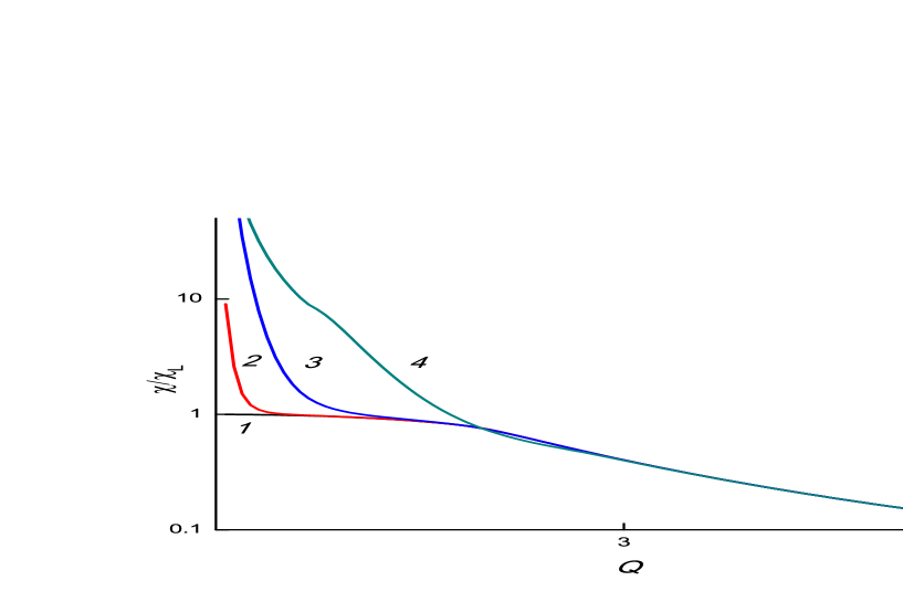
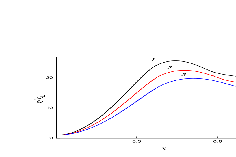
Рис. 2: Diamagnetic susceptibility of collisionless plasmas, curves $1$,$2$,$3$ and $4$ correspond to paramater quantities $x=0,0.01,0.1$ and $x=1$.

Рис. 3: Diamagnetic susceptibility of collisionless plasmas, curves $1$, $2$, $3$ correspond to paramater quantities $Q=0.45,0.50,0.55$.

displaced to the right with growth of frequency of collisions of plasmas.

Independently of the frequency of collisions of plasmas particles with growth of frequency of oscillations of electromagnetic field quantity of the real part of the magnetic susceptibility leaves from above on the asymptotic

$$\lim\limits_{x\to 0}\mathop{\rm Re}\Big{(}\dfrac{\chi(Q,x,y)}{\chi_{L}}\Big{)}=\dfrac{4}{Q^{2}}.$$

Not resulting necessary graphics we will inform, that with reduction quantity of wave number the maximum of magnetic susceptibility moves to the left and becomes sharp at small values of frequency collisions of plasmas particles. With growth of frequency of collisions the maximum starts to smooth out and vanishes.

From fig. 5 it is obvious, that the imaginary part of magnetic susceptibility as function of dimensionless frequency of oscillations of electromagnetic field has a minimum. This minimum moves to the left with growth collisions frequency of plasmas particles. With the growth of the dimensionless frequencies of oscillations of electromagnetic field an imaginary part of the magnetic susceptibilities leaves from below on the asimptotyc $\mathop{\rm Im\,}(\chi/\chi_{L})=0$. We will notice, that a minimum of an imaginary part not vanishes with growth as frequencies of collisions of particles of plasma, and of dimensionless wave number.

Let’s notice, that the frequency of collisions of plasma particles there is less, the more values of the real and imaginary parts magnetic susceptibilities turn out.

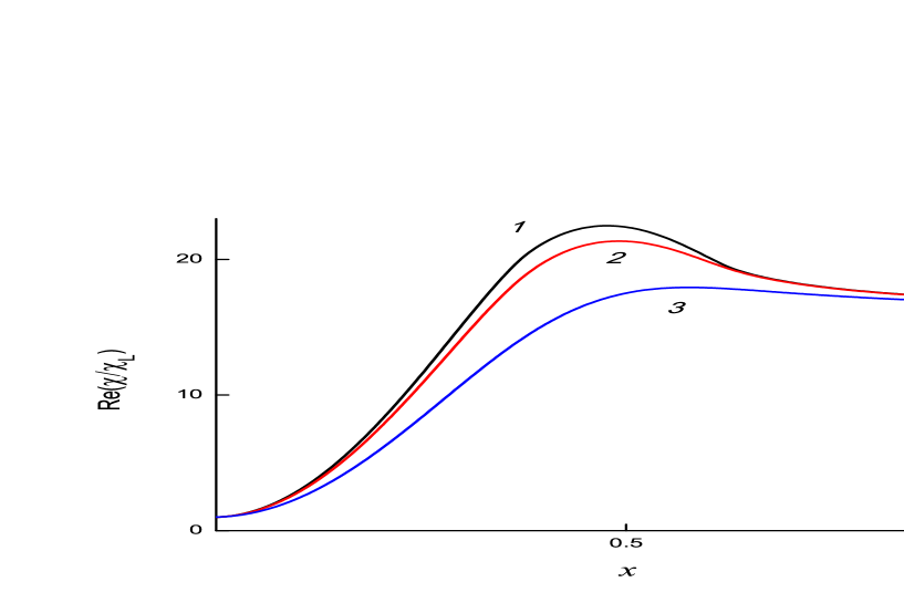
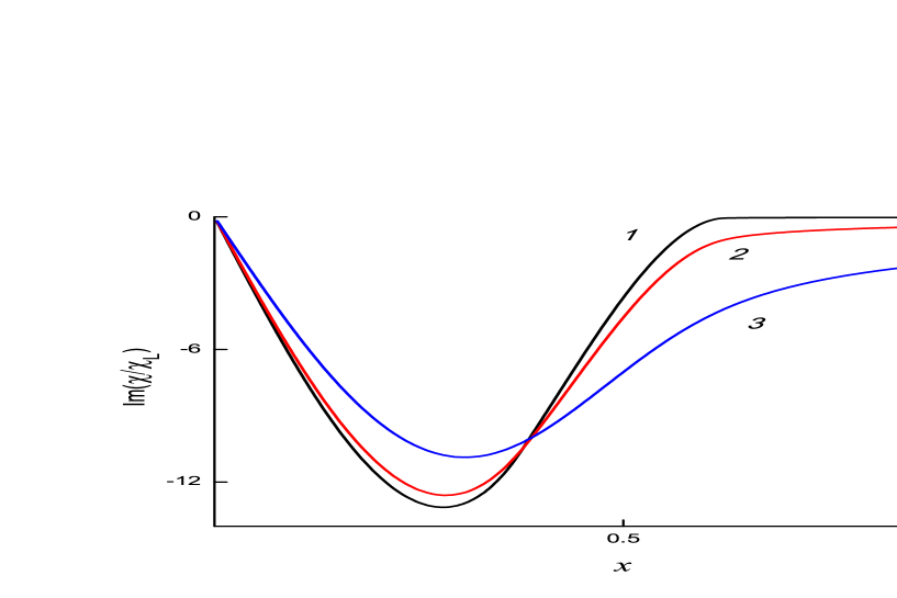
Рис. 4: Real part of diamagnetic susceptibility for case $Q=0.5$, curves $1,2,3$ correspond to parameter values $y=10^{-3},10^{-2},10^{-1}$.

Рис. 5: Imaginary part of diamagnetic susceptibility for case $Q=0.5$, curves $1,2,3$ correspond to parameter values $y=10^{-3},10^{-2},10^{-1}$.

In the present work the kinetic description of magnetic susceptibilities of quantum collisional degenerate plasmas with use before deduced correct formulas for electric conductivity of quantum plasma is given.

Influence of the collisions of plasma particles on the magnetic susceptibility is found out. Thereby the answer to a question on influence is given to the question of dissipation on Landau diamagnetism put in work [4]. For collisionless plasmas with the help the kinetic approach the known formula of Landau diamagnetism is deduced.

REFERENCES

• [1] L. D. Landau and E. M. Lifshitz. Statistical Physics, part 1, Butterworth-Heinemann, Oxford, 1980.
• [2] Yu. L. Klimontovich, V. P. Silin. The spectra of systems of interacting particles and collective energy losses during passage of charged particles through matter// Uspekhi Fiz. Nauk, \No3, 84–114 (1960). In Russian: Uspekhi Fiz. Nauk. 1960. V. 70(2), 247–286 // Physics-Uspekhi (Advances in Physical Sciences)// J. Exp. Theor. Fiz. 23, 151 (1952); The Spectra of Systems of Interacting Particles// In "Plasma Physics" , Ed. J. E. Drummond (McGraw-Hill, New York). 1961. Chap. 2, pp. 35–87.
• [3] K. L. Kliewer, R. Fuchs. Lindhard Dielectric Functions with a Finite Electron Lifetime. Phys. Rev. 181, \No2 (1969), 552–558.
• [4] S. Dattagupta, A. M. Jayannavar and N. Kumar. Landau diamagnetism revisited. Current science. Vol. 80, No. 7, 10 April. 2001. P. 861 –863.
• [5] N. Kumar and K. Vijay Kumar. On Non–zero Classical Diamagnetism: A Surprise. ArXiv:0811.3071v2 [physics. class-ph] 29 Nov 2008.
• [6] A. V. Latyshev and A. A. Yushkanov. Transverse electrical conductivity of a quantum collisional plasma in the Mermin approach // Theor. and Math. Phys., 175(1): 559–569 (2013).
• [7] L. D. Landau and E. M. Lifshitz. Electrodynamics of Continuous Media. Vol. 8. (2ed., Pergamon, 1984), 434 s.