On the high energy spin excitations in the high temperature superconductors: an RVB theory

Abstract

The high energy spin excitation in the high T_c cuprates is studied in the single mode approximation for the $t-t^{\prime}-J$ model. An exact form for the mode dispersion is derived. When the Gutzwiller projected BCS state is used as the variational ground state, a spin-wave-like dispersion of about 2.2$J$ is uncovered along the $\Gamma=(0,0)$ to $\mathrm{M}=(\pi,0)$ line. Both the mode energy and the integrated intensity of the spin fluctuation spectrum are found to be almost doping independent in large doping range, which agrees very well with the observations of recent RIXS measurements. Together with previous studies on the quasiparticle properties of the Gutzwiiler projected BCS state, our results indicate that such a Fermionic RVB theory can provide a consistent description of both the itinerant and the local aspect of electronic excitations in the high T_c cuprates.

The spin dynamics of the high T_c cuprates is a fundamental issue in the study of high T_c superconductivity for two reasons. On the one hand, the superconducting state of the high T_c cuprates is evolved from and is neighbored by an antiferromagnetic ordered insulating state. On the other hand, the d-wave superconduting pairing in the high T_c cuprates is widely believed to be mediated by the antiferromagnetic spin fluctuations. However, after the intensive studies in the last two decades, it remains elusive if the spin dynamics of the high T_c cuprates is more appropriately described by an itinerant or a local picture. In the magnetic ordered parent compounds, both the itinerant and the local picture work well. However, when the static magnetic order is melt by doping, it becomes unclear if the local spins remain their integrity. In the itinerant picture, collective spin fluctuation emerges only when the system is close to magnetic ordering instability and is essential only near the magnetic ordering wave vector. On the other hand, in the local picture, the integrity of the local spin is dictated by the strong local electron correlation. It thus survives even when the system is far away from magnetic instability and when the probing momentum is far away from the magnetic ordering wave vector. Thus, a detection of the high energy spin excitations in momentum regions far away from the ordering wave vector can provide key information on the nature of spin dynamics in the high T_c cuprates.

Most of our understandings on the spin dynamics of the high T_c cuprates are obtained from the inelastic neutron scattering(INS) measurementsFong ; Hayden ; Vignolle ; Hinkov . A universal feature uncovered by these INS studies is the $(\pi,\pi)$ resonance mode in the superconducting state, which is explained successfully in the itinerant picture as a spin exciton mode below the superconducting gap and is taken as a strong support for d-wave pairing. However, as a result of the limited neutron flux, most INS measurements are made around the antiferromagnetic ordering wave vector $\mathrm{Q}=(\pi,\pi)$ and are limited to relatively low excitation energies. Very recently, the situation is changed dramatically as the resonant inelastic X-ray scattering(RIXS) emerges as a powerful way to study the spin dynamics of the high T_c cupratesAment . Together with INS, we are now able to probe the spin excitation spectrum in the high T_c cuprates in a much larger momentum and energy rangeTacon11 ; Vojta ; Dean1201 ; Dean1202 ; Tacon1301 ; Dean1301 ; Dean1302 . A shocking result from these studies is that the high energy spin wave excitation of the parent compounds survives even in the heavily overdoped systems, for which clear signature of electron itineracy(such as well defined Fermi surface, sharp quasiparticle peak and well defined d-wave BCS gap) have been confirmed by other measurements. More specifically, a spin-wave-like dispersive peak is observed in the spin excitation spectrum by RIXS along the $\Gamma=(0,0)$ to $\mathrm{M}=(\pi,0)$ line. Apart from a significant broadening, both the dispersion and the integrated intensity of this peak are found to be almost doping independent below $x=0.4$. Here $x$ is the density of the doped holes.

The observation of robust high energy spin wave excitation in the heavily doped cuprates poses a serious challenge for theoretical understanding of high temperature superconductivity. From the strongly correlated point of view, the appearance of dispersive high energy spin excitation itself is not that surprising, since the local spins remain their integrity in the doped system. The doped charge carriers act only to dilute the existing local spins and to cut short their spatial correlations. At sufficiently short length scale, we should still expect dispersive spin excitations. However, it is highly nontrivial how this behavior can be integrated into a theory which can simultaneously account for the electron itinerancy around the Fermi surface observed by ARPES measurementsDamascelli . For example, in the RPA treatment of the spin dynamicsNorman , the spin collective mode is only well defined around $\mathrm{Q}=(\pi,\pi)$ and is limited to rather low excitation energies. For momentum far away from $\mathrm{Q}=(\pi,\pi)$, the spin fluctuation spectrum is essentially unchanged by the RPA correction and is composed of a broad particle-hole continuum that can extend in energy up to the band width(see supplementary material A for an example). Another important difference between the local and the itinerant picture is about the local spin sum rule. According to the local picture, the spin fluctuation spectrum should satisfy the sum rule of $\int d\mathrm{q}d\omega S(\mathrm{q},\omega)=\frac{3}{4}(1-x)$ as a result of the no double occupancy constraint. This sum rule is important for a correct description of the spin dynamics in the local picture and is violated in the itinerant picture.

The Gutzwiller projected BCS state is generally believed to be a good variational description of the superconducting state of the high T_c cuprates. After the Gutzwiller projection, the no double occupancy constraint and the local spin sum rule are enforced exactly. Previous studies on this state indicate that it offers a rather good account of the single particle excitation around the Fermi surfaceGros ; Yunoki ; Gros06 ; Nave ; Shih ; Yang ; Li2011 . A recent projected RPA calculation on this state also explains well the evolution of the $(\pi,\pi)$ resonance mode with dopingLi2010 . We thus wonder if the same wave function is also consistent with the new observations made by recent RIXS measurements.

In this paper, we calculate the dispersion of the spin excitation in the single mode approximation for the $t-t^{\prime}-J$ model with the Gutzwiller projected BCS state as the variational ground state. The use of the single mode approximation is just the right choice since almost all the observed spectral weight in the RIXS measurements are concentrated in a single broadened peak. We first derive an exact form of the mode dispersion for the $t-t^{\prime}-J$ model in the single mode approximation. We then use the Gutzwiller projected BCS state to evaluate the expectation values involved in the dispersion relation. We find when the observed pairing gap is used in the calculation, a very good agreement with the RIXS observations can be achieved. This indicates that the Fermionic RVB theory based on the Gutzwiller projected BCS state can not only account for the low energy excitation at the energy scale of the pairing gap, but can also provide an accurate description of the local spin correlation of the high T_c cuprates. It thus provides a balanced account of the itinerant and the local aspect of the electronic excitations in the high T_c superconductors.

In the single mode approximation, the spin wave excitation at momentum $\mathrm{q}$ is created by acting on the ground state with the spin density operator $\mathrm{S}^{+}_{\mathrm{q}}$ and has the form

$$|\Psi\rangle_{\mathrm{q}}=\mathrm{S}_{\mathrm{q}}^{+}|\mathrm{G}\rangle,$$ (1)

in which $|\mathrm{G}\rangle$ is the ground state of the system and is assumed to be normalized. The excitation energy of this mode is

$$\Omega_{\mathrm{q}}=\frac{{}_{\mathrm{q}}\langle\Psi|H|\Psi\rangle_{\mathrm{q}}}{{}_{\mathrm{q}}\langle\Psi|\Psi\rangle_{\mathrm{q}}}-\langle\mathrm{G}|H|\mathrm{G}\rangle,$$ (2)

in which $H$ is the Hamiltonian of the system. When the spin fluctuation spectral weight at momentum $\mathrm{q}$ is distributed in a single broadened peak, as is the case observed in RIXS measurements along the $\Gamma$-M lineTacon11 ; Dean1201 ; Dean1202 ; Tacon1301 ; Dean1301 ; Dean1302 , we can also interpret $\Omega_{\mathrm{q}}$ as the center of gravity of this broadened peak. The integrated intensity of this peak is given by the spin structure factor, or

$$I_{\mathrm{q}}=\int d\omega S(\mathrm{q},\omega)=\langle\mathrm{G}|\mathrm{S}_{-\mathrm{q}}^{-}\mathrm{S}_{\mathrm{q}}^{+}|\mathrm{G}\rangle.$$ (3)

Here $S(\mathrm{q},\omega)$ is the spin fluctuation spectrum at momentum $\mathrm{q}$. Thus in the single mode approximation, the spin fluctuation spectrum is totally determined by the ground state wave function.

Following well known procedures, it can be shown that the mode energy $\Omega_{\mathrm{q}}$ can be calculated from the expectation value of the double commutator between the Hamiltonian and the spin density operator in the ground state. More specifically, it is given by

$$\Omega_{\mathrm{q}}=\frac{1}{2}\frac{\langle\mathrm{G}|[\mathrm{S}_{\mathrm{q}}^{-},[\mathrm{S}_{\mathrm{q}}^{+},H]]|\mathrm{G}\rangle}{\langle\mathrm{G}|\mathrm{S}_{\mathrm{q}}^{-}\mathrm{S}_{\mathrm{q}}^{+}|\mathrm{G}\rangle}.$$ (4)

In the derivation, we have assumed that $|\mathrm{G}\rangle$ is the exact ground state of $H$. Now we apply this formula to the $t-t^{\prime}-J$ model of the high T_c cuprates. The Hamiltonian of the model reads

$$H= - t\sum_{<i,j>,\alpha}(\hat{c}_{i,\alpha}^{\dagger}\hat{c}_{j,\alpha}+\mathrm{h.c.})$$ (5)

$$- t^{\prime}\sum_{<<i,j>>,\alpha}(\hat{c}_{i,\alpha}^{\dagger}\hat{c}_{j,\alpha}+\mathrm{h.c.})$$

$$+ J\sum_{<i,j>}(\vec{\mathrm{S}}_{i}\cdot\vec{\mathrm{S}}_{j}-\frac{1}{4}n_{i}n_{j}),$$

in which $\hat{c}_{i,\alpha}=c_{i,\alpha}(1-n_{i,-\alpha})$ is the constrained Fermion operator that satisfies $\sum_{\alpha}\hat{c}_{i,\alpha}^{\dagger}\hat{c}_{i,\alpha}\leq 1$. $\alpha=\pm 1$ is the spin of the electron. $<i,j>$ and $<<i,j>>$ mean nearest and next-nearest neighboring sites. $\vec{\mathrm{S}}_{i}=\frac{1}{2}\sum_{\alpha,\beta}\hat{c}_{i,\alpha}^{\dagger}\vec{\sigma}\hat{c}_{i,\beta}$ and $n_{i}=\sum_{\alpha}\hat{c}_{i,\alpha}^{\dagger}\hat{c}_{i,\alpha}$ are the spin and electron number operators at site $i$. The spin density operator at momentum $\mathrm{q}$ is given by $\mathrm{S}_{\mathrm{q}}^{+}=\sum_{i}e^{i\mathrm{q}\cdot\mathrm{R}_{i}}\mathrm{S}_{i}^{+}$.

To evaluate $\Omega_{\mathrm{q}}$ from Eq.4, we need the commutator between $\mathrm{S}_{\mathrm{q}}^{+}$ and the operators in $H$. It can be shown directly that these commutators are given byLi2010

$$[\hat{c}_{i,\alpha}^{\dagger},\mathrm{S}_{i}^{+}] = -\delta_{\alpha,-1}\hat{c}_{i,+1}^{\dagger}$$

$$[\hat{c}_{i,\alpha},\mathrm{S}_{i}^{+}] = -\delta_{\alpha,+1}\hat{c}_{i,-1}$$

$$[n_{i},\mathrm{S}_{i}^{+}] = 0$$

$$[\mathrm{S}_{i}^{-},\mathrm{S}_{i}^{+}] = -2\mathrm{S}_{i}^{z}$$

$$[\mathrm{S}_{i}^{z},\mathrm{S}_{i}^{+}] = \mathrm{S}_{i}^{+}.$$ (6)

When these commutators are inserted into Eq.4, we find

$$\Omega_{\mathrm{q}}=\frac{3}{8}\frac{(\mathrm{K}+\frac{16}{3}\mathrm{Ex})(1-\gamma(\mathrm{q}))+\mathrm{K}^{\prime}(1-\eta(\mathrm{q}))}{S(\mathrm{q})}.$$ (7)

In the derivation we have assumed that $|\mathrm{G}\rangle$ is spin rotational invariant. In Eq.7,

$$\mathrm{K} = t\langle\mathrm{G}|\sum_{<i,j>,\alpha}(\hat{c}_{i,\alpha}^{\dagger}\hat{c}_{j,\alpha}+\mathrm{h.c.})|\mathrm{G}\rangle$$

$$\mathrm{K^{\prime}} = t^{\prime}\langle\mathrm{G}|\sum_{<<i,j>>,\alpha}(\hat{c}_{i,\alpha}^{\dagger}\hat{c}_{j,\alpha}+\mathrm{h.c.})|\mathrm{G}\rangle$$

$$\mathrm{Ex} = -J\langle\mathrm{G}|\sum_{<i,j>}\vec{\mathrm{S}}_{i}\cdot\vec{\mathrm{S}}_{j}|\mathrm{G}\rangle$$ (8)

are the expectation values of the kinetic energies and the spin exchange energy in $|\mathrm{G}\rangle$. $\gamma(\mathrm{q})=(\cos(\mathrm{q}_{x})+\cos(\mathrm{q}_{y}))/2$ and $\eta(\mathrm{q})=\cos(\mathrm{q}_{x})\cos(\mathrm{q}_{y})$ are the form factors for nearest and next-nearest neighboring hopping terms in the $t-t^{\prime}-J$ model. $S(\mathrm{q})=\sum_{i,j}e^{i\mathrm{q}\cdot(\mathrm{R}_{i}-\mathrm{R}_{j})}\langle\mathrm{G}|\vec{\mathrm{S}}_{i}\cdot\vec{\mathrm{S}}_{j}|\mathrm{G}\rangle$ is the spin structure factor at momentum $\mathrm{q}$.

We thus get a closed form for the mode dispersion for the $t-t^{\prime}-J$ model in the single mode approximation. From Eq.7, it is clear that the dispersion of the mode is mainly determined by the momentum dependence of the spin structure factor $S(\mathrm{q})$, since the expectation values $\mathrm{K}$, $\mathrm{K^{\prime}}$ and $\mathrm{Ex}$ in the nominator are all local quantities that are not sensitive to the exact form of the ground state $|\mathrm{G}\rangle$. For example, an estimate of these quantities to the accuracy of 10 percent can be easily achieved by an ordinary variational wave function. On the other hand, an accurate estimate of the spin structure factor is much more demanding. The RIXS data thus provides important information on the spin correlation in the ground state and may serve as a smoking gun to discriminate between different theories of the high T_c cupartes.

Now we use the Gutzwiller projected BCS state to evaluate the mode energy $\Omega_{\mathrm{q}}$ and the integrated intensity $I_{\mathrm{q}}$ for the high T_c cuprates. It is given by

$$|\mathrm{G}\rangle=\mathrm{P_{G}}|\mathrm{BCS}\rangle,$$ (9)

in which $\mathrm{P_{G}}$ is the projection into the subspace of no double occupancy. $|\mathrm{BCS}\rangle$ is the ground state of the following BCS mean field Hamiltonian

$$H_{\mathrm{MF}}=\sum_{\mathrm{k},\alpha}\epsilon_{\mathrm{k}}c_{\mathrm{k},\alpha}^{\dagger}c_{\mathrm{k},\alpha}+\sum_{\mathrm{k}}\Delta_{\mathrm{k}}(c_{\mathrm{k},+1}^{\dagger}c_{-\mathrm{k},-1}^{\dagger}+\mathrm{h.c.}),$$ (10)

in which $\epsilon_{\mathrm{k}}=-2t_{v}(\cos(\mathrm{k}_{x})+\cos(\mathrm{k}_{y}))-4t^{\prime}_{v}\cos(\mathrm{k}_{x})\cos(\mathrm{k}_{y})+\mu_{v}$, $\Delta_{k}=\Delta_{v}(\cos(\mathrm{k}_{x})-\cos(\mathrm{k}_{y}))$. Here $t^{\prime}_{v}/t_{v}$, $\mu_{v}/t_{v}$ and $\Delta_{v}/t_{v}$ should be understood as variational parameters to be determined by energy optimization. This can be done with the standard variational Monte Carlo methodGros .

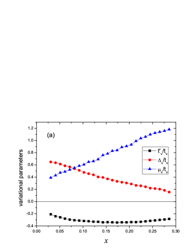
Figure 1: (a)The doping dependence of the optimized variational parameters in the Gutzwiller projected BCS state. (b)The doping dependence of $\frac{v_{\Delta}}{v_{\mathrm{F}}}$ at the nodal point as determined from the optimized variational parameters.

Our calculation is done on a $14\times 14$ lattice. We have adopted the periodic-antiperiodic boundary condition to avoid the d-wave node. In the calculation, we have set $t^{\prime}=-0.25t$ and $J=t/3$, as is usually assumed in the literature. The values of the optimized variational parameters are shown in Fig.1a as functions of doping. For later reference, we also plot in Fig.1b the ratio between the gap slope $v_{\Delta}$ and the Fermi velocity $v_{\mathrm{F}}$ at the nodal point as determined from the optimized variational parameters. Here the gap slope is defined as $v_{\Delta}=|\frac{\partial\Delta_{\mathrm{k}}}{\partial\mathrm{k}}|$. At the nodal point on the Fermi surface, it can be shown that $v_{\Delta}=\frac{\Delta_{v}}{2\sqrt{t_{v}^{2}+\mu_{v}t^{\prime}_{v}}}$.

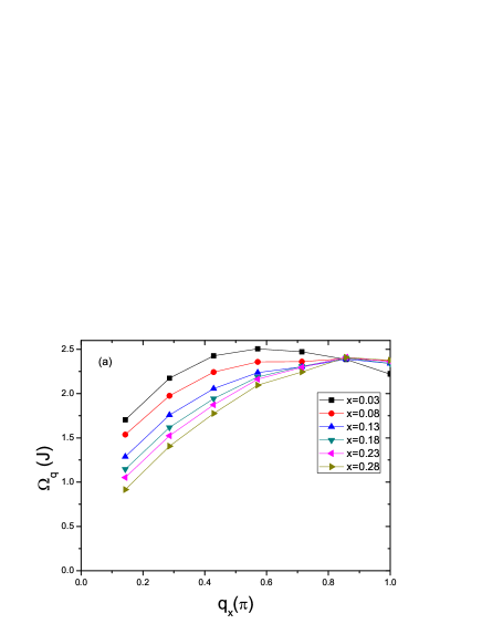
Figure 2: The dispersion of the mode energy $\Omega_{\mathrm{q}}$ along the $\Gamma$-M line. Here $\mathrm{q}_{y}$ is fixed at zero. In (a), we have used the pairing gap determined from variational optimization. In (b), we have divided the variational pairing gap by a factor of 4 so as to match the observed value of $\frac{v_{\Delta}}{v_{\mathrm{F}}}\sim\frac{1}{20}$ around $x=0.15$Campuzano ; Mesot ; Chiao .

The doping dependence of the mode energy $\Omega_{\mathrm{q}}$ along the $\Gamma$-M line calculated with the optimized variational parameters is shown in Fig.2a. The overall energy scale of the mode dispersion along the $\Gamma$-M line is about $2J$, which is quite consistent with the observation in RIXS measurements if we assume $J=125$ meVDean1201 . However, the doping dependence of the dispersion is rather strong and is inconsistent with the experimental observations. In particular, the mode energy is found to increase with decreasing doping at small $\mathrm{q}$ and deviates strongly from the linear spin wave dispersion around the $\Gamma$ point at small doping. Such a discrepancy indicates that certain features in the spin correlation of the high T_c cuprates is not correctly captured by the Gutzwiller projected BCS state if the optimized variational parameters are used.

To see the origin of such a discrepancy, we note the dispersion of $\Omega_{\mathrm{q}}$ is solely determined by the spin structure factor $S(\mathrm{q})$. In the long wave length limit, both $1-\gamma(\mathrm{q})$ and $1-\eta(\mathrm{q})$ in the nominator of Eq.7 behave as quadratic functions of momentum. The coefficients of $1-\gamma(\mathrm{q})$ and $1-\eta(\mathrm{q})$, namely $\mathrm{K+\frac{16}{3}Ex}$ and $\mathrm{K^{\prime}}$, are all local quantities and can both be estimated accurately from the variational ground state. To reproduce the linear dispersion in the long wave length limit, the spin structure factor must be linear in $\mathrm{q}$ in the same limit. This is just what we expect in a Fermi liquid with a nonzero density of state on the Fermi surface. More specifically, the spin structure factor in a Fermi gas is given by $S(\mathrm{q})=\frac{2}{3}\sum_{\mathrm{k}}\Theta(\epsilon_{\mathrm{k+q}})(1-\Theta(\epsilon_{\mathrm{k}}))$, in which $\epsilon_{\mathrm{k}}$ is the dispersion of the Fermion. In the long wavelength limit, only those states that are within a shell of thickness proportional to $\mathrm{q}$ around the Fermi surface can contribute to $S(\mathrm{q})$, which is thus proportional to both $\mathrm{q}$ and the density of state at the Fermi energy. On the other hand, in the superconducting state, the low energy spin excitation is gapped out by the superconducting gap and the spin structure factor is given by

$$S(\mathrm{q})=\frac{1}{2}\sum_{\mathrm{k}}(1-\frac{\epsilon_{\mathrm{k}}\epsilon_{\mathrm{k+q}}+\Delta_{\mathrm{k}}\Delta_{\mathrm{k+q}}}{E_{\mathrm{k}}E_{\mathrm{k+q}}}),$$ (11)

in which $E_{\mathrm{k}}=\sqrt{\epsilon^{2}_{\mathrm{k}}+\Delta^{2}_{\mathrm{k}}}$. In the long wavelength limit, the BCS coherence factor $(1-\frac{\epsilon_{\mathrm{k}}\epsilon_{\mathrm{k+q}}+\Delta_{\mathrm{k}}\Delta_{\mathrm{k+q}}}{E_{\mathrm{k}}E_{\mathrm{k+q}}})$ is suppressed quadratically as a result of the singlet pairing. Thus the spin structure factor $S(\mathrm{q})$ is a quadratic function of momentum for small $\mathrm{q}$. We find the above argument also apply to the Gutzwiller projected BCS state. This explains why $\Omega_{\mathrm{q}}$ is gapped at the $\Gamma$ point for small $x$ in Fig.2a.

With these understandings, we now improve the variational ground state. For this purpose, we note the pairing gap as determined from the variational theory is actually much larger than that observed in experiments. More specifically, both ARPES and transport measurement find that $\frac{v_{\Delta}}{v_{\mathrm{F}}}\sim\frac{1}{20}$ at the optimal dopingCampuzano ; Mesot ; Chiao , while the value of $\frac{v_{\Delta}}{v_{\mathrm{F}}}$ determined from the optimized variational parameters is about 0.2 for $x=0.15$(see Fig.1b). Thus, the observed contour of equal energy around the gap node is about a factor of 4 more anisotropic than that predicted by the variational theory. For this reason, we scale down the size of the pairing gap by a factor of four so as to match the observed value of $\frac{v_{\Delta}}{v_{\mathrm{F}}}$. The mode energy calculated with the rescaled pairing gap is shown in Fig.2b, which is seen to be much more consistent with the dispersion reported in RIXS measurements. In particular, the doping dependence of mode dispersion becomes now very weak and an approximate linear dispersion is recovered in the long wavelength limit. The overall scale of the dispersion is about 2.2$J$. This also agrees well with the RIXS data if we assume $J=125$ meV.

In Fig.3, we plot the doping dependence of the integrated mode intensity $I_{\mathrm{q}}$ along the $\Gamma$-M line. We find $I_{\mathrm{q}}$ is almost independent of the doping along the whole $\Gamma$-M line. This is consistent with the observation of RIXS measurements. However, we note $I_{\mathrm{q}}$ is strongly doping dependent around the antiferromagnetic ordering wave vector $\mathrm{Q}=(\pi,\pi)$(see the supplementary material B).

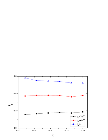
Figure 3: The doping dependence of the integrated intensity of the spin fluctuation spectrum along the $\Gamma$-M line. The parameters used here are the same as that used in Fig.2b.

Thus, the main observations of the RIXS measurements can be well explained by the Fermionic RVB theory, if the observed pairing gap, rather than that determined from variational optimization, is adopted. Together with the results of extensive studies on the quasiparticle properties of the Gutzwiller projected BCS state, our results indicate that the Fermionic RVB theory can not only provide a consistent understanding on the low energy excitations around the Fermi surface, but can also provide an accurate description of the local physics of the high-T_c cuprates. The Fermionic RVB theory is thus a promising framework to unify both the itinerant and the local aspect of electronic excitations in these doped Mott insulators. Nevertheless, the RIXS data remind us again that the pairing gap is overestimated substantially in the standard Fermionic RVB theory. This overestimation is most likely caused by the insufficient account of the antiferromagnetic spin fluctuation in the Fermionic RVB theory, which competes with the tendency of spin singlet pairing. This is reasonable since both the antiferromagnetic spin fluctuation and the d-wave spin singlet pairing are driven by the same spin superexchange interaction in the $t-t^{\prime}-J$ Hamiltonian. A more advanced theory of the high T_c cuprates should of course treat both ordering tendencies on the same footing.

Finally, we note the single mode approximation becomes less useful around $\mathrm{Q}=(\pi,\pi)$, as the spin fluctuation spectrum develops finer structures in this momentum regionVignolle ( Supplementary material B contains a more detailed discussion on this point). A general approach to study these structures in the Fermionic RVB theory is proposed recently by usLi2010 . It is interesting to apply this approach to the high T_c cuprates to arrive at a deeper understanding of such a strongly correlated system.

This work is supported by NSFC Grant No. 10774187, No. 11034012 and National Basic Research Program of China No. 2010CB923004.

I Supplementary materials

I.1 The spin fluctuation spectrum of the high T_c cuprates in the itinerant picture

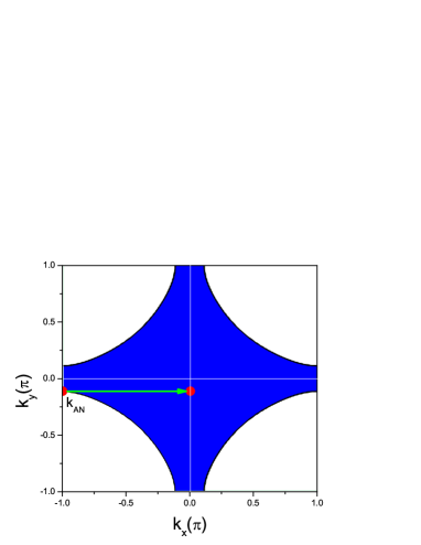
Figure 4: The Fermi surface of the tight-binding model we used to calculate the mean field spin susceptibility $\chi^{0}(\mathrm{q},\omega)$. The arrow and the red dots illustrate the transition at the peak energy for $\mathrm{q}=(\pi,0)$.

To check if the RIXS data is consistent with an itinerant picture, we have calculated the spin fluctuation spectrum of the cuprates from the random phase approximation. In the RPA scheme, the dynamic spin susceptibility is given by

$$\chi(\mathrm{q},\omega)=\frac{\chi^{0}(\mathrm{q},\omega)}{1+J(\mathrm{q})\chi^{0}(\mathrm{q},\omega)},$$ (12)

in which $\chi^{0}(\mathrm{q},\omega)$ is the bare spin susceptibility of the band electron and $J(\mathrm{q})=J(\cos(\mathrm{q}_{x})+\cos(\mathrm{q}_{y}))$ is the RPA kernel caused by the antiferromagnetic spin exchange. The bare susceptibility $\chi^{0}(\mathrm{q},\omega)$ in the BCS superconducting state is given by

$$\chi^{0}(\mathrm{q},\omega) = \frac{1}{4}\sum_{\mathrm{k}}(1-\frac{\epsilon_{\mathrm{k}}\epsilon_{\mathrm{k+q}}+\Delta_{\mathrm{k}}\Delta_{\mathrm{k+q}})}{E_{\mathrm{k}}E_{\mathrm{k+q}}})$$ (13)

$$\times (\frac{1}{\omega-E_{\mathrm{k}}-E_{\mathrm{k+q}}+i0^{+}}$$

$$- \frac{1}{\omega+E_{\mathrm{k}}+E_{\mathrm{k+q}}+i0^{+}}),$$

in which $\epsilon_{\mathrm{k}}=-2t(\cos(\mathrm{k}_{x})+\cos(\mathrm{k}_{y}))-4t^{\prime}\cos(\mathrm{k}_{x})\cos(\mathrm{k}_{y})-\mu$ is the band dispersion and $\Delta_{\mathrm{k}}=\Delta(\cos(\mathrm{k}_{x})-\cos(\mathrm{k}_{y}))$ is the BCS gap function. The parameters $t$, $t^{\prime}$ and $\mu$ can be determined by fitting the ARPES results. Here we set $t=250$ meV, $t^{\prime}=-0.3t$, $\mu=-t$. The Fermi surface for this set of parameters is plotted in Fig.4, which corresponds to a doping of $x=0.15$ and is very similar to that observed in the optimally doped $Bi_{2}Sr_{2}CaCu_{2}O_{8+\delta}$Damascelli . We also set $\Delta=25$ meV, so that $\frac{v_{\Delta}}{v_{\mathrm{F}}}\approx\frac{1}{20}$. We note that the conclusion of this section is not sensitive to the exact values of these parameters.

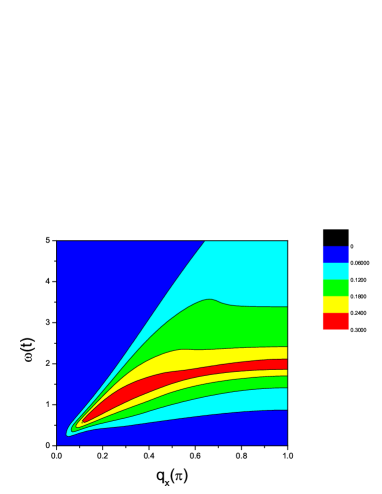
Figure 5: A color map of the mean field spin fluctuation spectrum along the $\Gamma$-M line. Here $\mathrm{q}_{y}$ is fixed at zero.

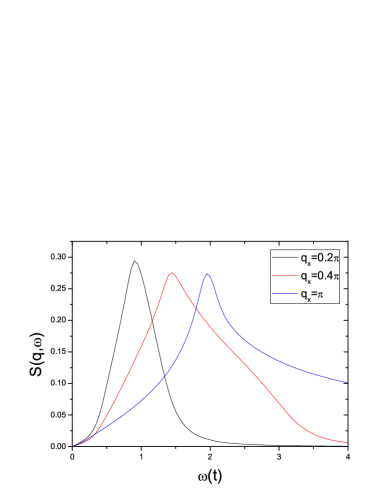
Figure 6: The mean field spin fluctuation spectrum at three momentums along the $\Gamma$-M line.

The bare spin fluctuation spectrum(the imaginary part of $\chi^{0}(\mathrm{q},\omega)$)is composed of a continuum of the particle-hole excitations. The RPA correction, which is responsible for the emergence of soft collective mode around the antiferromagnetic ordering wave vector $\mathrm{Q}=(\pi,\pi)$, has a much weaker effect along the $\Gamma$-M line as is probed in the RIXS measurements. In particular, the RPA correction can not introduce any new pole in this momentum region. For clarity, we will only present the mean field spectrum. The result is shown in Fig.5. For small $\mathrm{q}_{x}$, the continuum is bounded above by $v^{m}_{\mathrm{F},x}\mathrm{q}_{x}$, in which $v^{m}_{\mathrm{F},x}$ is the maximal Fermi velocity in the $x$ direction on the Fermi surface. At the M point, the continuum becomes as broad as the whole band.

A prominent feature in the mean field spectrum is the dispersive peak inside the continuum. To understand its origin, we plot in Fig.6 the spectrum at several momentum along the $\Gamma$-M line. The peak is found to be related to the Van Hove singularity in the particle-hole continuum. For $\mathrm{q}$=M, this peak corresponds to the transition from the antinodal point on the Fermi surface to momentum around the band bottom. This is illustrated in Fig.4. The peak energy at the M point is given by $E^{peak}_{\mathrm{q}=\mathrm{M}}\approx E_{\mathrm{k}=\mathrm{k_{AN}}}+E_{\mathrm{k}=0}=|\Delta|+4(t+t^{\prime})+\mu$. Here $\mathrm{k_{AN}}$ is the momentum of the antinodal point. For the parameters we have used, $E^{peak}_{\mathrm{q}=\mathrm{M}}\approx 2t$. Although the dispersion of this peak looks similar to that observed in RIXS measurements, the energy of the peak is much higher than that observed. Furthermore, the peak width is also too broad to be consistent with experiment. Taken as a whole, the itinerant picture predicts a broad continuum and a significantly higher energy scale for spin excitation along the $\Gamma$-M line. The itinerant picture is thus inconsistent with the RIXS data.

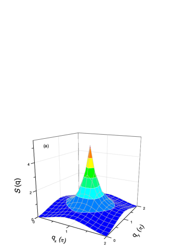
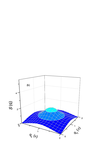
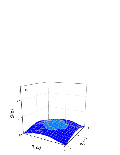
Figure 7: The spin structure factor at $x=0.03$(a), $x=0.16$(b) and $x=0.28$(c).

I.2 The spin fluctuation spectrum in other region of the Brillouin zone

From our calculation, we see both the dispersion and the integrated intensity of the spin excitation spectrum are almost doping independent along the $\Gamma$-M line. However, this is not generally true in other regions of the Brillouin zone. In particular, the spin fluctuation spectrum around the anfiferromagnetic ordering wave vector $\mathrm{Q}=(\pi,\pi)$ is strongly doping dependent. In Fig.7, we plot the spin structure factor for $x=0.03$, $0.16$ and $0.28$. A strong peak at $\mathrm{Q}=(\pi,\pi)$ is found for $x=0.03$, which diminishes rapidly with increasing doping. The doping dependence of the spin structure factor at $\mathrm{Q}=(\pi,\pi)$ is shown in Fig.8.

Figure 8: The doping dependence of the spin structure factor at $\mathrm{Q}=(\pi,\pi)$.

Apart from the integrated intensity, the center of gravity of the spin fluctuation spectrum is also strongly doping dependent around $(\pi,\pi)$. In Fig.9, we plot the dispersion of $\Omega_{\mathrm{q}}$ along the the M-Q line. Around $\mathrm{Q}=(\pi,\pi)$, $\Omega_{\mathrm{q}}$ is found to increase rapidly with doping and reaches 2$J$ at $x=0.28$. In this region of the momentum space, the spin fluctuation spectrum develops multi-component structureVignolle and the single mode approximation becomes less useful. The large value of $\Omega_{\mathrm{q}}$ nevertheless indicates that a large amount of spin fluctuation spectral weight at $\mathrm{q}=(\pi,\pi)$ is distributed in a broad range of energy of the order of 2$J$ in the overdoped systems. It would be quite challenging for both INS and RIXS to detect such strongly smeared-out spectral weight.

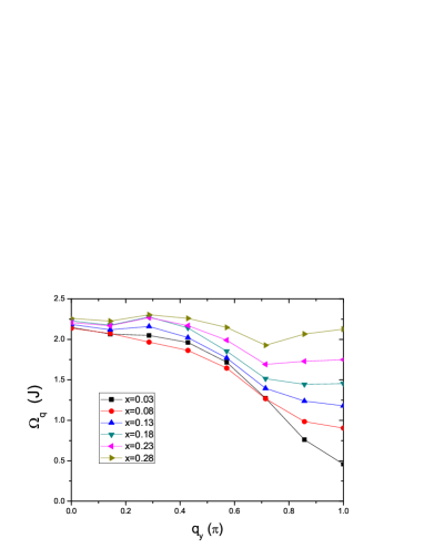
Figure 9: The dispersion of $\Omega_{\mathrm{q}}$ along the M-Q line. Here $\mathrm{q}_{x}$ is fixed at $\pi$.

References

- (1) H. F. Fong, B. Keimer, P. W. Anderson, D. Reznik, F. Dogan, and I. A. Aksay, Phys. Rev. Lett. 75, 316 1995.
- (2) S.M. Hayden, H.A. Mook, P. Dai, T.G. Perring, and F. Dogan, Nature 429, 531 (2004).
- (3) B. Vignolle, S. M. Hayden, D. F. McMorrow, H. M. Rønnow, B. Lake, C. D. Frost and T. G. Perring, Nature Phys. 3, 163 (2007).
- (4) V. Hinkov, P. Bourges, S. Pailhès, Y. Sidis, A. Ivanov, C. D. Frost, T. G. Perring, C. T. Lin, D. P. Chen and B. Keimer Nature Physics 3, 780 (2007).
- (5) L. J. P. Ament, M. van Veenendaal, T. P. Devereaux, J. P. Hill, and J. van den Brink, Rev. Mod. Phys. 83, 705 (2011).
- (6) M. Le Tacon, G. Ghiringhelli, J. Chaloupka, M. M. Sala, V. Hinkov, M. W. Haverkort, M. Minola, M. Bakr, K. J. Zhou, S. Blanco-Canosa, C. Monney, Y. T. Song, G. L. Sun, C. T. Lin, G. M. De Luca, M. Salluzzo, G. Khaliullin, T. Schmitt, L. Braicovich, and B. Keimer, Nat. Phys. 7, 725 (2011).
- (7) M. Vojta, Nature Phys. 7, 674 (2011).
- (8) M. P. M. Dean, R. S. Springell, C. Monney, K. J. Zhou, J. Pereiro, I. Božović, B. Dalla Piazza, H. M. Rønnow, E. Morenzoni, J. van den Brink, T. Schmitt, and J. P. Hill, Nat. Mater. 11, 850 (2012).
- (9) M. P. M. Dean, A. J. A. James, R. S. Springell, X. Liu, C. Monney, K. J. Zhou, R. M. Konik, J. S. Wen, Z. J. Xu, G. D. Gu, V. N. Strocov, T. Schmitt, and J. P. Hill, Phys. Rev. Lett. 110, 147001 (2013).
- (10) M. Le Tacon, M. Minola, D. C. Peets, M. Moretti Sala, S. Blanco-Canosa, V. Hinkov, R. Liang, D. A. Bonn, W. N. Hardy, C. T. Lin, T. Schmitt, L. Braicovich, G. Ghiringhelli, and B. Keimer, arXiv:1303.3947 (2013).
- (11) M. P. M. Dean, G. Dellea, R. S. Springell, F. Yakhou- Harris, K. Kummer, N. B. Brookes, X. Liu, Y.-J. Sun, J. Strle, T. Schmitt, L. Braicovich, G. Ghiringhelli, I. Bozovic, and J. P. Hill, arXiv:1303.5359 (2013).
- (12) M. P. M. Dean, G. Dellea, M. Minola, S. B. Wilkins, R. M. Konik, G. D. Gu, M. Le Tacon, N. B. Brookes, F. Yakhou-Harris, K. Kummer, J. P. Hill, L. Braicovich, and G. Ghiringhelli, arXiv:1305.1317.
- (13) A. Damascelli, Z. X. Shen, and Z. Hussain, Rev. Mod. Phys. 75, 473 (2003).
- (14) M. R. Norman, Phys. Rev. B 61, 14751 (2000).
- (15) B. Edegger, V. N. Muthukumar, and C. Gros, Adv. Phys. 56, 927 (2007).
- (16) S. Yunoki, E. Dagotto, and S. Sorella, Phys. Rev. Lett. 94, 037001 (2005).
- (17) C. Gros, B. Edegger, V. N. Muthukumar, and P. W. Anderson, Proc. Natl. Acad. Sci. USA 103, 14298 (2006);B. Edegger, V. N. Muthukumar, C. Gros, and P. W. Anderson, Phys. Rev. Lett. 96, 207002 (2006); B. Edegger, N. Fukushima, C. Gros, and V. N. Muthukumar, Phys. Rev. B 72, 134504 (2005).
- (18) C. P. Nave, D. A. Ivanov, and P. A. Lee, Phys. Rev. B 73, 104502 (2006).
- (19) C. T. Shih, T. K. Lee, R. Eder, C. Y. Mou, and Y. C. Chen, Phys. Rev. Lett. 92, 227002 (2004).
- (20) H. Y. Yang, F. Yang, Y. J. Jiang, and T. Li, J. Phys. C 19, 016217 (2007).
- (21) F. Yang and T. Li, Phys. Rev. B 83, 64524 (2011).
- (22) T. Li and F. Yang, Phys. Rev. B 81, 214509 (2010).
- (23) J. C. Campuzano, M. R. Norman, M. Randeria, in ”Physics of Superconductors”, Vol. II, ed. K. H. Bennemann and J. B. Ketterson (Springer, Berlin, 2004), p. 167-273.
- (24) J. Mesot, M. R. Norman, H. Ding, M. Randeria, J. C. Campuzano, A. Paramekanti, H. M. Fretwell, A. Kaminski, T. Takeuchi, T. Yokoya, T. Sato, T. Takahashi, T. Mochiku, and K. Kadowaki, Phys. Rev. Lett. 83 , 840 (1999).
- (25) M. Chiao, P. Lambert, R. W. Hill, C. Lupien, R. Gagnon, L. Taillefer, P. Fournier, Phys. Rev. B 62 , 3554 (2000).