On charged boson stars

Abstract

We study static, spherically symmetric, self-gravitating systems minimally coupled to a scalar field with $U(1)$ gauge symmetry: charged boson stars. We find numerical solutions to the Einstein-Maxwell equations coupled to the relativistic Klein-Gordon equation. It is shown that bound stable configurations exist only for values of the coupling constant less than or equal to a certain critical value. The metric coefficients and the relevant physical quantities such as the total mass and charge, turn out to be in general bound functions of the radial coordinate, reaching their maximum values at a critical value of the scalar field at the origin. We discuss the stability problem both from the quantitative and qualitative point of view. Taking properly into account the electromagnetic contribution to the total mass, the stability issue is faced also following an indication of the binding energy per particle, verifying then the existence of configurations having positive binding energy: objects apparently bound can be unstable against small perturbations, in full analogy with what observed in the mass-radius relation of neutron stars.

I Introduction

Spherically symmetric charged boson stars are solutions of the Einstein-Maxwell system of equations coupled to the general relativistic Klein-Gordon equations of a complex scalar field with a local $U(1)$ symmetry. The study of the phenomena related to the formation and stability of self-gravitating systems is of major interest in astrophysics. It has been conjectured, for instance, that a boson star could model Bose-Einstein condensates on astrophysical scales SM99 ; SM98 ; MS96 ; JS94 ; JB01 ; BLV01 ; JoBern2001 ; ChaHar2012 . The collapse of charged compact objects composed by bosons could lead in principle to charged black holes (see e.g. Jetzer:1993nk ; Kleihaus:2009kr and also TCL00 ). Compact boson objects play an important role in astrophysics since these configurations may represent also an initial condition for the process of gravitational collapse RR2007 ; see also Lieb-Pale12 for a recent review. Moreover, boson stars have been shown to be able to mimic the power spectrum of accretion disks around black holes (see, for example, Guzman-RUBE2009 ). Scalar fields are also implemented in many cosmological models either to regulate the inflationary scenarios Gorini:2003wa ; LlinMota13 ; Bertolami:2004nh ; Fay04 or to describe dark matter and dark energy (see e.g. BerCarPar2012 ; GaoKinkLiPar10 ; MainColoBono05 ; Arbey09 ). On the other hand, in the Glashow-Weinberg-Salam Standard Model of elementary particles, a real scalar particle, the Higgs boson, is introduced in order to provide leptons and vector bosons with mass after symmetry breaking; in this respect, the latest results of the Large Hadron Collider experiments Chatrchyan:2012ufa reflect the importance of the scalar fields in particle physics. Scalar fields are also found within superstring theories as dilaton fields, and, in the low energy limit of string theory, give rise to various scalar-tensor theories for the gravitational interaction polchinski .

Ruffini and Bonazzola RR quantized a real scalar field and found a spherically symmetric solution of the Einstein-Gordon system of equations. The general relativistic treatment eliminates completely some difficulties of the Newtonian approximation, where an increase of the number of particles corresponds to an increase of the total energy of the system until the energy reaches a maximum value and then decreases to assume negative values. It was also shown in RR that for these many boson systems the assumption of perfect fluid does not apply any longer since the pressure of the system is anisotropic. On the other hand, this treatment introduces for the first time the concept of a critical mass for these objects. Indeed, in full analogy with white dwarfs and neutron stars, there is a critical mass and a critical number of particles and, for charged objects, a critical value of the total charge, over which this system is unstable against gravitational collapse to a black hole.

In Jetzer:1989av ; Jetzer:1989us ; Jetzer:1990wr the study of the charged boson stars was introduced solving numerically the Einstein-Maxwell-Klein-Gordon equations. In Jetzer:1989us charged boson configurations were studied for non singular asymptotically-flat solutions. In particular, it was shown the existence of a critical value for the central density, mass and number of particles. The gravitational attraction of spherically symmetric self-gravitating systems of bosons (charged and neutral) balances the kinetic and Coulomb repulsion. On the other hand, the Heisenberg uncertainty principle prevents neutral boson stars from a gravitational collapse. Furthermore, in order to avoid gravitational collapse the radius $R$ must satisfy the condition $R\geq 3R_{\mbox{\tiny{S}}}$ where $R_{\mbox{\tiny{S}}}$ is Schwarzschild radius Schunck:2003kk ; Jetzer:1989fx . On the other hand, stable charged boson stars can exist if the gravitational attraction is larger than the Coulomb repulsion: if the repulsive Coulomb force overcomes the attractive gravitational force, the system becomes unstable Schunck:2003kk ; Jetzer:1991jr ; Kusmartsev:2008py ; Schunck:1999pm ; Mielke:1997re . Moreover, as for other charged objects, if the radius of these systems is less than the electron Compton wavelength and if they are super–critically charged, then pair production of electrons and positrons occurs.

These previous works restricted the boson charge to the so-called “critical” value (in Lorentz-Heaviside units) $q_{\mbox{\tiny{crit}}}^{2}=4\pi\left(m/M_{\mbox{\tiny{Pl}}}\right)^{2}$ for a particle of mass $m$ where $M_{\mbox{\tiny{Pl}}}$ is the Planck mass. This value comes out from equating the Coulomb and gravitational forces, so it is expected that for a boson charge $q>q_{\mbox{\tiny{crit}}}$, the repulsive Coulomb force be larger than the attractive gravitational one. However, such a critical particle charge does not take into account the gravitational binding energy per particle and so there may be the possibility of having stable configurations for bosons with $q>q_{\mbox{\tiny{crit}}}$.

Thus, in this work we numerically integrate the coupled system of Einstein-Maxwell-Klein-Gordon equations, focusing our attention on configurations characterized by a value of the boson charge close to or larger than $q_{\mbox{\tiny{crit}}}$. We will not consider the excited state for the boson fields, consequently we study only the zero-nodes solutions.

We here show that stable charged configurations of self-gravitating charged bosons are possible with particle charge $q=q_{\mbox{\tiny{crit}}}$. In addition, it can be shown by means of numerical calculations that for values $q>q_{\mbox{\tiny{crit}}}$ localized solutions are possible only for values of the central density smaller than some critical value over which the boundary conditions at the origin are not satisfied. We also study the behavior of the radius as well as of the total charge and mass of the system for $q\simeq q_{\mbox{\tiny{crit}}}$.

The plan of the paper is the following: In Sec. II, we set up the problem by introducing the general formalism and writing the system of Einstein-Maxwell-Klein-Gordon equations for charged boson stars. In Sec. III, we discuss the concepts of charge, radius, mass and particle number. In Sec. IV, we show the results of the numerical integration. Finally, in Sec. V, we summarize and discuss the results. To compare our results with those of uncharged configurations, we include in the Appendix the numerical analysis of the limiting case of neutral boson stars.

II The Einstein-Maxwell-Klein-Gordon equations

We consider static, spherically symmetric self-gravitating systems of a scalar field minimally coupled to a $U(1)$ gauge field: charged boson stars. The Lagrangian density of the massive electromagnetically coupled scalar field $\Phi$, in units with $\hbar=c=1$, is

$$\mathcal{L}_{\mbox{\tiny{M}}}=\sqrt{-g}\left[g^{\mu\nu}\left(D_{\mu}\Phi\right)\left(D_{\nu}\Phi\right)^{*}-m^{2}\Phi\Phi^{*}-\frac{1}{4}F_{\mu\nu}F^{\mu\nu}\right],$$ (1)

where $g\equiv\det g_{\mu\nu}$, $m$ is the scalar field mass and $D_{\mu}\equiv\nabla_{\mu}+\imath qA_{\mu}$, where the constant $q$ is the boson charge, $\nabla$ stands for the covariant derivative, the asterisk denotes the complex conjugation, $A_{\mu}$ is the electromagnetic vector potential, while $F_{\mu\nu}=\partial_{\mu}A_{\nu}-\partial_{\nu}A_{\mu}$ is the electromagnetic field tensor Jetzer:1990wr ; Fulling ; BD . We use a metric $g_{\mu\nu}$ with signature $(+,-,-,-)$; Greek indices run from 0 to 3, while Latin indices run from 1 to 3.

Therefore the total Lagrangian density $\mathcal{L}$ for the field $\Phi$ minimally coupled to gravity and to a $U(1)$ gauge field is

$$\mathcal{L}=\sqrt{-g}\frac{R}{16\pi G_{\mbox{\tiny{N}}}}+\mathcal{L}_{\mbox{\tiny{M}}},$$ (2)

where $R$ is the scalar curvature, $M_{\mbox{\tiny{Pl}}}=G_{\mbox{\tiny{N}}}^{-1/2}$ is the Planck mass, and $G_{\mbox{\tiny{N}}}$ is the gravitational constant.

The Lagrangian density is invariant under a local $U(1)$ gauge transformation (of the field $\Phi$). The corresponding conserved Noether density current $J^{\mu}$ is given by

$$J^{\mu}=\sqrt{-g}g^{\mu\nu}\left[\imath q\left(\Phi^{*}\partial_{\nu}\Phi-\Phi\partial_{\nu}\Phi^{*}\right)-2q^{2}A_{\nu}\Phi\Phi^{*}\right],$$ (3)

while the energy-momentum tensor $T_{\mu\nu}$ is

$$T_{\mu\nu}=\left(D_{\mu}\Phi\right)^{*}\left(D_{\nu}\Phi\right)+\left(D_{\mu}\Phi\right)\left(D_{\nu}\Phi\right)^{*}-g_{\mu\nu}g^{\alpha\beta}\left(D_{\alpha}\Phi\right)^{*}\left(D_{\beta}\Phi\right)$$

$$-g_{\mu\nu}m^{2}\Phi\Phi^{*}+\frac{1}{4}g_{\mu\nu}F_{\alpha\beta}F^{\alpha\beta}-g^{\alpha\beta}F_{\mu\alpha}F_{\nu\beta}.$$ (4)

In the case of spherical symmetry, the general line element can be written in standard Schwarzschild-like coordinates $(t,r,\vartheta,\varphi)$ as

$$ds^{2}=e^{\nu}dt^{2}-e^{\lambda}dr^{2}-r^{2}\left(d\vartheta^{2}+\sin\vartheta^{2}d\varphi^{2}\right),$$ (5)

where $\nu$ and $\lambda$ are functions of the radial coordinate $r$ only. Since we want to study only static solutions, the metric and energy-momentum tensor must be time-independent even if the matter field $\Phi$ may depend on time.

Then, we set the following stationarity ansatz Ad02 ; De64 ; Schunck:2003kk ; Jetzer:1997zx ; Wy81

$$\Phi(r,t)=\phi(r)e^{\imath\omega t},$$ (6)

where $\phi$ is in general a complex field. Equation (6) describes a spherically symmetric bound state of scalar fields with positive (or negative) frequency $\omega$. Accordingly, the electromagnetic four-potential is $A_{\mu}(r)=\left(A_{t}(r)=A(r),A_{r}=0,A_{\theta}=0,A_{\varphi}=0\right)$.

From Eq. (4) we obtain the following non-zero components of the energy-momentum tensor $T^{\mu}_{\phantom{\ }\nu}$:

$$T^{0}_{\phantom{\ }0} = \left[m^{2}+e^{-\nu}\left(\omega+qA\right)^{2}\right]\phi^{2}+\frac{e^{-\lambda-\nu}(A^{\prime})^{2}}{2}+\phi^{\prime 2}e^{-\lambda},$$ (7)

$$T^{1}_{\phantom{\ }1} = \left[m^{2}-e^{-\nu}\left(\omega+qA\right)^{2}\right]\phi^{2}+\frac{e^{-\lambda-\nu}(A^{\prime})^{2}}{2}-\phi^{\prime 2}e^{-\lambda},$$ (8)

$$T^{2}_{\phantom{\ }2} = T^{3}_{\phantom{\ }3}=\left[m^{2}-e^{-\nu}\left(\omega+qA\right)^{2}\right]\phi^{2}-\frac{e^{-\lambda-\nu}(A^{\prime})^{2}}{2}+\phi^{\prime 2}e^{-\lambda},$$ (9)

where the prime denotes the differentiation with respect to $r$. Let us note from Eqs. (7–9) that the energy-momentum tensor is not isotropic.

Finally, the set of Euler-Lagrange equations for the system described by Eq. (2) gives the two following independent equations for the metric components:

$$\lambda^{\prime} = \frac{1-e^{\lambda}}{r}+8\pi G_{\mbox{\tiny{N}}}re^{\lambda}\left\{\left[m^{2}+e^{-\nu}\left(\omega+qA\right)^{2}\right]\phi^{2}+\frac{e^{-\lambda-\nu}(A^{\prime})^{2}}{2}+\phi^{\prime 2}e^{-\lambda}\right\},$$

$$\nu^{\prime} = \frac{-1+e^{\lambda}}{r}+8\pi G_{\mbox{\tiny{N}}}re^{\lambda}\left\{\left[-m^{2}+e^{-\nu}\left(\omega+qA\right)^{2}\right]\phi^{2}-\frac{e^{-\lambda-\nu}(A^{\prime})^{2}}{2}+\phi^{\prime 2}e^{-\lambda}\right\},$$

which are equivalent to the Einstein equations $G^{\mu}_{\phantom{\ }\nu}=8\pi G_{\mbox{\tiny{N}}}T^{\mu}_{\phantom{\ }\nu}$, where $G^{\mu}_{\phantom{\ }\nu}=R^{\mu}_{\phantom{\ }\nu}-\frac{1}{2}\delta^{\mu}_{\phantom{\ }\nu}R$ is the Einstein tensor. Then the Maxwell equations are simply

$$A^{\prime\prime}+\left(\frac{2}{r}-\frac{\nu^{\prime}+\lambda^{\prime}}{2}\right)A^{\prime}-2qe^{\lambda}\phi^{2}\left(\omega+qA\right)=0,$$ (12)

and the Klein-Gordon equation is

$$\phi^{\prime\prime}+\left(\frac{2}{r}+\frac{\nu^{\prime}-\lambda^{\prime}}{2}\right)\phi^{\prime}+e^{\lambda}\left[\left(\omega+qA\right)^{2}e^{-\nu}-m^{2}\right]\phi=0.$$ (13)

In order to have a localized particle distribution, we impose the following boundary conditions:

$$\phi(\infty)=0,\quad\phi^{\prime}(\infty)=0,\quad\mbox{and}\quad\phi(0)=\mbox{constant},\quad\phi^{\prime}(0)=0.$$ (14)

We also impose the electric field to be vanishing at the origin so that

$$A^{\prime}(0)=0\ ,$$ (15)

and we demand that

$$A(\infty)=0\ ,\quad A^{\prime}(\infty)=0.$$ (16)

Furthermore, we impose the following two conditions on the metric components:

$$g^{tt}(\infty) = 1,$$ (17)

$$g^{rr}(0) = 1\ .$$ (18)

Equation (17) implies that the spacetime is asymptotically the ordinary Minkowski manifold, while Eq. (18) is a regularity condition Jetzer:1989av .

We can read Eqs. (LABEL:Pu-c-ni1–13), with these boundary conditions, as eigenvalue equations for the frequency $\omega$. They form a system of four coupled ordinary differential equations to be solved numerically.

It is also possible to make the following rescaling of variables:

$$\omega\rightarrow m\omega,\quad q\rightarrow q\ m\sqrt{8\pi G_{\mbox{\tiny{N}}}},\quad\phi(r)\rightarrow\phi(r)\left/\sqrt{8\pi G_{\mbox{\tiny{N}}}}\right.$$ (19)

$$r\rightarrow r/m, A(r)q+\omega\rightarrow C(r),$$ (20)

in order to simplify the integration of the system Jetzer:1989av ; Jetzer:1993nk .

Using Eqs. (19) and (20), Eqs. (LABEL:Pu-c-ni1–13) become:

$$\phi^{\prime\prime} = -e^{\lambda}\left(-1+e^{-\nu}C^{2}\right)\phi+e^{\lambda}r\phi^{2}\phi^{\prime}-\left(\frac{e^{\lambda}+1}{r}-\frac{e^{-\nu}rC^{\prime 2}}{2q^{2}}\right)\phi^{\prime}$$ (21)

$$C^{\prime\prime} = 2e^{\lambda}q^{2}C\phi^{2}+e^{\lambda-\nu}rC^{2}\phi^{2}C^{\prime}-C^{\prime}\left(\frac{2}{r}-r\phi^{\prime 2}\right),$$ (22)

$$\lambda^{\prime} = -\frac{(e^{\lambda}-1)}{r}+re^{\lambda}(C^{2}e^{-\nu}+1)\phi^{2}+r\phi^{\prime 2}+\frac{C^{\prime 2}}{2q^{2}}re^{-\nu},$$ (23)

$$\nu^{\prime} = \frac{e^{\lambda}-1}{r}+re^{\lambda}(C^{2}e^{-\nu}-1)\phi^{2}+r\phi^{\prime 2}-\frac{C^{\prime 2}}{2q^{2}}re^{-\nu}.$$ (24)

It is worth to note that these equations are invariant under the following rescaling:

$$C\rightarrow\gamma C,\quad e^{\nu(r)}\rightarrow\gamma^{2}e^{\nu(r)},$$ (25)

where $\gamma$ is a constant. Therefore, since we impose the conditions at infinity:

$$g^{tt}(\infty)=1,\quad A(\infty)=0,$$ (26)

we can use this remaining invariance to make $C(0)=1$. Thus the equations become eigenvalue equations for $e^{\nu(0)}$ and not for $\omega$. For each field value $\phi(0)>0$, one can solve the equations and study the behavior of the solutions for different values of the charge $q$ imposing

$$\lambda(0) = 0,\quad\phi^{\prime}(0)=0,$$ (27)

$$C(0) = 1,\quad C^{\prime}(0)=0,$$ (28)

and looking for $\nu(0)$ in such a way that $\phi$ be a smoothly decreasing function and approaches zero at infinity. (See also Jetzer:1989us ).

III Charge, radius, mass and particle number

The locally conserved Noether density current (3) provides a definition for the total charge $Q$ of the system with

$$Q=\int d^{3}xJ^{0}=8\pi q\int^{\infty}_{0}drr^{2}\left(\omega+qA\right)\phi^{2}e^{\frac{\lambda-\nu}{2}}.$$ (29)

Assuming the bosons to have the identical charge $q$, the total number $N$ can be related to $Q$ by $Q=qN$, so $N$ is given by as Schunck:2003kk

$$N\equiv 8\pi\int^{\infty}_{0}drr^{2}\left(\omega+qA\right)\phi^{2}e^{\frac{\lambda-\nu}{2}}.$$ (30)

For the mass of the system it has been widely used in the literature the expression (see e.g. Jetzer:1989av ; Jetzer:1989us ; Jetzer:1990wr )

$$M=4\pi\int^{\infty}_{0}drr^{2}\left\{\left[\left(\omega+qA\right)^{2}e^{-\nu}+m^{2}\right]\phi^{2}+\phi^{\prime 2}e^{-\lambda}+\frac{1}{2}A^{\prime 2}e^{-\left(\lambda+\nu\right)}\right\},$$ (31)

which follows from the definition $M=4\pi\int drr^{2}T^{0}_{0}$, using Eq. (7). Notice that, however, such a mass does not satisfy the matching condition with an exterior Reissner-Nordström spacetime, which relates the actual mass $M^{*}$, and charge $Q$ of the system with the metric function $\lambda$ through the relation

$$e^{-\lambda}=1-\frac{2M^{*}G_{\mbox{\tiny{N}}}}{r}+\frac{Q^{2}G_{\mbox{\tiny{N}}}}{4\pi r^{2}},$$ (32)

where $Q$ is given by the integral (29). Thus, the contribution of the scalar field to the exterior gravitational field is encoded in the mass and charge only, see e.g. Jetzer:1993nk ; Jetzer:1989us ; Jetzer:1989av ; Jetzer:1990wr ; Schunck:2003kk ; Jetzer:1989fx ; Prikas:2002ij .

The masses $M$ and $M^{*}$ given by Eqs. (31) and (32), respectively, are related each other as

$$M^{*}\equiv M+\frac{Q^{2}}{8\pi r},$$ (33)

so the difference $\Delta M\equiv M^{*}-M$ gives the electromagnetic contribution to the total mass. Using the variables (19) and (20), Eq. (33) reads

$$M^{*}\equiv M+\frac{Q^{2}}{r}.$$ (34)

We will discuss below the difference both from the quantitative and qualitative point of view of using the mass definitions $(M,M^{*})$ for different boson star configurations.

Finally, we define the radius of the charged boson star as

$$R\equiv\frac{1}{qN}\int d^{3}xJ^{0}r=\frac{8\pi}{N}\int^{\infty}_{0}drr^{3}\left(\omega+qA\right)\phi^{2}e^{\frac{\lambda-\nu}{2}},$$ (35)

where $N$ is given by the integral (30). This formula relates the radius $R$ to the particle number $N$ and to the charge $q$ (and also to the total charge $Q$) Jetzer:1990wr . Using the variables (19) and (20), the expressions (29–35) become

$$M = \frac{1}{2}\int^{\infty}_{0}r^{2}\left(e^{-\nu}C^{2}\phi^{2}+e^{-\lambda}\phi^{\prime 2}+\phi^{2}+\frac{1}{2}\frac{e^{-(\lambda+\nu)}C^{\prime 2}}{q^{2}}\right)dr,$$ (36)

$$N = \int^{\infty}_{0}drr^{2}Ce^{\frac{(\lambda-\nu)}{2}}\phi^{2},$$ (37)

$$Q = q\int^{\infty}_{0}drr^{2}Ce^{\frac{(\lambda-\nu)}{2}}\phi^{2},$$ (38)

$$R = \frac{1}{N}\int^{\infty}_{0}drr^{3}Ce^{\frac{(\lambda-\nu)}{2}}\phi^{2}.$$ (39)

Note that $M$ is measured in units of $M_{\mbox{\tiny{Pl}}}^{2}/m$, the particle number $N$ in units of $M_{\mbox{\tiny{Pl}}}^{2}/m^{2}$, the charge $q$ in units of $\sqrt{8\pi}m/M_{\mbox{\tiny{Pl}}}$ and $R$ and $Q=qN$ in units of $1/m$ and $\sqrt{8\pi}M_{\mbox{\tiny{Pl}}}/m$, respectivelyJetzer:1989av .

We notice that in these units the critical boson charge defined above becomes $q^{2}_{crit}=1/2$ or $|q_{crit}|=1/\sqrt{2}\approx 0.707$. Thus, the construction of configurations with boson charge $q^{2}\simeq 1/2$ will be particularly interesting.

IV Numerical integration

We carried out a numerical integration of Eqs. (21–24) for different values of the radial function $\phi(r)$ at the origin and for different values of the boson charge. The results are summarized in Figs. 1– 10 and in Tables 2– 5. We pay special attention to the study of zero-nodes solutions.

We found, in particular, that bounded configurations of self-gravitating charged bosons exist with particle charge $q\leq q_{\mbox{\tiny{crit}}}$, and for values $q>q_{\mbox{\tiny{crit}}}$ localized solutions are possible only for low values of the central density, that is for $\phi(0)<0.3$. For instance, for $q=0.8$ we found localized zero-nodes solutions only at $\phi(0)=0.1$. On the other hand, for $q>q_{\mbox{\tiny{crit}}}$ and higher central densities, the boundary conditions at the origin are not satisfied any more and only bounded configurations with one or more nodes, i.e. excited states, could be possible (see also Jetzer:1990wr ).

In Sec. IV.1, we analyze the features of the metric functions $(e^{\nu},e^{\lambda})$ and the Klein–Gordon field $\phi$. In Sec. IV.2 we focus on the charge and mass, total particle number and radius of the bounded configuration. Since we have integrated the system (LABEL:Pu-c-ni1–13) using the Eqs. (19–20), i.e.,

$$\bar{\omega}=m\omega\,\quad C(r)=qA+\omega\ ,$$ (40)

to obtain Eqs. (21–24), we may use the asymptotic assumption $A(\infty)=0$ for the potential so that

$$C(\infty)=\omega\ .$$ (41)

Different values of $\omega$ are listed in Table 1.

$\phi(0)$	$\omega$	$\omega$	$\omega$	$\omega$
	q=0.5	q=0.65	q=0.7	$q=1/\sqrt{2}$
0.1	1.03433	1.05912	1.07885	1.07464
0.2	1.10489	1.24457	1.43809	1.38764
0.3	1.17031	1.44232	1.96159	2.05052
0.4	1.22759	1.61925	2.15270	2.30157
0.5	1.27042	1.72349	2.25687	2.38881
0.6	1.29767	1.78963	2.26809	2.39819
0.7	1.30994	1.79980	2.26305	2.37248
0.8	1.30852	1.76409	2.16889	2.25671
0.9	1.29720	1.72279	2.08637	2.12406
1	1.28046	1.67749	1.99464	2.08020

Table 1: Table provides the eigenvalues $\omega$ for different values of the central density $\phi(0)$ and for different values of the charge $q$. The charge $q$ in measured in units of $\sqrt{8\pi}m/M_{\mbox{\tiny{Pl}}}$

We recall that the mass $M$ is measured in units of $M_{\mbox{\tiny{Pl}}}^{2}/m$, the particle number $N$ in units of $M_{\mbox{\tiny{Pl}}}^{2}/m^{2}$, the charge $q$ in units of $\sqrt{8\pi}m/M_{\mbox{\tiny{Pl}}}$ and $R$ and $Q$ in units of $1/m$ and $\sqrt{8\pi}M_{\mbox{\tiny{Pl}}}/m$, respectively.

IV.1 Klein-Gordon field and metric functions

In Fig. 1, the scalar field $\phi$, at fixed value of the charge $q=q_{\mbox{\tiny{crit}}}$, is plotted as a function of the radial coordinate $r$ and for different values at the origin $\phi(0)$. The shape of the function does not change significantly for different values of the boson charge, i.e, the electromagnetic repulsion between particles has a weak influence on the behavior of $\phi$.

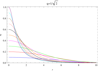
Figure 1: (Color online) The radial function of the scalar field, for a fixed value of the charge $q=q_{\mbox{\tiny{crit}}}=1/\sqrt{2}$ in units of $\sqrt{8\pi}m/M_{\mbox{\tiny{Pl}}}$, is plotted as a function of the radial coordinate $r$ for different values at the origin. The radial function decreases monotonically as the dimensionless radius increases.

In Fig. 2, the radial function $\phi$ is plotted for different initial values at the origin and for different values of the charge $q$. As expected $\phi$ decreases monotonically as the radius $r$ increases. Moreover, we see that for a fixed value of $r$ and of the central density, an increase of the boson charge corresponds to larger values of $\phi$.

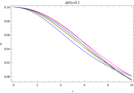
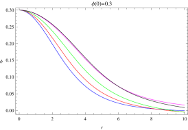
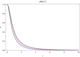
Figure 2: (Color online) The radial function $\phi$ is plotted as a function of $r$ (dimensionless) for selected values of the radial function at the origin and different values of the charge: $q=0$ (blue line), $q=0.5$ (red line), $q=0.65$ (green line), $q=0.7$ (magenta line), $q=1/\sqrt{2}$ (black line), in units of $\sqrt{8\pi}m/M_{\mbox{\tiny{Pl}}}$.

In Figs. 3 and 4 the metric function $e^{\lambda}=-g_{11}$ is plotted as a function of the dimensionless radius $r$ for different values of the radial function $\phi(r)$ at the origin and for a selected values of the charge $q$.

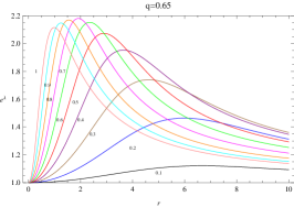
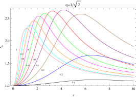
Figure 3: (Color online) The coefficient $e^{\lambda}$ of the metric is plotted as a function of $r$ (dimensionless) for different values of the radial function at the origin and for selected values of the charge $q$(in units of $\sqrt{8\pi}m/M_{\mbox{\tiny{Pl}}}$).

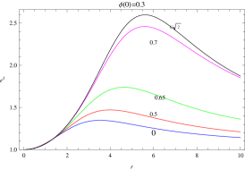
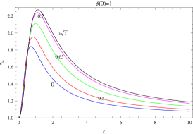
Figure 4: (Color online) The coefficient $e^{\lambda}=-g_{11}$ ($e^{\lambda(r)}$) of the metric is plotted as a function of $r$ (dimensionless) for fixed values of the radial function at the origin and for different values of the charge $q$(in units of $\sqrt{8\pi}m/M_{\mbox{\tiny{Pl}}}$).

.

In general, we observe that $e^{\lambda}$ reaches its maximum value at the value, say, $r_{\mbox{\tiny}{Max}}$ of the radial coordinate. Once the maximum is reached, the function decreases monotonically as $r$ increases and tends asymptotically to 1, in accordance with the imposed asymptotic behavior. For a fixed value of the charge, the value of $r_{\mbox{\tiny}{Max}}$ decreases as the central density increases.

Table 2 provides the maximum values of $e^{\lambda(r)}$ and the corresponding radial coordinate $r_{\mbox{\tiny}{Max}}$, for different values of the central density. In the case of a neutral configuration RR , $q=0$, the boson star radius is defined as the value $r_{\mbox{\tiny}{Max}}$ corresponding to the maximum value of $e^{\lambda(r)}=-g_{11}$. Then, the values of $r_{\mbox{\tiny}{Max}}$, listed in Table 2 can be assumed as good estimates of the radius of the corresponding charged configurations.

q	$\phi(0)$
	0.1		0.2		0.3		0.4		0.5
	$e^{\lambda_{\mbox{\tiny{Max}}}}$	$r_{\mbox{\tiny{Max}}}$	$e^{\lambda_{\mbox{\tiny{Max}}}}$	$r_{\mbox{\tiny{Max}}}$	$e^{\lambda_{\mbox{\tiny{Max}}}}$	$r_{\mbox{\tiny{Max}}}$	$e^{\lambda_{\mbox{\tiny{Max}}}}$	$r_{\mbox{\tiny{Max}}}$	$e^{\lambda_{\mbox{\tiny{Max}}}}$	$r_{\mbox{\tiny{Max}}}$
0	1.0984	6.4060	1.2328	4.7090	1.3471	3.5184	1.4528	2.7582	1.5482	2.2144
0.5	1.1179	6.8172	1.3132	5.2940	1.4705	3.9800	1.6094	3.1282	1.7234	2.512
0.65	1.1212	6.6753	1.4635	5.9912	1.7395	4.6225	1.9524	3.6451	2.0729	2.8975
0.7	1.1469	7.2189	1.8154	7.0841	2.4602	5.5813	2.5159	4.1125	2.5409	3.2099
$1/\sqrt{2}$	1.1323	6.8585	1.6764	6.5422	2.5981	5.6016	2.6873	4.1943	2.6637	3.2650
	$\phi(0)$
	0.6		0.7		0.8		0.9		1
0	1.6324	1.7964	1.7031	1.4561	1.7609	1.1707	1.8064	0.92659	1.8414	0.7175
0.5	1.8124	2.0394	1.8774	1.6600	1.9197	1.3430	1.9432	1.0722	1.9526	0.8383
0.65	2.1520	2.3519	2.1795	1.9132	2.1688	1.5471	2.1470	1.2464	2.1144	0.9895
0.7	2.5116	2.5649	2.4798	2.0919	2.3972	1.6925	2.3222	1.3706	2.2420	1.0939
$1/\sqrt{2}$	2.6123	2.6133	2.5519	2.1275	2.4469	1.7199	2.3420	1.3806	2.2745	1.1198

Table 2: The maximum values of $e^{\lambda(r)}=-g_{11}$ and the corresponding radial coordinate $r_{\mbox{\tiny}{Max}}$ for different values of the central density. For a fixed $\phi(0)$, an increase of the boson charge $q$ generates an increase of the maximum value of $e^{\lambda}$ and of the value of the radius $r_{\mbox{\tiny}{Max}}$.

Moreover, in Figs. 4, the coefficient $e^{\lambda}$ of the metric is plotted as a function of the radial coordinate $r$ for fixed values of the radial function at the origin and different values of the charge $q$. For a fixed $\phi(0)$, an increase in the maximum value of $g_{11}$ and of the value of $r_{\mbox{\tiny}{Max}}$, corresponds to an increase of the boson charge $q$. At a fixed value of $r$, the value of the coefficient $-g_{11}$ increases with an increase of the central density, reaching the maximum value at $\phi_{\mbox{\tiny{Max}}}(0)\simeq 0.3$.

IV.2 Mass, charge, radius and particle number

The masses $M$ and $M^{*}$ of the system, in units of $M_{\mbox{\tiny{Pl}}}^{2}/m$, and the particle number $N$, in units of $M_{\mbox{\tiny{Pl}}}^{2}/m^{2}$, are plotted in the Fig. 5 as functions of the central density $\phi(0)$, for different values of the boson charge $q$.

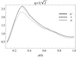
Figure 5: The charged boson star mass $M$ and mass $M^{*}$ in units of $M_{\mbox{\tiny{Pl}}}^{2}/m$ (solid line), and particle number $N$ in units of $M_{\mbox{\tiny{Pl}}}^{2}/m^{2}$ (dashed line) are plotted as functions of the central density $\phi(0)$ for different values of the charge $q$ (in units of $M_{\mbox{\tiny{Pl}}}/\sqrt{8\pi}m$). We note that in particular at the critical density $\phi(0)\approx 0.3$ for $q=1/\sqrt{2}$ it is $M^{*}>N$.

In Fig. 6, the masses $M$ and $M^{*}$ are plotted as functions of the scalar central density for selected values of the boson charge; we have indicated the difference $\Delta=M^{*}-M$ at a certain $\phi(0)$. This quantity clearly increases with the boson change $q$; as expected.

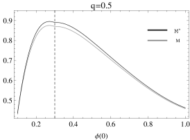
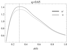
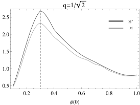
Figure 6: The mass $M$ (in units of $M_{\mbox{\tiny{Pl}}}^{2}/m$) and the mass $M^{*}$ are plotted as functions of the central density $\phi(0)$ and for different values of the boson charge $q$ (in units of $\sqrt{8\pi}m/M_{\mbox{\tiny{Pl}}}$).

Analogously to the case of white dwarf and neutron stars, a critical mass $M_{\mbox{\tiny{Max}}}$ and correspondingly a critical number $N_{\mbox{\tiny{Max}}}$ exist for a central density $\phi(0)_{\mbox{\tiny{Max}}}\simeq 0.3$, independently of the value of $q$. Configurations with $\phi(0)>\phi(0)_{\mbox{\tiny{Max}}}$ are gravitationally unstable, see e.g. Jetzer:1989av ; Jetzer:1989us ; Jetzer:1990wr ; Jetzer:1989fx ; Jetzer:1989qp ; Jetzer:1989vs ; Jetzer:1988af ; Jetzer:1988vr . In Table 3, the maximum values of the charged boson star mass $M_{\mbox{\tiny{Max}}}$, and the number of particles $N_{\mbox{\tiny{Max}}}$, and $\phi_{\mbox{\tiny{Max}}}$ are listed for selected values of $q$.

$q$	$M_{\mbox{\tiny{Max}}}$	$\phi(0)_{\mbox{\tiny{(Max,M)}}}$	$M^{*}_{\mbox{\tiny{Max}}}$	$\phi(0)_{\mbox{\tiny{(Max,$M^{*}$)}}}$	$N_{\mbox{\tiny{Max}}}$	$\phi(0)_{\mbox{\tiny{(Max,N)}}}$	$Q_{\mbox{\tiny{Max}}}$	$\phi(0)_{\mbox{\tiny{(Max,Q)}}}$	$R_{\mbox{\tiny{Max}}}$	$\phi(0)_{\mbox{\tiny{(Max,R)}}}$
0	0.62374	0.3	0.62374	0.3	0.641665	0.3	$\checkmark$	$\checkmark$	4.56589*	0.1*
0.50	0.87536	0.271041	0.895504	0.271444	0.902576	0.271361	0.448485	0.3	4.79634*	0.1*
0.65	1.33207	0.325797	1.4133	0.32305	1.402170	0.326816	0.90818	0.318766	4.63946	0.091957
0.70	2.31504	0.282575	2.63956	0.291404	2.63120	0.284047	1.84184	0.284047	4.74968*	0.1*
$1/\sqrt{2}$	2.33016	0.3	2.67951	0.3	2.64329	0.3	1.86909	0.3	$5.14269$	$0.158228$

Table 3: The maximum values of the boson star mass $M_{\mbox{\tiny{Max}}}$ and $M^{*}_{\mbox{\tiny{Max}}}$ (in units of $M_{\mbox{\tiny{Pl}}}^{2}/m$) and of the number of particles $N_{\mbox{\tiny{Max}}}$ (in units of $M_{\mbox{\tiny{Pl}}}^{2}/m^{2}$), the charge $Q_{\mbox{\tiny{Max}}}$ (in units of $\sqrt{8\pi}M_{\mbox{\tiny{Pl}}}/m$) as functions of $\phi(0)$, and the corresponding central density values $\phi(0)_{\mbox{\tiny{(Max,M)}}}$ for the mass $M_{\mbox{\tiny{Max}}}$, $\phi(0)_{\mbox{\tiny{(Max,N)}}}$ for particle number $N_{\mbox{\tiny{Max}}}$, $\phi(0)_{\mbox{\tiny{(Max,Q)}}}$ for the total charge $Q_{\mbox{\tiny{Max}}}$ are listed for different $q$. The entries with a star $(*)$ do not correspond to maximum values but to the initial points of the numerical integration. (See Fig. 7)

Comparing the plots at different charge values we can see that the presence of charge does not change the behavior qualitatively. However, to an increase of the boson charge values corresponds an increase of $M_{\mbox{\tiny{Max}}}$, $M^{*}_{\mbox{\tiny{Max}}}$ and $N_{\mbox{\tiny{Max}}}$, and an increase of the difference $(N_{\mbox{\tiny{Max}}}-M_{\mbox{\tiny{Max}}})$ between the maximum number of particles and the mass at a fixed central density. The critical central density value is $\phi(0)_{\mbox{\tiny{Max}}}\simeq 0.3$. This value seems to be independent of the charge values $q$ (see also Jetzer:1990xa ).

The radius $R$, the total charge $Q$, and the mass $M$ are plotted (in units of $1/m$, $\sqrt{8\pi}M_{\mbox{\tiny{Pl}}}/m$, and $M_{\mbox{\tiny{Pl}}}^{2}/m$, respectively) in Figs. 7–8 as functions of the central density $\phi(0)$, for different values of the charge $q$. We see that the radius, for a fixed central density, increases as the charge increases (see Fig. 7 and Table 3).

In Table 3 the maximum values of the total charge $Q_{\mbox{\tiny{Max}}}$, for $\phi_{\mbox{\tiny{Max}}}(0)\simeq 0.3$ and for different $q$ are listed. For fixed values of the charge $q$, the total charge increases with an increase of the central density until it reaches a maximum value for some density $\phi(0)_{\mbox{\tiny{Max}}}$. Then, the value of $Q$ decreases monotonically as $\phi(0)$ increases. In this way, it is possible to introduce the concept of a maximum charge $Q_{\mbox{\tiny{Max}}}$ for charged boson stars.

In Fig. 7, the charge $Q$ is plotted as a function of the central density $\phi(0)$ for different values of the charge $q$. For fixed values of the charge $q$, the total charge increases with an increase of the central density until it reaches a maximum value for some density $\phi(0)_{\mbox{\tiny{Max}}}$. Then, the value of $Q$ decreases monotonically as $\phi(0)$ increases. In this way, it is possible to introduce the concept of a critical charge $Q_{\mbox{\tiny{Max}}}$ for charged boson stars. In Table 3 the maximum values of the total charge $Q_{\mbox{\tiny{Max}}}$, for $\phi_{\mbox{\tiny{Max}}}(0)\simeq 0.3$ and for different values of $q$ are listed. Let us note that for a fixed central density, to an increase of the boson charge $q$ corresponds an increase of the maximum $Q_{\mbox{\tiny{Max}}}$ (see Fig. 7 and Table 3).

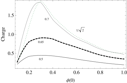
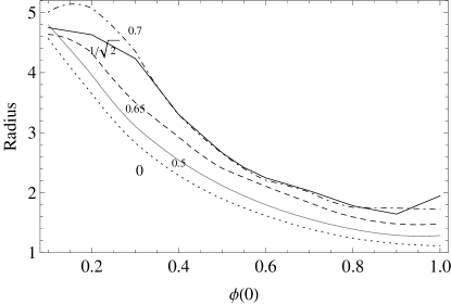
Figure 7: This graphic shows the total charge $Q$ (in units of $\sqrt{8\pi}M_{\mbox{\tiny{Pl}}}/m$) and the radius $R$ (in units of $1/m$) as functions of the central density $\phi(0)$, for different values of the boson charge $q$ (in units $\sqrt{8\pi}m/M_{\mbox{\tiny{Pl}}}$).

Fig. 8 depicts the total charge $Q$ (in units of $\sqrt{8\pi}M_{\mbox{\tiny{Pl}}}/m$), the radius $R$ (in units of $1/m$), and the mass $M$ (in units of $M_{\mbox{\tiny{Pl}}}^{2}/m$), as functions of the central density $\phi(0)$ and for different values of the boson charge $q$ (in $\sqrt{8\pi}m/M_{\mbox{\tiny{Pl}}}$).

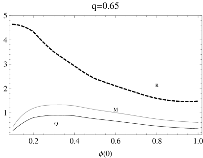
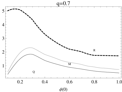
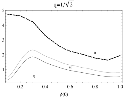
Figure 8: The total charge $Q$ (in units of $\sqrt{8\pi}M_{\mbox{\tiny{Pl}}}/m$), the radius $R$ (in units of $1/m$), and the mass $M$ (in units of $M_{\mbox{\tiny{Pl}}}^{2}/m$) are plotted as functions of the central density $\phi(0)$ and for different values of the boson charge $q$ (in units of $\sqrt{8\pi}m/M_{\mbox{\tiny{Pl}}}$).

Note that, for a fixed value of the charge $q$, the mass, the radius and the charge are always positive and to an increase (decrease) of the total charge there always corresponds an increase (decrease) of the total mass (and total particle number). Both quantities increase as the central density increases and they reach a maximum value for the same density $\phi(0)_{\mbox{\tiny{Max}}}\simeq 0.3$ (see also Table 3). Once the maximum is reached, both quantities decrease monotonically as $\phi(0)$ increases.

In Figs. 9 we show the ratios $R/N$, $R/M$ and $R/M^{*}$, $M/N$ and $M^{*}/N$ in units of $m/M^{2}_{\mbox{\tiny{Pl}}}$, $1/M^{2}_{\mbox{\tiny{Pl}}}$ and $m$, respectively, as functions of the central density, and for different values of the boson charge $q$.

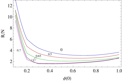
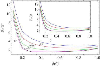
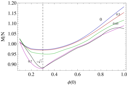
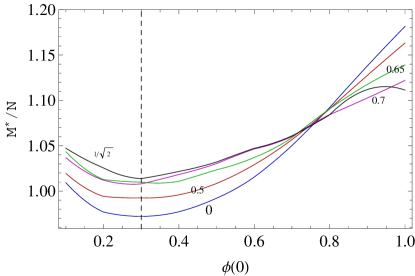
Figure 9: (Color online) The ratios $R/N$ (upper left plot), $R/M^{*}$ (upper right), $M/N$ (bottom right) and $M^{*}/N$ (bottom left) in units of $m/M^{2}_{\mbox{\tiny{Pl}}}$, $1/M^{2}_{\mbox{\tiny{Pl}}}$, and $m$, respectively, are plotted as functions of the central density, and for different values of the boson charge $q$ (in $\sqrt{8\pi}m/M_{\mbox{\tiny{Pl}}}$). Dashed line is $\phi(0)=0.3$.

.

For fixed values of the charge $q$, the ratio $R/N$, the ratio $R/M$, and $M/N$ decrease as the central density increases, until they reach a minimum value $\phi(0)_{\mbox{\tiny{(min,R/N)}}}$, $\phi(0)_{\mbox{\tiny{(min,R/M)}}}$, $\phi(0)_{\mbox{\tiny{(min,M/N)}}}$, respectively. After the minimum is reached, all ratios increase monotonically as the central density increases.

In Table 4, the minimum values of $R/N$, $M/N$ and $R/M$, $M^{*}/N$ and $R/M^{*}$ and the value of $\phi_{\mbox{\tiny{min}}}$, are given for different values of $q$.

$q$	$\frac{R(\phi(0))}{M(\phi(0))}$	$\phi(0)_{\mbox{\tiny{(min,R/M)}}}$	$\frac{R(\phi(0))}{M^{*}(\phi(0))}$	$\phi(0)_{\mbox{\tiny{(min,$R/M^{*}$)}}}$	$\frac{M(\phi(0))}{N(\phi(0))}$	$\phi(0)_{\mbox{\tiny{(min,M/N)}}}$	$\frac{M^{*}(\phi(0))}{N(\phi(0))}$	$\phi(0)_{\mbox{\tiny{(min,$M^{*}/N$)}}}$	$\frac{R(\phi(0))}{N(\phi(0))}$	$\phi(0)_{\mbox{\tiny{(min,R/N)}}}$
0	2.87985	0.793811	2.87985	0.793811	0.972071	0.298102	0.972071	0.298102	3.07529	0.691860
0.50	2.47116	0.742725	2.43821	0.735351	0.969991	0.291616	0.992362	0.282309	2.56920	0.648890
0.65	2.08637	0.617825	2.00041	0.592344	0.949828	0.334285	1.00875	0.342184	2.06194	0.535094
0.70	1.76082	0.541418	1.63117	0.455206	0.879342	0.289220	1.00752	0.278012	1.66369	0.340757
$1/\sqrt{2}$	1.68120	0.499717	1.53638	0.446416	0.881540	0.300000	1.0137	0.300000	1.57425	0.424978

Table 4: The minimum values of the ratios $R/M$ and $R/M^{*}$ (in units of $1/M_{\mbox{\tiny{Pl}}}^{2}$), $M/N$ and $M^{*}/N$ (in units of $m$) and $R/N$ (in units of $m/M_{\mbox{\tiny{Pl}}}^{2}$) as functions of $\phi(0)$ and for different values of $q$. We note that to an increase of $q$ corresponds a decrease of the minima of $R/M$, $R/M^{*}$, $M/N$, and $R/N$. Viceversa the $M^{*}/N$ increases with $q$.

Furthermore, an increase of the boson charge values corresponds a decrease of the minima of the ratios $R/N$ and $R/M$, and of the corresponding $\phi_{\mbox{\tiny{min}}}$. For a fixed value of the central density $\phi(0)$, to a decrease of the boson charge $q$ corresponds an increase of $R/N$, $R/M$ and $R/M^{*}$. These ratios decrease as the particle repulsion increases, leading to a minimum value for a given central density. The ratio $M/N$ and $M^{*}/N$ decrease with an increase of the central density until it reaches a minimum value, and then it increases as $\phi(0)$ increases. The minimum values of $M/N$ decrease as the charge $q$ increases. On the other side, from Table 4, we note that the minimum values of $M^{*}/N$ increases as the charge $q$ increases. This can also be noted in Figs. 9: $M^{*}/N$ increases with $q$ until the central density reaches a point $\phi(0)\approx 0.75$, at which the lines $M^{*}/N$ at different charges match and then $M^{*}/N$ turns out to be a decreasing function of $q$. It is clear that the quantity $M/N$ is an indication of the binding energy per particle, $B/N=1-M/N$, in the units we are using. So $M/N>1$ indicates negative binding energies (bound particles) while $M/N<1$ indicates unbound particles, in principle. It can be seen from the lower left panel of Fig. 9 how the misinterpretation of the mass $M$ as the mass of the system would in principle lead to the conclusion that most of the configurations have positive binding energy, since $M/N<1$. Instead, the lower right panel of Fig. 9 shows that indeed most of the configurations have $M^{*}/N>1$ and have therefore negative binding. However, it can be also seen from this figure that indeed there are configurations for which despite being in the stable branch, $\phi(0)\leq 0.3$, their binding energy is positive for some values of the central density. In contrast, the configurations at the critical point, $\phi(0)\approx 0.3$, and over it, show negative binding energies; this means that objects apparently bound can be unstable against small perturbations, in full analogy with what observed in the mass-radius relation of neutron stars. For a discussion on this issue see, for instance, Kleihaus:2009kr ; Kleihaus:2011sx .

Figs. 10 illustrate the behavior of the ratios $Q/M$, $Q/M^{*}$ and $Q/R$ in units of $\sqrt{8\pi}/M_{\mbox{\tiny{Pl}}}$ and $\sqrt{8\pi}M_{\mbox{\tiny{Pl}}}$, respectively, as functions of the central density for different values of the boson charge $q$. The maximum values of the charge-to-mass ratio satisfy the inequality $Q/M>Q/M^{*}$ since $M<M^{*}$ as shown in Fig. 6. We also note that the inequality $Q/M^{*}<q/m$ is satisfied for all charges $q$, in particular $Q/M^{*}$ never reaches the critical value $q_{crit}/m$; a consequence of the non-zero gravitational binding.

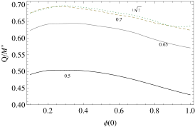
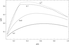
Figure 10: The ratios $Q/M$ (left) and $Q/M^{*}$ (center) in units of $\sqrt{8\pi}/M_{\mbox{\tiny{Pl}}}$, and $Q/R$ (right), in units of $\sqrt{8\pi}M_{\mbox{\tiny{Pl}}}$, as functions of the central density, for different values of the boson charge $q$ (in $\sqrt{8\pi}m/M_{\mbox{\tiny{Pl}}}$).

To an increase of the central density corresponds an increase of the $Q/M$ ($Q/M^{*}$) ratio, until a maximum value is reached. As the boson charge $q$ increases, the values of the maximum of $Q/M$ ($Q/M^{*}$) increase. Table 5 provides the maximum value of the ratios $Q/M$, $Q/M^{*}$ and $Q/R$ as functions of the central density and for different values of the boson charge $q$.

$q$	$\frac{Q}{M}(\phi(0))$	$\phi(0)_{\mbox{\tiny{(Max,Q/M)}}}$	$\frac{Q}{M^{*}}(\phi(0))$	$\phi(0)_{\mbox{\tiny{(Max,$Q/M^{*}$)}}}$	$\frac{Q}{R}(\phi(0)$	$\phi(0)_{\mbox{\tiny{(Max,Q/R)}}}$
0.50	0.515469	0.291645	0.503848	0.282348	0.194576	0.648848
0.65	0.684291	0.333835	0.644347	0.34207	0.315191	0.534444
0.70	0.796011	0.289606	0.694768	0.278139	0.420745	0.340640
$1/\sqrt{2}$	0.802127	0.300000	0.697547	0.300000	0.449011	0.422762

Table 5: The maximum value of the ratios $Q/M$, $Q/M^{*}$, and $Q/R$, in units of $\sqrt{8\pi}/M_{\mbox{\tiny{Pl}}}$ and $\sqrt{8\pi}M_{\mbox{\tiny{Pl}}}$ respectively, as functions of the central density and for different values of the boson charge $q$ (in $\sqrt{8\pi}m/M_{\mbox{\tiny{Pl}}}$).

The behavior of the total mass $M$ and $M^{*}$, particle number $N$ and charge $Q$ as functions of the configuration radius $R$ is also shown in Figs. 11, for different values of the charge $q$.

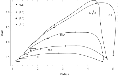
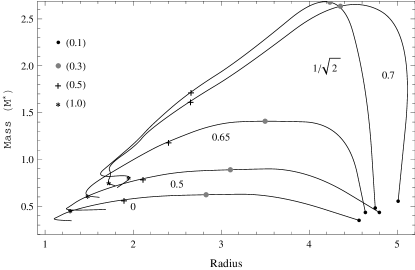
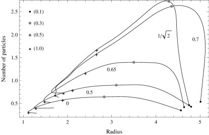
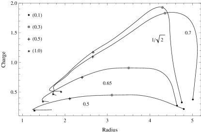
Figure 11: The mass $M$ and $M^{*}$, in units of $M_{\mbox{\tiny{Pl}}}^{2}/m$, the particle number $N$, in units of $M_{\mbox{\tiny{Pl}}}^{2}/m^{2}$, and the charge $Q$, in units of $\sqrt{8\pi}M_{\mbox{\tiny{Pl}}}/m$, as functions of the radius $R$ calculated at a fixed central value $\phi(0)$, in units of $1/m$, for different values of the charge $q$, in units of $\sqrt{8\pi}m/M_{\mbox{\tiny{Pl}}}$. The central density values $\phi(0)$ are represented by markers on the curves and numbers in brackets.

We can note that, for a fixed values of the charge $q$, the mass, the particle number and the charge, increase as the radius $R$ increases, until a maximum value is reached for the same $R_{\mbox{\tiny{Max}}}$. Then all these quantities decrease rapidly as $R$ increases. This means that the concept of “critical radius” $R_{\mbox{\tiny{Max}}}$, together with a critical mass and a critical particle number, for a charged boson star can be introduced. The plots also indicate that the presence of a charge $q$ does not change the qualitative behavior of the quantities. However, the values of $M_{\mbox{\tiny{Max}}}$ and $N_{\mbox{\tiny{Max}}}$, and of the corresponding values of $R_{\mbox{\tiny{Max}}}$, are proportional to the value of $q$. Configurations are allowed only within a finite interval of the radius $R$. The values of the minimum and maximum radii are also proportional to the value of the boson charge $q$. The critical central density $\phi(0)\simeq 0.3$ represents a critical point of the curves. Configurations for $\phi(0)>0.3$, are expected to be unstable, see Jetzer:1989av ; Jetzer:1990wr . It is interesting to notice that for small values of the radius, there is a particular range at which for a specific radius value there exist two possible configurations with different masses and particle numbers. This behavior has also been found in the case of neutral configurations and is associated with the stability properties of the system.

Finally, we illustrate the behavior of the physical quantities for a fixed value of the charge $q$ in Fig. 12.

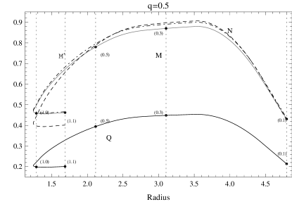
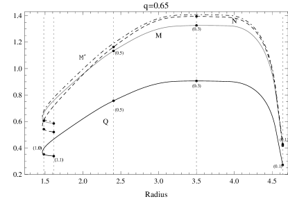
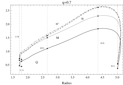
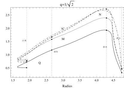
Figure 12: The total charge $Q$ in $\sqrt{8\pi}M_{\mbox{\tiny{Pl}}}/m$ (black curve), the total mass $M$ (gray curve) and $M^{*}$ (dotted–dashed curve) in $M_{\mbox{\tiny{Pl}}}^{2}/m$, and the particle number $N$ (dashed curve) in units of $M_{\mbox{\tiny{Pl}}}^{2}/m^{2}$ are plotted as functions of the radius $R$ (in units of $1/m$) for different values of the charge $q$ (in units of $\sqrt{8\pi}m/M_{\mbox{\tiny{Pl}}}$). Dotted lines represent the curves $\phi(0)=const.$; the central density values are designed by points of the curves and numbers in brackets.

Figures 13 show the charge-to-mass ratio as a function of the radius of the configuration evaluated at different central densities. At the central density $\phi(0)\simeq 0.3$ there exists a critical point on the curve. To lower central densities correspond configurations with larger radius. The ratio $Q/(RM)$ and $Q/(RM^{*})$ and increases as $\phi(0)$ increases.

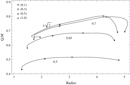
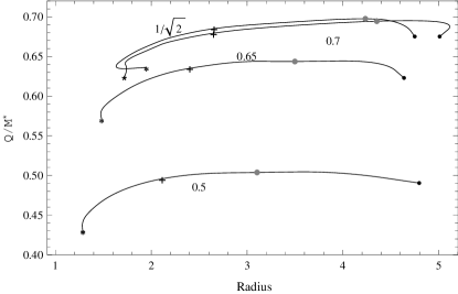
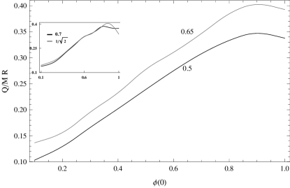
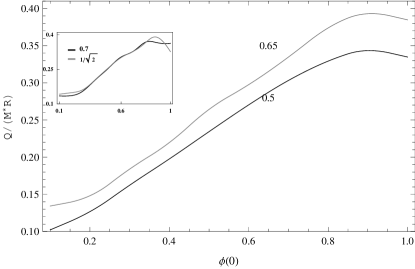
Figure 13: Upper plot: The charge-to-mass ratio $Q/M$ and $Q/M^{*}$ in units of $\sqrt{8\pi}/M_{\mbox{\tiny{Pl}}}$ is plotted in terms of the radius $R$ (in units of $1/m$) for different values of the charge $q$ (in units of $\sqrt{8\pi}m/M_{\mbox{\tiny{Pl}}}$). The central density values $\phi(0)$ are represented by markers on the curves and numbers in brackets. Bottom plot: The ratio $Q/(MR)$ and $Q/(M^{*}R)$ in units of $m\sqrt{8\pi}/M_{\mbox{\tiny{Pl}}}$ is plotted as a function of the central density $\phi(0)$ for different values of the charge (in units of $\sqrt{8\pi}m/M_{\mbox{\tiny{Pl}}}$): $q=0.5$ (black curve) and $q=0.65$ (gray curve). The inset plot shows the curves $q=0.7$ (black curve) and $q=1/\sqrt{2}$ (gray curve).

V Conclusions

In this work we studied spherically symmetric charged boson stars. We have solved numerically the Einstein-Maxwell system of equations coupled to the general relativistic Klein-Gordon equations of a complex scalar field with a local $U(1)$ symmetry.

As in the case of neutral boson stars and previous works on charged configurations, we found that it is possible to introduce the concepts of critical mass $M_{\mbox{\tiny{Max}}}$ and critical number $N_{\mbox{\tiny{Max}}}$. It turns out that the explicit value of these quantities increases as the value of the boson charge $q$ increases. In previous works Jetzer:1990wr ; Jetzer:1989av , it was shown that charged configurations are possible for $q<q_{\mbox{\tiny{crit}}}\equiv\sqrt{1/2}$ (in units of $\sqrt{8\pi}m/M_{\mbox{\tiny{Pl}}}$). We performed a more detailed analysis and determined that bounded charged configurations of self-gravitating bosons are possible with a particle charge $q=q_{\mbox{\tiny{crit}}}$, and even for higher values localized solutions can exist.

We compared and contrasted both from the qualitative and quantitative point of view the function $M$ given by Eq. (31), often misinterpreted as the mass of a charged system, with the actual mass $M^{*}$, related to $M$ by Eq. (33), which allows a correct matching of the interior solution at the surface with the exterior Reissner-Nordström spacetime.

By means of numerical integrations it is possible to show that for $q>q_{\mbox{\tiny{crit}}}$ solutions satisfying the given initial conditions, without nodes are possible only for small values of the central density smaller than the critical value $\phi(0)\approx 0.3$ (see e.g. Fig. 14).

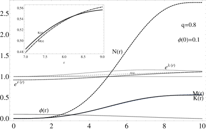
Figure 14: The radial function of the scalar field $\phi(r)$ (gray curve) for the charge $q=0.8$ in units of $\sqrt{8\pi}m/M_{\mbox{\tiny{Pl}}}$, $\omega=1.10893$ and for central density $\phi(0)=0.1$, function of the radial coordinate $r$. Dotted curve is $e^{\nu(r)}$, black curve is $e^{\lambda(r)}$, dashed curve is $C(r)$. Dashed thick curve is $N(r)$. Inside plot is a enlarged view of the curve $M(r)$ (dotted-dashed curve), and $K(r)$ (black thick curve) where $R=\int^{\infty}_{0}K^{\prime}(r)dr$. It is $e^{\lambda}_{\mbox{\tiny{Max}}}=1.15874$ in $r_{\mbox{\tiny{Max}}}=7.18885$. Moreover the configuration mass $M=0.570768$ and $M^{*}=0.590706$ measured in units of $M_{\mbox{\tiny{Pl}}}^{2}/m$. The particle number $N=0.558146$ , in units of $M_{\mbox{\tiny{Pl}}}^{2}/m^{2}$, and the radius $R=4.95246$ and the total charge $Q=qN=0.446517$ in units of $1/m$ and $\sqrt{8\pi}M_{\mbox{\tiny{Pl}}}/m$, respectively. Moreover, it is $Q/R=0.0901607$, $R/N=8.87305$, $R/M=8.67684$, $R/M^{*}=8.38397$, $M/N=1.02261$, $M^{*}/N=1.05833$, $Q/M=0.78231$, $Q/M^{*}=0.755905$. Here $R/M$ and $R/M^{*}$ are in units of $1/M_{\mbox{\tiny{Pl}}}^{2}$, $M/N$ and $M^{*}/N$ in units of $m$ and $R/N$ in units of $m/M_{\mbox{\tiny{Pl}}}^{2}$, $Q/M$, $Q/M^{*}$, and $Q/R$, in units of $\sqrt{8\pi}/M_{\mbox{\tiny{Pl}}}$ and $\sqrt{8\pi}M_{\mbox{\tiny{Pl}}}$, respectively

On the other hand, for $q>q_{\mbox{\tiny{crit}}}$ and higher central densities the boundary conditions for zero-node solutions at the origin are not satisfied and only bounded configurations with one or more nodes could be possible.

We established that the critical central density value corresponding to $M_{\mbox{\tiny{Max}}}$ ($M^{*}_{\mbox{\tiny{Max}}}$) and $N_{\mbox{\tiny{Max}}}$ is $\phi(0)_{\mbox{\tiny{Max}}}\simeq 0.3$, independently of the boson charge $q$. The critical total mass and number of particles increase as the electromagnetic repulsion increases Jetzer:1990wr (see Hod:2010zk ; Madsen:2008vq , and also Eilers:2013lla ; Hartmann:2012gw ; Lieb-Pale12 , for a recent discussion on the charge-radius relation for compact objects).

The total charge of the star increases with an increase of the value of the central density until it reaches a maximum value at $\phi(0)=\phi(0)_{\mbox{\tiny{Max}}}\simeq 0.3$. As $\phi(0)$ continues to increase, the charge $Q$ decreases monotonically. In this manner, the concept of a critical charge $Q_{\mbox{\tiny{Max}}}$ for charged boson stars can be introduced in close analogy to the concept of $N_{\mbox{\tiny{Max}}}$. In this respect, the value $\phi(0)\simeq 0.3$ plays the role of a point of maximum of the electromagnetic repulsion (as a function of the central density).

In order to have a better understanding of these systems for $\phi\simeq\phi(0)_{\mbox{\tiny{Max}}}$, we studied the behavior of $\phi$ and $g_{11}$ as functions of $\phi(0)$ and the radial coordinate $r$. The density $\phi$ increases with larger values of $q$, at fixed $r$ and fixed central density. For a fixed value of the boson charge, $g_{11}$ reaches a maximum value corresponding to a value $r_{\mbox{\tiny}{Max}}$ of the radial coordinate. After this maximum is reached, it decreases monotonically with an arbitrary increase of $r$. The maximum value of $g_{11}$ depends on the value of the central density and of the coupling constant $q$. However, this maximum is bound and reaches its highest value for $\phi_{\mbox{\tiny{Max}}}(0)\simeq 0.3$.

The radius $R$ and the ratios $Q/M$, $M/N$, $R/M$, $Q/M^{*}$, $M^{*}/N$, $R/M^{*}$, $R/N$, $Q/R$ were also studied as functions of the central density. To the central density value $\phi(0)\simeq 0.3$ corresponds the maxima of the charge $Q$, the mass $M$ $(M^{*})$, the particle number $N$, and of the ratio $Q/M$ ($Q/M^{*}$). On the other hand, $\phi(0)\simeq 0.3$ corresponds to the minima of $M/N$, $R/N$ and $R/M$ as well as $M^{*}/N$ and $R/M^{*}$.

The effects of the introduction of the mass definition $M^{*}$ are evident in the analysis of the behavior of $Q/M^{*}$ and $M^{*}/N$ with respect to $Q/M$ and $M/N$: we note that the minimum value of $M^{*}/N$ increases as the charge $q$ increases while $M/N$ decreases always with $q$. In particular $M^{*}/N$ increases with $q$ until the central density reaches a point $\phi(0)\approx 0.75$, at which the lines $M^{*}/N$ at different charges match and then $M^{*}/N$ turns out to be a decreasing function of $q$.

The maximum values of the charge-to-mass ratio satisfy the inequality $Q/M^{*}<q/m$ for all charges $q$, in particular $Q/M^{*}$ never reaches the critical value $q_{crit}/m$. The contrary conclusion would be reached if the misinterpreted mass $M$ were used since the inequality $Q/M>Q/M^{*}$ is satisfied, i.e. the charge-to-mass ratio $Q/M$ indeed attain values larger than $q_{crit}/m$ (see e.g. Fig. 10). To summarize, we found that all the relevant quantities that characterize charged boson stars behave in accordance with the physical expectations. Bounded configurations are possible only within an interval of specific values for the bosonic charge and the central density.

Appendix A Neutral boson stars

In this Appendix we shall focus on electrically neutral configurations exploring in particular their global proprieties: mass, radius and total particle numbers. Neutral boson stars are gravitationally bound, spherically symmetric, equilibrium configurations of complex scalar fields $\phi$ RR . It is possible to analyze their interaction by considering the field equations describing a system of free particles in a curved space–time with a metric determined by the particles themselves.

The Lagrangian density of the gravitationally coupled complex scalar field $\phi$ reads

$$\mathcal{L}=-\left(g^{\mu\nu}\partial_{\mu}\ \phi\partial_{\nu}\phi^{*}-m^{2}\phi\phi^{*}\right)$$ (42)

where $m$ is the boson mass, $\phi^{*}$ is the complex conjugate field (see, for example, RR ; Fulling ; BD ). This Lagrangian is invariant under global phase transformation $\phi\rightarrow\exp\left(i\theta\right)\phi$ where $\theta$ is a real constant that implies the conservation of the total particle number $N$.

Using the variational principle with the Lagrangian (42), we find the following Einstein coupled equations

$$G_{\mu\nu}\equiv R_{\mu\nu}-\frac{1}{2}g_{\mu\nu}R=8\pi G_{\mbox{\tiny{N}}}T_{\mu\nu}(\phi),$$ (43)

with the following Klein-Gordon equations

$$g^{\mu\nu}\nabla_{\mu}\nabla_{\nu}\phi+m^{2}\phi = 0,$$ (44)

$$g^{\mu\nu}\nabla_{\mu}\nabla_{\nu}\phi^{*}+m^{2}\phi^{*} = 0.$$ (45)

for the field $\phi$ and its complex conjugate $\phi^{*}$.

The symmetric energy-momentum tensor is

$$T_{\mu\nu}=2\left(|g|\right)^{-1/2}\left(\frac{\partial}{\partial x^{\alpha}}\frac{\partial\left(\sqrt{-g}\right)\mathcal{L}}{\partial\left(g^{\mu\nu}/\partial x^{\alpha}\right)}-\frac{\partial\left(\sqrt{-g}\right)\mathcal{L}}{\partial g^{\mu\nu}}\right),$$ (46)

and the current vector is

$$J^{\mu}=\imath\left\{\left[\frac{\partial\mathcal{L}}{\partial\left(\partial_{\mu}\phi^{*}\right)}\phi^{*}\right]-\left[\frac{\partial\mathcal{L}}{\partial\left(\partial_{\mu}\phi\right)}\phi\right]\right\}\ .$$ (47)

The explicit form of Eq. (44)

$$\frac{1}{\sqrt{|g|}}\partial_{i}\left[g^{ij}\sqrt{|g|}\partial_{k}\phi\right]+g^{00}\partial_{0}^{2}\phi+m^{2}\phi=0\ ,$$ (48)

can be solved by using separation of variables

$$\phi\left(r,\theta,\varphi,t\right)=R(r)Y_{l}^{m}\left(\theta,\varphi\right)e^{-\imath\omega t},$$ (49)

where $Y_{l}^{m}\left(\theta,\varphi\right)$ is the spherical harmonic. Equation (49) and its complex conjugate describe a spherically symmetric bound state of scalar fields with positive or negative frequency $\omega$, respectively. It ensures that the boson star space–time remains static.

In the case of spherical symmetry, we use as before the general line element

$$ds^{2}=e^{\nu}dt^{2}-e^{\lambda}dr^{2}-r^{2}\left(d\vartheta^{2}+\sin\vartheta^{2}d\varphi^{2}\right)\ ,$$ (50)

where $\lambda=\lambda(r)$ and $\nu=\nu(r)$.

Thus, there are only three unknown functions of the radial coordinate $r$ to be determined, the metric function $\nu,\lambda$, and the radial component $R$ of the Klein–Gordon field. From Eq. (48) we infer the radial Klein–Gordon equation

$$R^{\prime\prime}(r)+\left(\frac{2}{r}-\frac{\lambda^{\prime}(r)}{2}+\frac{\nu^{\prime}(r)}{2}\right)R^{\prime}(r)+e^{\lambda(r)}\left(-m^{2}+e^{-\nu(r)}\omega^{2}\right)R(r)=0,$$ (51)

where the prime $(^{\prime})$ denotes the differentiation with respect to $r$.

The energy momentum tensor components are (see RR )

$$T^{\phantom{\ }0}_{0} = \frac{1}{2}\left\{\left[e^{-\nu}\omega^{2}+m^{2}\right]R_{01}^{2}+e^{-\lambda}R_{01}^{{}^{\prime}2}\right\},$$ (52)

$$T^{\phantom{\ }1}_{1} = -\frac{1}{2}\left\{\left[e^{-\nu}\omega^{2}-m^{2}\right]R_{01}^{2}+e^{-\lambda}R_{01}^{{}^{\prime}2}\right\},$$ (53)

$$T^{\phantom{\ }2}_{2} = {T}^{\phantom{\ }3}_{3}=-\frac{1}{2}\left\{\left[e^{-\nu}\omega^{2}-m^{2}\right]R_{01}^{2}-e^{-\lambda}R_{01}^{{}^{\prime}2}\right\},$$ (54)

$$T^{\phantom{\ }i}_{0} = 0$$ (55)

From the expressions (52,53) and from the Einstein equation (43) we finally obtain the following two independent equations

$$\lambda^{\prime} = \frac{1}{r}\left(1-e^{\lambda}\right)+8\pi Gre^{-\nu}\left[R^{2}e^{\lambda}\left(\omega^{2}+m^{2}e^{\nu}\right)+R^{\prime 2}{e^{\nu}}\right],$$ (56)

$$\nu^{\prime} = -\frac{1}{r}\left(1-e^{\lambda}\right)+8\pi Gre^{-\nu}\left[R^{2}e^{\lambda}\left(\omega^{2}-m^{2}e^{\nu}\right)+R^{\prime 2}{e^{\nu}}\right],$$ (57)

for the metric fields $\lambda$ and $\nu$, respectively.

To integrate numerically these equations it is convenient to make the following rescaling of variables:

$$r\rightarrow\hat{r}/m,\quad\sigma(r)\equiv R(r)/\sqrt{8\pi G_{N}},\quad\omega\rightarrow\omega m\ .$$ (58)

Thus, we finally obtain from Eqs. (51) and (56, 57) the following equations

$$R^{\prime\prime} = e^{\lambda}R-\omega^{2}e^{\lambda-\nu}R+R^{\prime}\left(-\frac{1}{r}-\frac{e^{\lambda}}{r}+e^{\lambda}rR^{2}\right)$$ (59)

$$\lambda^{\prime} = \frac{1}{r}\left(1-e^{\lambda}\right)+re^{-\nu}\left[R^{2}e^{\lambda}\left(\omega^{2}+e^{\nu}\right)+R^{\prime 2}{e^{\nu}}\right],$$ (60)

$$\nu^{\prime} = -\frac{1}{r}\left(1-e^{\lambda}\right)+re^{-\nu}\left[R^{2}e^{\lambda}\left(\omega^{2}-e^{\nu}\right)+R^{\prime 2}{e^{\nu}}\right],$$ (61)

for the radial part of the scalar field $R$ and the metric coefficients $\lambda$ and $\nu$ in the dimensionless variable $\hat{r}$.

The initial and boundary conditions we impose are

$$R(\infty)=0,\quad R^{\prime}(\infty)=0,\quad\mbox{and}\quad R(0)=\mbox{constant},\quad R^{\prime}(0)=0.$$ (62)

in order to have a localized particle distribution and

$$\lambda(0) = 0,$$ (63)

$$\nu(\infty) = 0,$$ (64)

to get asymptotically the ordinary Minkowski metric (63), and to satisfy the regularity condition (64).

We calculate the mass of system as

$$M=4\pi\int_{0}^{\infty}\rho r^{2}dr,$$ (65)

where the density $\rho$, given by $T_{0}^{0}$, is

$$\rho=\frac{1}{2}\left[R^{2}\left(1+\omega^{2}e^{-\nu}\right)+e^{-\lambda}R^{\prime 2}\right].$$ (66)

The particle number is determined by the following normalization condition

$$N=\int_{0}^{\infty}\left\langle J^{0}\right\rangle\left(-g\right)^{1/2}d^{3}x.$$ (67)

which, using Eq. (47), becomes

$$N=\int_{0}^{\infty}r^{2}\omega e^{(\lambda-\nu)/2}R^{2}dr.$$ (68)

The mass $M$ is measured in units of $M_{\mbox{\tiny{Pl}}}^{2}/m$, the particle number $N$ in units of $M_{\mbox{\tiny{Pl}}}^{2}/m^{2}$, $\omega$ in units of $mc^{2}$ and the radius of the configuration is in units of $\hbar/(mc)$.

In the numerical analysis we obtain a maximum value of $g_{11}$ from which we determine the “effective radius” $R_{\mbox{\tiny{eff}}}$ of the distribution as the radius, $r_{g_{11}^{\mbox{\tiny{Max}}}}$, corresponding to the maximum of $g_{11}$ RR ; Schunck:2003kk . We carried out a numerical integration for different values of the radial function $R$ at the origin. We give some numerical values in Table 6.

$R\left(0\right)$	$\omega$ $\left(mc^{2}\right)$	$g^{\mbox{\tiny{Max}}}_{11}$	$r_{g_{11}^{\mbox{\tiny{Max}}}}$$(\hbar/mc)$	$g^{\mbox{\tiny{min}}}_{00}$	$g_{00}\left(r_{\mbox{\tiny{Max}}}\right)$	N $(m^{-2}M_{Pl}^{2})$	M $(M_{Pl}^{-2}/m)$
0.10	1.0000	1.10572	6.73590	0.860104	0.959895	0.338031	0.334027
0.20	0.9403	1.24099	4.84330	0.654933	0.859126	0.625526	0.602570
0.30	0.9003	1.34844	3.52866	0.495123	0.757922	0.644172	0.623620
0.40	0.8993	1.44335	2.71423	0.392571	0.712016	0.575796	0.573405
0.51	0.8790	1.53397	2.09463	0.276904	0.619017	$\checkmark$	$\checkmark$
0.55	0.8770	1.56106	1.90578	0.242491	0.587189	$\checkmark$	$\checkmark$

Table 6: Numerical results for neutral boson stars. $R\left(0\right)$ is the value of the radial part of the wave function at the origin. The mass at infinity has been computed by Eq. (65). The value is given in units $M_{Pl}^{2}/m=\left(\hbar^{2}cG^{-1}m^{-1}\right)$. The eigenvalue $\omega$, measured in units of $mc^{2}$, where $m$ is the boson mass, has been determined by requiring that the redial part $R$ goes to zero at infinity. The radius of the distribution (units $\hbar c^{-1}m^{-1}$) has been defined to be the value $r_{g_{11}^{\mbox{\tiny{Max}}}}$ of the radial coordinate corresponding to the maximum of $g_{11}$. The minimum $g_{00}$ is attained at the origin.

We have fixed some values for $R$ at the origin and a random value for the eigenvalue $\omega$. We solved all the three equations simultaneously, looking for the value of $\omega$ for which the radial function decreases exponentially, reaching the value zero at infinity. We have plotted some results in Fig. 15 and in Figs. 16,17 and 18 where the profiles are shown in terms of the radial variable.

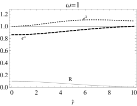
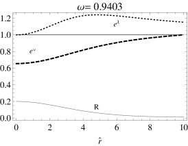
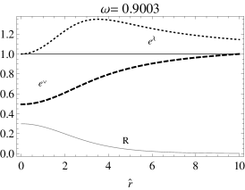
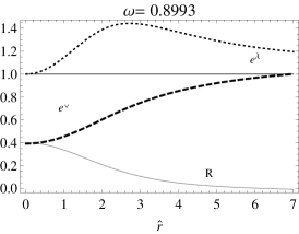
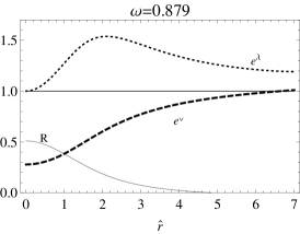
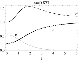
Figure 15: The radial function $R$ of the Klein–Gordon field (gray line), the metric coefficient $g_{11}=-e^{\lambda}$ (dotted line) and the function $e^{\nu}=g_{00}$ (dashed line) are plotted as functions of $\hat{r}$ (dimensionless) $\hat{r}=r/m$ for selected values of the redial function $R(r)$ at the origin and different values of the eigenvalue $\omega$ in units of $mc^{2}$.

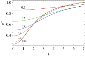
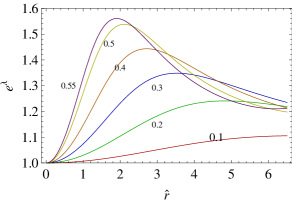
Figure 16: (Color online) The metric coefficient $g_{11}=-e^{\lambda}$ (right plot) and the function $e^{\nu}=g_{00}$ (left plot) are plotted as functions of $\hat{r}$ (dimensionless) $\hat{r}=r/m$ for selected values of the radial function $R(r)$ at the origin.

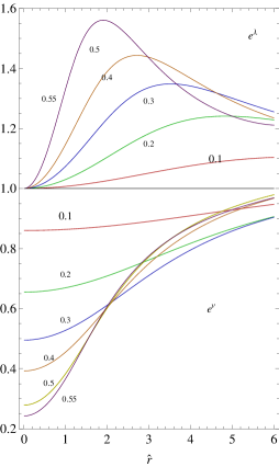
Figure 17: (Color online) The metric coefficient $e^{\lambda}=-g_{11}$ and the function $e^{\nu}=g_{00}$ are plotted as functions of $\hat{r}$ (dimensionless) $\hat{r}=r/m$ for selected values of the redial function $R(r)$ at the origin. See also Table 6.

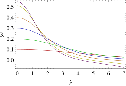
Figure 18: (Color online) The radial function $R$ is plotted as a function of $\hat{r}$ (dimensionless) $\hat{r}=r/m$ for selected values of $R$ at the origin. See also Table 6.

The mass at infinity and the total number of particle always stays positive. To an increase (decrease) of the number of particles always corresponds an increase (decrease) of the mass at infinity (see Fig. 19). The concept of critical mass is introduced since the total particle number and the mass at infinity (as a function of the central density, see Fig. 19) reaches a maximum value $N_{\mbox{\tiny{Cri}}}=0.658438M_{Pl}^{2}/m^{2}$ and $M_{\mbox{\tiny{Cri}}}=0.635626M_{Pl}^{2}/m$, respectively, for a specific central density $R(0)_{\mbox{\tiny{Cri}}}$:

$$N_{\mbox{\tiny{Cri}}}=0.658438M_{Pl}^{2}/m^{2},\qquad R(0)_{\mbox{\tiny{Cri}}}=0.278289,$$ (69)

$$M_{\mbox{\tiny{Cri}}}=0.635626M_{Pl}^{2}/m,\qquad R(0)_{\mbox{\tiny{Cri}}}=0.277619.$$ (70)

For further details, see also Jetzer:1988af .

Figure 19: The mass at infinity $M$ in units of $M_{Pl}^{2}/m$ (solid line), and the particle number $N$ in units of $M_{Pl}^{2}/m^{2}$ (dashed line) are plotted as functions of the central density $R(0)$. Note that there exists a maximum value of the mass $M\simeq 0.635626M_{Pl}^{2}/m$ for the central density $R(0)_{\mbox{\tiny{Cri}}}=0.277619$ above which there are no static solutions. There exists a maximum value of the particle number $N_{\mbox{\tiny{Cri}}}=0.658438M_{Pl}^{2}/m^{2}$ for the central density $R(0)_{\mbox{\tiny{Cri}}}=0.278289$.

References

- (1) F. E. Schunck and E. W. Mielke, Gen. Rel. Grav. 31, 787 (1999).
- (2) F. E. Schunck and E. W. Mielke, Phys. Lett. A 249, 389 (1998).
- (3) E. W. Mielke and F. E. Schunck, in Gravity, Particles and Space-Time ed P. Pronin and G. Sardanashvily, World Scientific: Singapore, pp 391-420 (1996).
- (4) S. U. Ji and S. J. Sin, Phys. Rev. D 50, 3655 (1994).
- (5) K. R. W. Jones and D. Bernstein, Class. Quantum Grav. 18, 1513 (2001).
- (6) C. Barceló, S. Liberati and M. Visser, Class. Quantum Grav. 18, 1137 (2001).
- (7) K. R W Jones and D. Bernstein, Class. Quantum Grav. 18, 8 1513 (2001).
- (8) P.-H. Chavanis, T. Harko, Phys. Rev. D 86, 064011 (2012).
- (9) P. Jetzer, P. Liljenberg and B. S. Skagerstam, Astropart. Phys. 1, 429 (1993).
- (10) B. Kleihaus, J. Kunz, C. Lammerzahl and M. List, Phys. Lett. B 675, 102 (2009).
- (11) D. F. Torres, S. Capozziello and G. Lambiase, Phys. Rev. D 62, 104012 (2000).
- (12) R. Ruffini, et. al. The Blackholic energy and the canonical Gamma-Ray Burst. In M. Novello S. E. Perez Bergliaffa, editor, XIIth Brazilian School of Cosmology and Gravitation, Vol. 910, American Institute of Physics Conference Series, pages 55–217, (2007).
- (13) S. L. Liebling and C. Palenzuela, Living Rev. Rel. 15, 6 (2012).
- (14) F. S. Guzman and J. M. Rueda-Becerril, Phys. Rev. D 80, 084023 (2009).
- (15) V. Gorini, A. Y. .Kamenshchik, U. Moschella and V. Pasquier, Phys. Rev. D 69, 123512 (2004).
- (16) C. Llinares and D. F. Mota, Phys. Rev. Lett. 110, 161101 (2013).
- (17) O. Bertolami and J. Paramos, Phys. Rev. D 71 023521 (2005).
- (18) S. Fay, Astron. Astrophys. 413, 799 - 805 (2004).
- (19) O. Bertolami, P. Carrilhom and J. P ramos, Phys. Rev. D 86, 103522 (2012).
- (20) C. Gao, M. Kunz, A. R. Liddle, and D. Parkinson, Phys. Rev. D 81, 043520 (2010).
- (21) R. Mainini, L. P. L. Colombo, and S. A. Bonometto, Astrophys. J. 632, 691 (2005).
- (22) A. Arbey EAS Publications Series 36, 161-166 (2009).
- (23) S. Chatrchyan et al. [CMS Collaboration], Phys. Lett. B 716, 30 (2012).
- (24) J. Polchinski, String theory (Cambridge University Press, Cambridge, UK, 1998).
- (25) R. Ruffini and S. Bonazzola, Phys. Rev. 187, 1767 (1969).
- (26) P. Jetzer and J. J. van der Bij, Phys. Lett. B 227, 341 (1989).
- (27) P. Jetzer, Phys. Lett. B 231, 433 (1989) .
- (28) P. Jetzer, CERN-TH-5681/90 (1990).
- (29) F. E. Schunck and E. W. Mielke, Class. Quant. Grav. 20, 301 (2003).
- (30) P. Jetzer, Nucl. Phys. B 16, 653 655 (1990).
- (31) P. Jetzer, Phys. Rept. 220, 163 (1992).
- (32) F. V. Kusmartsev, E. W. Mielke and F. E. Schunck, Phys. Rev. D 43, 3895 (1991).
- (33) F. E. Schunck and E. W. Mielke, Gen. Rel. Grav. 31, 787 (1999).
- (34) E. W. Mielke and F. E. Schunck, arXiv:gr-qc/9801063.
- (35) S. A. Fulling, Aspects of quantum field theory in curved space-time, CUP Cambridge University Press (1989).
- (36) N. D. Birrell and P. C. W. Davies, Quantum fields in curved space, CUP Cambridge University Press (1982).
- (37) A. B. Adib, arXiv:hep-th/0208168.
- (38) G. H. Derrick, J. Math. Phys. 5, 1252 (1964).
- (39) P. Jetzer and D. Scialom, arXiv:gr-qc/9709056 (1997).
- (40) M. Wyman, Phys. Rev. D 24, 839 (1981).
- (41) A. Prikas, Phys. Rev. D 66, 025023 (2002).
- (42) P. Jetzer, Phys. Lett. B 222, 447 (1989).
- (43) P. Jetzer, Nucl. Phys. Proc. Suppl. 14B, 265 (1990).
- (44) P. Jetzer, in 5th Marcel Grossmann Meeting on General Relativity, pt.B, Perth, Australia, 1988, pp.1249-1254.
- (45) P. Jetzer, Nucl. Phys. B 316, 411 (1989).
- (46) P. Jetzer, Phys. Lett. B 243,36 (1990).
- (47) B. Kleihaus, J. Kunz and S. Schneider, Phys. Rev. D 85, 024045 (2012).
- (48) S. Hod, Phys. Lett. B 693, 339 (2010).
- (49) J. Madsen, Phys. Rev. Lett. 100,151102 (2008).
- (50) K. Eilers, B. Hartmann, V. Kagramanova, I. Schaffer and C. Toma, arXiv:1304.5646.
- (51) B. Hartmann and J. Riedel, Phys. Rev. D 87, 044003 (2013).