Relay Selection for Bidirectional AF Relay Network with Outdated CSI

Abstract

Most previous researches on bidirectional relay selection (RS) typically assume perfect channel state information (CSI). However, outdated CSI, caused by the the time-variation of channel, cannot be ignored in the practical system, and it will deteriorate the performance. In this paper, the effect of outdated CSI on the performance of bidirectional amplify-and-forward RS is investigated. The optimal single RS scheme in minimizing the symbol error rate (SER) is revised by incorporating the outdated channels. The analytical expressions of end-to-end signal to noise ratio (SNR) and symbol error rate (SER) are derived in a closed-form, along with the asymptotic SER expression in high SNR. All the analytical expressions are verified by the Monte-Carlo simulations. The analytical and the simulation results reveal that once CSI is outdated, the diversity order degrades to one from full diversity. Furthermore, a multiple RS scheme is proposed and verified that this scheme is a feasible solution to compensate the diversity loss caused by outdated CSI.

I Introduction

Recently, bidirectional relay communications, in which two sources exchange information through the intermediate relays, have attracted a lot of attention, and different transmission schemes of bidirectional relay have been proposed in[1, 2, 3]. An amplify-and-forward (AF) based network coding scheme, named as analog network coding (ANC), was introduced in [3]. With ANC, the data transmission of bidirectional AF relay can be divided into two phases, and the spectral efficiency can get improved [3]. Recently, relay selection (RS) technique for bidirectional relay networks has been intensively researched, due to its ability to achieve full diversity with only one relay[5, 7, 4, 6, 9]. Performing RS, the best relay is firstly selected before data transmission, according to the predefined RS scheme. In [4], a optimal RS scheme in minimizing the average symbol error rate (SER) for the source pair was proposed, and the bounds of SER and the optimal power allocation scheme were provided. The author in [5] derived the tight lower bound of block error rate for the bidirectional RS network. The performance bounds, such as the average sum rate and outage probability, for the bidirectional RS was offered under the Rayleigh fading in [6], and these bounds were extended to the Nakagami-m fading in [7]. In [8], a relay-assisted bidirectional cellular network was considered, and a resource allocation method, including the optimal relay selection scheme, was proposed to improve the overall system performance. The diversity order for various RS schemes of bidirectional RS was studied in [9], and it proved that the RS schemes can achieve full diversity when the channel state information (CSI) is perfect.

Furthermore, all the aforementioned researches analyzed the bidirectional RS with perfect CSI. Outdated CSI, caused by the time-variation of channel, cannot be negligible in the practical system, and it makes the selected relay not the best for the data transmission. The impact of outdated CSI has been fully discussed in one-way RS[10, 11, 12, 13]. In [10, 11], the expressions of SER and outage probability for one-way AF RS were obtained, and the partial RS and opportunistic RS were both considered with outdated CSI. The impact of outdated CSI and channel estimation error on the one-way decode-and-forward (DF) RS was analyzed in [12]. Multiple RS with AF and DF protocols was considered in one-way relay with outdated CSI [13], in which the outage probability and diversity order were analyzed. In [14], the two-way network with one relay and multiple users was studied, and the effect of outdated CSI on user selection was researched. In [15], the antenna selection criterion of MIMO two-way relay was proposed, and the performance with outdated CSI was analyzed when there are one single-antenna relay.

However, to the best of the authors’ knowledge, the impact of outdated CSI on the performance of bidirectional RS has not been investigated. In this paper, we analyze the SER performance of the bidirectional AF RS with outdated CSI. The optimal single RS in minimizing the instantaneous SER is revised by incorporating the outdated channels. The distribution of end-to-end signal-to-noise ratio (SNR), the analytical average SER expressions are derived in this paper, and verified by the Monte-Carlo simulations. The effect of the parameters, such as the number of relays and the correlation coefficient of outdated CSI, are investigated. The theoretical analysis and the simulation results reveal that once CSI is outdated, the diversity order reduces to one, regardless of the number of relays. Furthermore, a multiple RS scheme for the bidirectional relay is proposed to improve the diversity loss.

In summary, the main contribution of this paper is listed as follows:

1. Outdated CSI is taken into account to derive the analytical results of bidirectional RS, and its therein impact is investigated.

2. Considering the generalized network structure, i.e., different channels have different variances and different correlation coefficients of outdated CSI, the generalized average SER expression is obtained, which can be further simplified according to the concrete situations, such as high SNR analysis and the analysis of symmetric network.

3. The SER expression derived in this paper is tight with the exact result, and verified by the Monte-Carlo simulations.

4. A multiple RS scheme by selecting the best $K$ relays from $N$ available relays is proposed in the bidirectional relay, and the diversity order is analyzed, which reveals that the multiple RS can compensate the diversity loss caused by outdated CSI.

The remainder of this paper is organized as follows: In Section II, the system model of bidirectional AF RS, the outdated CSI model, and the RS schemes are described in detail. Section III provides the analytical expressions of bidirectional RS, including the distribution function of received SNR, the performance of end-to-end average SER, and the diversity order. Simulation results and performance analysis are presented in Section IV. Finally, Section V concludes this paper.

Notation: $\left|\cdot\right|$ represents the absolute value, $\mathbb{E}$ is used for the expectation, and $\Pr$ represents the probability. The probability density function (PDF) and the cumulative probability function (CDF) of random variable (RV) $x$ are denoted by $f_{x}\left(\cdot\right)$ and $F_{x}\left(\cdot\right)$, respectively.

II System Model

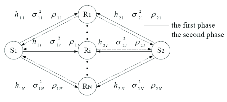
Figure 1: System model of bidirectional relay network.

As shown in Fig. 1, the system investigated in this paper is a bidirectional AF relay network with two sources $S_{j}$, $j=1,2$, exchanging information through $N$ relays $R_{i}$, $i=1,\ldots,N$, in which each communication node is equipped with a single half-duplex antenna. The transmit powers of each source and each relay are denoted by $p_{s}$ and $p_{r}$, respectively. The direct link between the sources does not exist due to the shadowing effect, and the channel coefficients between $S_{j}$ and $R_{i}$ are reciprocal, denoted by $h_{ji}$. All the channel coefficients follow independent complex-Gaussian distribution with zero mean and variance of $\sigma_{ji}^{2}$.

II-A Instantaneous Received SNR at the Sources

Considering the transmission via $R_{i}$, the data transmission of bidirectional AF relay is divided into two phases. During the first phase, the sources simultaneously send their respective information to $R_{i}$. The received signal at $R_{i}$ is $r_{i}=\sqrt{p_{s}}h_{1i}s_{1}+\sqrt{p_{s}}h_{2i}s_{2}+n_{ri}$, where $s_{j}$ denotes the modulated symbols transmitted by $S_{j}$ with the average power normalized, and $n_{ri}$ is the additive white Gaussian noise (AWGN) at $R_{i}$, with zero mean and variance of $\sigma_{n}^{2}$. During the second phase, $R_{i}$ amplifies the received signal and forwards it back to the sources. The signal generated by $R_{i}$ satisfies $t_{i}=\sqrt{p_{r}}\beta_{i}r_{i}$, where $\beta_{i}=\left(p_{s}|h_{1i}|^{2}+p_{s}|h_{2i}|^{2}+\sigma_{n}^{2}\right)^{-1/2}$ is the variable-gain factor[4]. The received signal at $S_{j}$, $j=1,2$, is $y_{j}=h_{ji}t_{i}+n_{sj}$, where $n_{sj}$ is the AWGN at $S_{j}$. Then, after canceling the self-interference, i.e., $\sqrt{p_{s}p_{r}}\beta_{i}h_{ji}h_{ji}s_{j}$, the instantaneous received SNR at $S_{j}$ via $R_{i}$ is[4]

$$\gamma_{ji}=\frac{{\psi_{s}\psi_{r}\left|{h_{ji}}\right|^{2}\left|{h_{\bar{j}i}}\right|^{2}}}{{\left({\psi_{s}+\psi_{r}}\right)\left|{h_{ji}}\right|^{2}+\psi_{s}\left|{h_{\bar{j}i}}\right|^{2}+1}}$$ (1)

where $\psi_{s}=p_{s}/\sigma_{n}^{2}$, $\psi_{r}=p_{r}/\sigma_{n}^{2}$, and $\{j,\overline{j}\}=\{1,2\}~{}\mbox{or}~{}\{2,1\}$.

Furthermore, by ignoring the constant $1$ in the denominator of (1), we can obtain the upper bound of received SNR, i.e.,

$$\gamma_{ji}=\frac{{\left({\psi_{r}\left|{h_{ji}}\right|^{2}}\right)\left({\psi_{h}\left|{h_{\bar{j}i}}\right|^{2}}\right)}}{{\left({\psi_{r}\left|{h_{ji}}\right|^{2}}\right)+\left({\psi_{h}\left|{h_{\bar{j}i}}\right|^{2}}\right)}}$$ (2)

where $\psi_{h}=\psi_{s}\psi_{r}/\left(\psi_{s}+\psi_{r}\right)$. This bound is tight enough with the exact result, especially in high SNR. Therefore, in the following, we use the bound for analysis [4].

II-B Relay Selection Schemes

To minimize the instantaneous SER for the source pair, the index of the selected relay should satisfy[4]

$$k=\arg\max_{i}\min\left\{\gamma_{1i},\gamma_{2i}\right\}$$ (3)

where $\gamma_{ji}$ is decided by (2).

Before further discussion and analysis, we provide the following Lemma.

Lemma 1: The minimization of $\gamma_{1i}$ and $\gamma_{2i}$ is bounded by

$$\min\left(\gamma_{1i},\gamma_{2i}\right)\leq\frac{\psi_{s}\psi_{r}}{\psi_{s}+\psi_{r}}\min\left(|h_{1i}|^{2},|h_{2i}|^{2}\right)$$ (4)

where the right-hand side of (4) is the upper bound of the left-hand side, and it is also a tight approximation, especially in high SNR.

Proof: The derivation is given in Appendix A.$\hfill\blacksquare$

According to Lemma 1 and (3), the optimal RS scheme in minimizing the instantaneous SER for the source pair is equivalent to [5, 7]

$$k=\arg\max_{i}\min\left\{|h_{1i}|^{2},|h_{2i}|^{2}\right\}.$$ (5)

Specifically, the relay selection can be achieved in the distributed or centralized manner.

If the relay selection is conducted in the distributed manner [16, 17], each relay $R_{i}$ estimates the local channel coefficients $h_{1i}$ and $h_{2i}$, by the exchanges of control packets, such as, ready-to-send and clear-to-send frames [16]. The concrete estimation method can be found in [18], which is beyond the scope of this paper. In the selection process, the timer mechanism is employed among the available relays to determine the “best” relay autonomously [16]. In this procedure, the delay between relay selection and data transmission takes up about one cooperation phase [17], which may subject to relatively serious channel variations, and thus the CSI is outdated.

If the relay selection is conducted in the centralized manner [10], the central unit, such as, the source $S_{1}$, estimates all the links’ channel coefficients, with the help of the pilots from the other source $S_{2}$. The concrete estimation method can be found in [10]. Based on the estimated channel coefficients, the “best” relay is selected, according to the predefined RS schemes. Then, the central unit broadcasts the index of the selected relay to all the relays. In this procedure, the delay between relay selection and data transmission also exists, due to the feedback delay [10], and thus the CSI is also outdated.

In summary, because of the feedback delay and the scheduling delay, the selection of the best relay is not based on the current time instant[10], regardless of centralized and distributed relay selection. The channel coefficient at the selection instant is denoted by $\hat{h}_{ji}$. Due to the time-variation of channel, $\hat{h}_{ji}$ is outdated to $h_{ji}$, and their relationship is decided by the Jakes’ model[10]

$$\hat{h}_{ji}=\rho_{ji}h_{ji}+\sqrt{1-{\rho_{ji}^{2}}}\varepsilon_{ji}$$ (6)

where $\varepsilon_{ji}$ is an independent identically distributed RV with $h_{ji}$, the correlation coefficient $\rho_{ji}=J_{0}\left(2\pi f_{d_{ji}}T_{d}\right)$, where $J_{0}\left(\cdot\right)$ stands for the zeroth order Bessel function[22], $f_{d_{ji}}$ is the Doppler spread, and $T_{d}$ is the time delay between $\hat{h}_{ji}$ and $h_{ji}$. Moreover, $\rho_{{ji}}=1$, i.e., $f_{d_{ji}}=0$, means CSI is perfect, and $\rho_{{ji}}<1$, i.e., $f_{d_{ji}}>0$, means CSI is outdated.

Therefore, the RS scheme (5) with outdated CSI is converted into

$$k=\arg\max_{i}\min\left\{|\hat{h}_{1i}|^{2},|\hat{h}_{2i}|^{2}\right\}.$$ (7)

In the following, we analyze the performance of the RS scheme (7) with outdated CSI, and the performance with perfect CSI can be obtained by setting $\rho_{ji}=1$.

III Performance Analysis of Bidirectional Relay Selection with Outdated CSI

In the following, the analytical and asymptotic average SER expressions of the single RS scheme (7) are derived in a closed-form.

III-A The Distribution of end-to-end Received SNR

To analyze the performance of bidirectional AF single RS (7), the distribution function of $\gamma_{jk}$ in (2) is required. Therefore, the analytical PDF and CDF of (2) with outdated CSI are derived in this part.

In order to obtain the exact distribution of (2), we need to achieve the distribution of $\left|{h_{j{k}}}\right|^{2}$, which is decided by $\left|\hat{h}_{jk}\right|^{2}$, according to (6). Moreover, $\left|\hat{h}_{jk}\right|^{2}$ is decided by the RS scheme (7). After some manipulation, we can obtain

Lemma 2: The PDF of $\left|{h_{jk}}\right|^{2}$, $\left\{j,\overline{j}\right\}=\left\{1,2\right\}~{}\mbox{or}~{}\left\{1,2\right\}$ is

$$f_{\left|{h_{jk}}\right|^{2}}\left(z\right)=\sum\limits_{i=1}^{N}{\sum\limits_{t=0}^{N-1}{\sum\limits_{A_{t}}{\left({-1}\right)^{t}\left({1+\sum\limits_{l\in A_{t}}{\frac{{\sigma_{\bar{j}i}^{2}}}{{\sigma_{l}^{2}}}}}\right)}}^{-1}}\bigg{[}\frac{1}{{\sigma_{ji}^{2}}}\exp\left({-\frac{z}{{\sigma_{ji}^{2}}}}\right)+\frac{{\zeta_{j}}}{{\sigma_{ji}^{2}}}\exp\left({-\frac{{\xi_{j}}}{{\sigma_{ji}^{2}}}z}\right)\bigg{]}$$ (8)

where

$$\xi_{j}=\left({\frac{1}{{\sigma_{i}^{2}}}+\sum\limits_{l\in A_{t}}{\frac{1}{{\sigma_{l}^{2}}}}}\right)\left({\frac{{\rho_{ji}^{2}}}{{\sigma_{ji}^{2}}}+\frac{{1-\rho_{ji}^{2}}}{{\sigma_{i}^{2}}}+\sum\limits_{l\in A_{t}}{\frac{{1-\rho_{ji}^{2}}}{{\sigma_{l}^{2}}}}}\right)^{-1},$$ (9)

$$\zeta_{j}=\left({\frac{{\sigma_{\bar{j}i}^{2}}}{{\sigma_{ji}^{2}}}\sum\limits_{l\in A_{t}}{\frac{1}{{\sigma_{l}^{2}}}}}\right)\left({\frac{{\rho_{ji}^{2}}}{{\sigma_{ji}^{2}}}+\frac{{1-\rho_{ji}^{2}}}{{\sigma_{i}^{2}}}+\sum\limits_{l\in A_{t}}{\frac{{1-\rho_{ji}^{2}}}{{\sigma_{l}^{2}}}}}\right)^{-1}.$$ (10)

In addition, $\sum\limits_{A_{t}}$ is the abbreviation of $\sum\limits_{\scriptstyle A_{t}\subseteq\left\{{1,\ldots,N}\right\}\backslash i\hfill\atop\scriptstyle\left|{A_{t}}\right|=t\hfill}$, $\left|{A_{t}}\right|$ represents the cardinality of set $A_{t}$, and $\sigma_{i}^{2}=\sigma_{1i}^{2}\sigma_{2i}^{2}/\big{(}\sigma_{1i}^{2}+\sigma_{2i}^{2}\big{)}$ $i=1,\ldots,N$.

Proof: The derivation is given in Appendix B. $\hfill\blacksquare$

Before deriving the distribution of received SNR, we introduce two equations, which are necessary for the following analysis.

Lemma 3:

$$\sum\limits_{i=1}^{N}{\sum\limits_{t=0}^{N-1}{\sum\limits_{A_{t}}{\left({-1}\right)^{t}\left({\sum\limits_{l\in A_{t}}{\frac{{\sigma_{i}^{2}}}{{\sigma_{l}^{2}}}+1}}\right)^{-1}}}}=1,\mbox{and}\sum\limits_{t=1}^{N-1}{\sum\limits_{A_{t}}{\left({-1}\right)^{t}\left({\sum\limits_{l\in A_{t}}{\frac{1}{{\sigma_{l}^{2}}}}}\right)^{k}}}=0,0\leq k\leq N-2.$$ (11)

Proof: The derivation is given in Appendix C. $\hfill\blacksquare$

According to Lemma 3, we can obtain the CDF of $|h_{jk}|^{2}$, $j=1,2$, by integrating the PDF in Lemma 2. Also, the PDF and CDF of $\Omega_{1}=\psi_{r}|h_{jk}|^{2}$ and $\Omega_{2}=\psi_{h}|h_{\overline{j}k}|^{2}$ in (2) can be obtained by the fact that when $Y=mX\left(m>0\right)$, $f_{Y}\left(z\right)=\left({1}/{m}\right)f_{X}\left({z}/{m}\right)$ and $F_{Y}\left(z\right)=F_{X}\left({z}/{m}\right)$[24].

Proposition 1: With the definition that

$$a_{i}=\frac{1}{{\psi_{r}\sigma_{ji}^{2}}}~{},~{}b_{i^{\prime}}=\frac{1}{{\psi_{h}\sigma_{\bar{j}i^{\prime}}^{2}}},$$ (12)

the CDF of the received SNR at $S_{j}$ via the selected relay $R_{k}$ is

$$F_{\gamma_{jk}}\left(z\right)=1-\sum\limits_{i=1}^{N}{\sum\limits_{t=0}^{N-1}{\sum\limits_{A_{t}}{\sum\limits_{i^{\prime}=1}^{N}{\sum\limits_{t^{\prime}=0}^{N-1}{\sum\limits_{A_{t^{\prime}}}{\left({-1}\right)^{t+t^{\prime}}\left({1+\sum\limits_{l\in A_{t}}{\frac{{\sigma_{\bar{j}i}^{2}}}{{\sigma_{l}^{2}}}}}\right)^{-1}\left({1+\sum\limits_{l^{\prime}\in A_{t^{\prime}}}{\frac{{\sigma_{ji^{\prime}}^{2}}}{{\sigma_{l^{\prime}}^{2}}}}}\right)^{-1}\sqrt{4a_{i}b_{i^{\prime}}}}}}}}}$$

$$\hskip 182.09763pt\times\left({f_{11}+f_{12}+f_{21}+f_{22}}\right)$$ (13)

where

$$f_{11}=z\exp\left({-a_{i}z-b_{i^{\prime}}z}\right)K_{1}\left({2z\sqrt{a_{i}b_{i^{\prime}}}}\right),$$ (14)

$$f_{12}=\frac{\zeta^{\prime}_{\bar{j}}}{\sqrt{\xi^{\prime}_{\bar{j}}}}z\exp\left(-a_{i}z-\xi^{\prime}_{\bar{j}}b_{i^{\prime}}z\right)K_{1}\left(2z\sqrt{\xi^{\prime}_{\bar{j}}a_{i}b_{i^{\prime}}}\right),$$ (15)

$$f_{21}=\frac{{\zeta_{j}}}{{\sqrt{\xi_{j}}}}z\exp\left({-a_{i}\xi_{j}z-b_{i^{\prime}}z}\right)K_{1}\left({2z\sqrt{\xi_{j}a_{1i}b_{i^{\prime}}}}\right),$$ (16)

and

$$f_{22}=\frac{{\zeta^{\prime}_{\bar{j}}\zeta_{j}}}{{\sqrt{\xi^{\prime}_{\bar{j}}\xi_{j}}}}z\exp\left({-\xi_{j}a_{i}z-\xi^{\prime}_{\bar{j}}b_{i^{\prime}}z}\right)K_{1}\left({2z\sqrt{\xi_{j}\xi^{\prime}_{\bar{j}}a_{i}b_{i^{\prime}}}}\right).$$ (17)

In addition, $\{j,\overline{j}\}=\{1,2\}~{}\mbox{or}~{}\{2,1\}$, $\sum\limits_{A_{t^{\prime}}}$ is the abbreviation of $\sum\limits_{\scriptstyle A_{t^{\prime}}\subseteq\left\{{1,\ldots,N}\right\}\backslash i^{\prime}\hfill\atop\scriptstyle\left|{A_{t^{\prime}}}\right|=t^{\prime}\hfill}$, $\xi^{\prime}_{j}$ and $\zeta^{\prime}_{j}$ can be obtained by $\xi_{j}$ and $\zeta_{j}$, respectively, by substituting $i,l,A_{t}$ in (9) and (10) with $i^{\prime},l^{\prime},A_{t^{\prime}}$, respectively, and $K_{1}\left(\cdot\right)$ is the first order modified Bessel function of the second kind[22].

Proof: The derivation is given in Appendix D.$\hfill\blacksquare$

III-B Analytical Average SER Analysis of the RS Scheme (7) with Outdated CSI

For many common linear modulation formats, the average SER can be obtained by [11]

$$\overline{SER}=\alpha\mathbb{E}\left[Q\left(\sqrt{\beta\gamma}\right)\right]=\frac{\alpha}{{\sqrt{2\pi}}}\int\limits_{0}^{\infty}{F_{\gamma}\left(\frac{{t^{2}}}{\beta}\right)e^{-\frac{{t^{2}}}{2}}}dt$$ (18)

where $\gamma$ is the instantaneous received SNR, $Q\left(\cdot\right)$ is the Gaussian Q-Function[22], and $\left(\alpha,\beta\right)$ are decided by the modulation formats[11], e.g., $\left(\alpha,\beta\right)=\left(1,2\right)$ for BPSK.

Proposition 2: Substituting Proposition $1$ into (18), the average SER expression of $S_{j}$ is obtained

$$\overline{SER}_{j}=\frac{\alpha}{2}-\frac{{3\sqrt{2}\pi\alpha\sqrt{\beta}}}{2}\sum\limits_{i=1}^{N}{\sum\limits_{t=0}^{N-1}{\sum\limits_{A_{t}}{\sum\limits_{i^{\prime}=1}^{N}{\sum\limits_{t^{\prime}=0}^{N-1}{\sum\limits_{A_{t^{\prime}}}{\left({-1}\right)^{t+t^{\prime}}\left({1+\sum\limits_{l\in A_{t}}{\frac{{\sigma_{\bar{j}i}^{2}}}{{\sigma_{l}^{2}}}}}\right)^{-1}\left({1+\sum\limits_{l^{\prime}\in A_{t^{\prime}}}{\frac{{\sigma_{ji^{\prime}}^{2}}}{{\sigma_{l^{\prime}}^{2}}}}}\right)^{-1}a_{i}b_{i^{\prime}}}}}}}}$$

$$\hskip 239.00314pt\times\left({g_{11}+g_{12}+g_{21}+g_{22}}\right)$$ (19)

where

$$g_{11}=\left[{\left({\sqrt{a_{i}}+\sqrt{b_{i^{\prime}}}}\right)^{2}+\frac{\beta}{2}}\right]^{-\frac{5}{2}}F\left({\frac{5}{2},\frac{3}{2};2;\frac{{\left({\sqrt{a_{i}}-\sqrt{b_{i^{\prime}}}}\right)^{2}+\frac{\beta}{2}}}{{\left({\sqrt{a_{i}}+\sqrt{b_{i^{\prime}}}}\right)^{2}+\frac{\beta}{2}}}}\right),$$ (20)

$$g_{12}=\zeta^{\prime}_{\bar{j}}\left[{\left({\sqrt{a_{i}}+\sqrt{\xi^{\prime}_{\bar{j}}b_{i^{\prime}}}}\right)^{2}+\frac{\beta}{2}}\right]^{-\frac{5}{2}}F\left({\frac{5}{2},\frac{3}{2};2;\frac{{\left({\sqrt{a_{i}}-\sqrt{\xi^{\prime}_{\bar{j}}b_{i^{\prime}}}}\right)^{2}+\frac{\beta}{2}}}{{\left({\sqrt{a_{i}}+\sqrt{\xi^{\prime}_{\bar{j}}b_{i^{\prime}}}}\right)^{2}+\frac{\beta}{2}}}}\right),$$ (21)

$$g_{21}=\zeta_{j}\left[{\left({\sqrt{\xi_{j}a_{i}}+\sqrt{b_{i^{\prime}}}}\right)^{2}+\frac{\beta}{2}}\right]^{-\frac{5}{2}}F\left({\frac{5}{2},\frac{3}{2};2;\frac{{\left({\sqrt{\xi_{j}a_{i}}-\sqrt{b_{i^{\prime}}}}\right)^{2}+\frac{\beta}{2}}}{{\left({\sqrt{\xi_{j}a_{i}}+\sqrt{b_{i^{\prime}}}}\right)^{2}+\frac{\beta}{2}}}}\right),$$ (22)

and

$$g_{22}=\zeta_{j}\zeta^{\prime}_{\bar{j}}\left[{\left({\sqrt{\xi_{j}a_{i}}+\sqrt{\xi^{\prime}_{\bar{j}}b_{i^{\prime}}}}\right)^{2}+\frac{\beta}{2}}\right]^{-\frac{5}{2}}F\left({\frac{5}{2},\frac{3}{2};2;\frac{{\left({\sqrt{\xi_{j}a_{i}}-\sqrt{\xi^{\prime}_{\bar{j}}b_{i^{\prime}}}}\right)^{2}+\frac{\beta}{2}}}{{\left({\sqrt{\xi_{j}a_{i}}+\sqrt{\xi^{\prime}_{\bar{j}}b_{i^{\prime}}}}\right)^{2}+\frac{\beta}{2}}}}\right).$$ (23)

In addition, $F\left(a,b,;c;z\right)$ is the Confluent Hypergeometric function[22].

Proof: The derivation is given in Appendix D.$\hfill\blacksquare$

Proposition 2 provides the generalized average SER expression. However, this expression of average SER in Proposition 2 is too complicated, thus we resort to the asymptotic analysis to simplify the expression.

III-C Asymptotic Average SER Analysis in high SNR

Corollary 1: By Lemma 3 and Proposition 2, the asymptotic average SER of $S_{j}$, $\left\{j,\overline{j}\right\}=\left\{1,2\right\}~{}\mbox{or}~{}\left\{2,1\right\}$, in high SNR is

$\left(1\right)$ If CSI is perfect, i.e., $f_{d_{ji}}=0$

$$\overline{SER}_{j}^{\infty}=\frac{\alpha}{{2\sqrt{\pi}}}\left({\frac{2}{\beta}}\right)^{N}\frac{{\Gamma\left({1/2+N}\right)}}{{\Gamma\left({N+1}\right)}}\sum\limits_{i=1}^{N}{\sum\limits_{t=0}^{N-1}{\sum\limits_{A_{t}}{\left({-1}\right)^{N+t+1}}}}$$

$$\hskip 85.35826pt\times\left[{\left({\sum\limits_{l\in A_{t}}{\frac{{\sigma_{ji}^{2}}}{{\sigma_{l}^{2}}}}}\right)^{N-1}\left({\frac{1}{{\psi_{r}\sigma_{ji}^{2}}}}\right)^{N}+\left({\sum\limits_{l\in A_{t}}{\frac{{\sigma_{\bar{j}i}^{2}}}{{\sigma_{l}^{2}}}}}\right)^{N-1}\left({\frac{1}{{\psi_{h}\sigma_{\bar{j}i}^{2}}}}\right)^{N}}\right]$$ (24)

where $\Gamma\left(\cdot\right)$ is the Gamma function[22].

$\left(2\right)$ If CSI is outdated, i.e., $f_{d_{ji}}>0$

$$\overline{SER_{j}}^{\infty}=\frac{\alpha}{{2\beta}}\sum\limits_{i=1}^{N}{\sum\limits_{t=0}^{N-1}{\sum\limits_{A_{t}}{\left({-1}\right)^{t}}}}\left[\frac{{1+\zeta_{j}}}{{1+\sum\limits_{l\in A_{t}}{\frac{{\sigma_{\bar{j}i}^{2}}}{{\sigma_{l}^{2}}}}}}\frac{1}{{\psi_{r}\sigma_{ji}^{2}}}{\rm{}}+\frac{{1+\zeta_{\bar{j}}}}{{1+\sum\limits_{l\in A_{t}}{\frac{{\sigma_{ji}^{2}}}{{\sigma_{l}^{2}}}}}}\frac{1}{{\psi_{h}\sigma_{\bar{j}i}^{2}}}\right].$$ (25)

Proof: The derivation is given in Appendix E.$\hfill\blacksquare$

Furthermore, it is worthy of noting that the previous analytical expressions, i.e., from Lemma 1 to Corollary 1, are all obtained under the generalized network structure, i.e., the variances $\sigma_{ji}^{2}$ and the correlation coefficients $\rho_{ji}$ for different channels are different. If the network structure is symmetric, i.e., $\sigma_{ji}^{2}=1$ and $\rho_{ji}=\rho$, the previous expressions can be further simplified by $\sum\limits_{i=1}^{N}\to N$, $\sum\limits_{A_{t}}\to\binom{N-1}{t}$, and $\sum\limits_{l\in A_{t}}\to t$.

III-D Diversity Analysis of Single and Multiple RS Schemes with Outdated CSI

With the aid of the asymptotic SER expressions, diversity order $d$, which implies the slope of SER in log-log scale when SNR approaches infinity[21], satisfies

Corollary 2:

$$d=\begin{cases}N,~{}\text{CSI is perfect};\\ 1,~{}\text{CSI is outdated}.\end{cases}$$ (26)

Proof: The proof is given in Appendix E.$\hfill\blacksquare$

Corollary 2 reveals that the diversity order of the single relay selection scheme (7) degrades to one from full diversity, once the CSI is outdated.

To compensate the diversity loss, a multiple RS scheme with outdated CSI by selecting the best $K$ relays from the $N$ available relays is proposed.

Assuming $\varphi^{(K)}$ to be the $K$th largest value among the set $\big{\{}\varphi_{i}\buildrel\Delta\over{=}\min\big{(}|\hat{h}_{1i}|^{2},|\hat{h}_{2i}|^{2}\big{)},i=1,\ldots,N\big{\}}$, the relay $R_{i}$, $i=1,\ldots,N$, is selected if and only if

$$\varphi_{i}\geq\varphi^{(K)}.$$ (27)

The selected $K$ relays can forward the signals in the orthogonal resources, and the maximal ratio combing is adopted at the sources.

Proposition 3: Selecting the best $K$ relays from $N$ available relays by the RS scheme (27) and using the maximal-ratio combining, the diversity order is

$$d=\begin{cases}N,~{}\text{CSI is perfect};\\ K,~{}\text{CSI is outdated}.\end{cases}$$ (28)

Proof: The proof is given in Appendix F.$\hfill\blacksquare$

Therefore, increasing the number of selected relay $K$ results in the improvement of diversity order in high SNR, thus the average SER performance also gets improved.

It is worthy point out that from the perspective of diversity order, multiple RS is not better than single RS when CSI is perfect, because they both can achieve the full diversity, and single RS only exploits one relay [20]. Nevertheless, multiple RS can improve the diversity order with outdated CSI, in comparison with single RS [13].

IV Simulation Results and Discussion

In this section, Monte-Carlo simulations are provided to validate the preceding analysis and to highlight the performance of bidirectional AF RS with outdated CSI. Without loss of generality, the average SER of the simulation results only concern about $S_{1}$ under BPSK modulation. Moreover, the variance of the channel satisfies $\sigma_{{ji}}^{2}=1$, and the Doppler spread of the channel satisfies $f_{d_{ji}}=f_{d}$, $i=1,\ldots,N$, and $j=1,2$.

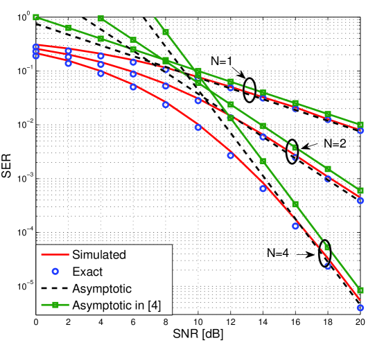
Figure 2: SER of $S_{1}$ when CSI is perfect and $N=1,2,4$.

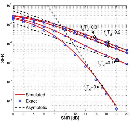
Figure 3: SER of $S_{1}$ when CSI is outdated and $N=4$.

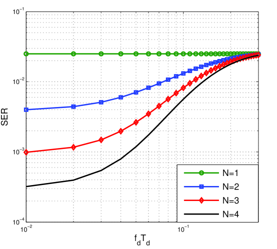
Figure 4: The impact of $f_{d}T_{d}$ on the SER when $\mbox{SNR}=15$ dB and $N=1,2,3,4$.

Figs. 2-5 investigate the performance of single RS scheme (7), in which each source and each relay are assumed to have the same transmit powers, i.e., $p_{s}=p_{r}=P_{0}$.

In Fig. 2, the simulation and the analytical SER of bidirectional RS are provided with perfect CSI, i.e, $f_{d}T_{d}=0$, when the number of relays $N=1,2,4$. The x-axis of this figure is $\mbox{SNR}=P_{0}/\sigma_{n}^{2}$ in dB. This figure reveals that increasing the number of relays can reduce the average SER, because the diversity order is $N$ when CSI is perfect, which satisfies the result of Corollary 2. From this figure, the exact SER expression of Proposition 2 is verified when CSI is perfect, in which the exact analytical expression of SER tightly matches with the simulation results than the previous researches[4], and the asymptotic results obtained from Corollary 1 also converges to the simulation results in high SNR.

Fig. 3 studies the impact of outdated CSI on the SER performance when $N=4$ and $f_{d}T_{d}=0,0.1,0.2,0.3$. The x-axis of this figure is $\mbox{SNR}=P_{0}/\sigma_{n}^{2}$ in dB. Different lines are provided under different $f_{d}T_{d}$, where larger $f_{d}T_{d}$ means CSI is severely outdated, whereas smaller $f_{d}T_{d}$ means CSI is slightly outdated, and especially $f_{d}T_{d}=0$ means CSI is perfect. The figure verifies the expressions of Proposition 2 and Corollary 1 when CSI is outdated. The figure also presents the adverse effect of outdated CSI on the performance: if and only if CSI is perfect, the diversity order is $N$; however, once CSI is outdated, the performance degrades greatly that the diversity order reduces to $1$, which satisfies Corollary $2$. The qualitative explanation of the phenomenon is that once CSI is outdated, it is quite possible that the worst relay can be selected, and hence diversity order is $1$. Furthermore, although diversity order is the same for any $f_{d}T_{d}>0$, the performance loss is smaller for smaller $f_{d}T_{d}$. Specifically, the gap of SER between $f_{d}T_{d}=0.1$ and $f_{d}T_{d}=0.2$ is about $4$ dB in high SNR.

Fig. 4 investigates the impact of $f_{d}T_{d}$ on SER when $\mbox{SNR}=15$ dB and the number of relays $N=1,2,3,4$. As the figure reveals, the SER gets worse as the CSI becomes severely outdated. During the range of small $f_{d}T_{d}$, the SER of larger $N$ still have significant gain over the SER of smaller $N$, whereas all the curves approach to the performance of $N=1$ as $f_{d}T_{d}$ increases. This indicates that with severely outdated CSI, no significant performance gain can be achieved by deploying more relays. Therefore, the RS scheme (7) behaves as the random RS, when the CSI is severely outdated.

Fig. 5 plots the diversity order of finite SNR [12] when $f_{d}T_{d}=0,0.05,0.1$ and $N=2,4$. This figure verifies the Corollary 2, i.e., once CSI is outdated, the diversity order when SNR approaches infinity degrades to one from full diversity, regardless of $N$ and $f_{d}T_{d}$. However, the diversity order of finite SNR is different for different $f_{d}T_{d}$ and different $N$. Specifically, Fig. 5 reveals that the outdated CSI has little impact on the diversity order of low SNR, which is also verified by the Fig. 3, in which the SER curves with outdated CSI maintain their slopes for low SNR. Nevertheless, due to the great impact of outdated CSI on high SNR, the diversity order converges to one as the SNR grows infinitely large. This phenomenon illustrates that, although it is impossible to achieve full diversity when SNR approaches infinity, the diversity order is preserved for an SNR interval which increases as $f_{d}T_{d}$ decreases. Furthermore, this figure also reveals that the diversity order with larger $N$ is no less than the diversity order with smaller $N$ all over the SNR. For instance, when $f_{d}T_{d}=0.05$, the diversity order of $\mbox{SNR}=10$ dB with $N=2$ is about $1.3$, whereas it increases to $2.1$, when $N=4$.

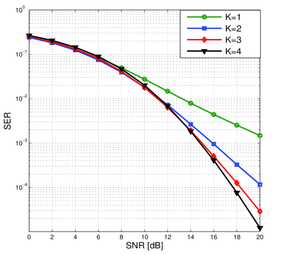
Figure 6: Multiple relay selection under outdated CSI when $N=4$, $K=1,2,3,4$, and $f_{d}T_{d}=0.1$.

Fig. 6 studies the performance of multiple RS when $N=4$ and $f_{d}T_{d}=0.1$. The best $K$ relays, $K=1,2,3,4$, are selected according to (27) and the maximal ratio combining is adopted. For the sake of fairness, the total power of the selected relays is assumed to be the same, regardless of $K$. In addition, the total power is allocated equally among the selected relays, i.e, $p_{r}=P_{0}/K$. We also assume that $p_{s}=P_{0}$, and the x-axis of this figure is $\mbox{SNR}=P_{0}/\sigma_{n}^{2}$ in dB. From this figure, we find that in low SNR, the SER performance for different $K$ is almost the same, because the performance in low SNR is power-limited, and the total power is the same for different $K$. However, in high SNR, increasing the number of selected relays $K$ will significantly improve the SER performance, because the diversity order is $K$ with outdated CSI, which satisfies the analysis of Proposition 3. Therefore, multiple RS is a feasible solution to improve the diversity loss caused by the outdated CSI.

V Conclusions

The effect of outdated CSI on the SER performance of bidirectional AF RS has been investigated in this paper. For the single RS, the distribution of end-to-end SNR, the analytical and asymptotic expressions of SER are derived in a closed form, and verified by simulations. The effect of the number of relays and the correlation coefficient of outdated CSI are investigated. The results reveal that the SER performance of bidirectional RS is highly dependent on the outdated CSI. Specifically, the diversity order reduces to one from full diversity, once CSI is outdated. Furthermore, a multiple RS scheme is proposed, and the diversity order with outdated CSI is analyzed, which proves that the multiple RS scheme can compensate the diversity loss caused by outdated CSI.

Appendix A: Proof of Lemma 1

According to the inequality[7] ${xy}/{\left(x+y\right)}\leq\min\left(x,y\right),x,y>0$, we have

$$\min\left({\gamma_{1i},\gamma_{2i}}\right)\leq\min\left[{\min\left({\psi_{r}\left|{h_{1i}}\right|^{2},\psi_{h}\left|{h_{2i}}\right|^{2}}\right),\min\left({\psi_{h}\left|{h_{1i}}\right|^{2},\psi_{r}\left|{h_{2i}}\right|^{2}}\right)}\right].$$ (29)

Furthermore, by the fact $\psi_{r}>\psi_{h}\buildrel\Delta\over{=}{\psi_{r}\psi_{s}}/\left({\psi_{r}+\psi_{s}}\right)$ and discussion under different conditions, we will verify that

$$\min\left[{\min\left({\psi_{r}\left|{h_{1i}}\right|^{2},\psi_{h}\left|{h_{2i}}\right|^{2}}\right),\min\left({\psi_{h}\left|{h_{1i}}\right|^{2},\psi_{r}\left|{h_{2i}}\right|^{2}}\right)}\right]=\psi_{h}\min\left({\left|{h_{1i}}\right|^{2},\left|{h_{2i}}\right|^{2}}\right).$$ (30)

The process of verifying (30) is listed as follows, where $\psi_{h}<\psi_{r}$:

(i) If $\psi_{r}|h_{1i}|^{2}<\psi_{h}|h_{2i}|^{2}$, we have $|h_{1i}|^{2}<|h_{2i}|^{2}$, thus $\psi_{h}|h_{1i}|^{2}<\psi_{r}|h_{2i}|^{2}$. Therefore, we have

$$I\buildrel\Delta\over{=}\min\left[{\min\left({\psi_{r}|h_{1i}|^{2},\psi_{h}|h_{2i}|^{2}}\right),\min\left({\psi_{h}|h_{1i}|^{2},\psi_{r}|h_{2i}|^{2}}\right)}\right]$$

$$=\min\left({\psi_{r}|h_{1i}|^{2},\psi_{h}|h_{1i}|^{2}}\right)=\psi_{h}|h_{1i}|^{2}=\psi_{h}\min\left({|h_{1i}|^{2},|h_{2i}|^{2}}\right)$$ (31)

(ii) If $\psi_{r}|h_{1i}|^{2}\geq\psi_{h}|h_{2i}|^{2}$, $\min\{\psi_{r}|h_{1i}|^{2},\psi_{h}|h_{2i}|^{2}\}=\psi_{h}|h_{2i}|^{2}$.

(iia) Under situation (ii) and if $\psi_{h}|h_{1i}|^{2}<\psi_{r}|h_{2i}|^{2}$, we have $\min\{\psi_{h}|h_{1i}|^{2},\psi_{r}|h_{2i}|^{2}\}=\psi_{h}|h_{1i}|^{2}$, thus

$$I=\psi_{h}\min\left({|h_{1i}|^{2},|h_{2i}|^{2}}\right).$$ (32)

(iib) Under situation (ii) and if $\psi_{h}|h_{1i}|^{2}\geq\psi_{r}|h_{2i}|^{2}$, we have $\min\{\psi_{h}|h_{1i}|^{2},\psi_{r}|h_{2i}|^{2}\}=\psi_{r}|h_{2i}|^{2}$ and $|h_{1i}|^{2}>|h_{2i}|^{2}$, thus

$$I=\min\left({\psi_{h}|h_{2i}|^{2},\psi_{r}|h_{2i}|^{2}}\right)=\psi_{h}|h_{2i}|^{2}=\psi_{h}\min\left({|h_{1i}|^{2},|h_{2i}|^{2}}\right).$$ (33)

In summary of (Appendix A: Proof of Lemma 1), (32), and (33), (30) is achieved. Therefore, Lemma 1 is verified according to (29) and (30).

Appendix B: Proof of Lemma 2

Inspired by [10], the PDF of $|h_{1k}|^{2}$ can be expanded as

$$f_{\left|{h_{1k}}\right|^{2}}\left(z\right)\buildrel(a)\over{=}\frac{d}{{dz}}\sum\limits_{i=1}^{N}{\Pr\left\{{\left|{h_{1i}}\right|^{2}<z\cap k=i}\right\}}$$

$$=\frac{d}{{dz}}\sum\limits_{i=1}^{N}{\int\limits_{0}^{z}{\int\limits_{0}^{\infty}{f_{\left|{h_{1i}}\right|^{2},\left|{\hat{h}_{1i}}\right|^{2}}\left({x,y}\right)}}\Pr\left\{{k=i|\left|{h_{1i}}\right|^{2}=x,\left|{\hat{h}_{1i}}\right|^{2}=y}\right\}dxdy}$$

$$=\sum\limits_{i=1}^{N}{\int\limits_{0}^{\infty}{f_{\left|{h_{1i}}\right|^{2}|\left|{\hat{h}_{1i}}\right|^{2}}\left({z|y}\right)f_{\left|{\hat{h}_{1i}}\right|^{2}}\left(y\right)\Pr\left\{{k=i|{\left|{\hat{h}_{1i}}\right|^{2}}=y}\right\}dy}}$$

$$\buildrel(b)\over{=}\sum\limits_{i=1}^{N}{\int\limits_{0}^{\infty}{f_{\left|{h_{1i}}\right|^{2}|\left|{\hat{h}_{1i}}\right|^{2}}\left({z|y}\right)f_{\left|{\hat{h}_{1i}}\right|^{2}}\left(y\right)\Pr\left\{{\left|{\hat{h}_{1i}}\right|^{2}\leq\left|{\hat{h}_{2i}}\right|^{2}|\left|{\hat{h}_{1i}}\right|^{2}=y}\right\}\Pr\left\{{k=i|\left|{\hat{h}_{1i}}\right|^{2}=y,\left|{\hat{h}_{1i}}\right|^{2}\leq\left|{\hat{h}_{2i}}\right|^{2}}\right\}dy}}$$

$$+\sum\limits_{i=1}^{N}{\int\limits_{0}^{\infty}{f_{\left|{\hat{h}_{1i}}\right|^{2}|\left|{\hat{h}_{2i}}\right|^{2}}\left({z|y}\right)f_{\left|{\hat{h}_{1i}}\right|^{2}}\left(y\right)\Pr\left\{{\left|{\hat{h}_{1i}}\right|^{2}>\left|{\hat{h}_{2i}}\right|^{2}|\left|{\hat{h}_{1i}}\right|^{2}=y}\right\}\Pr\left\{{k=i|\left|{\hat{h}_{1i}}\right|^{2}=y,\left|{\hat{h}_{1i}}\right|^{2}>\left|{\hat{h}_{2i}}\right|^{2}}\right\}dy}}$$

$$\buildrel(c)\over{=}\sum\limits_{i=1}^{N}{\int\limits_{0}^{\infty}{f_{\left|{h_{1i}}\right|^{2}\left|{\hat{h}_{1i}}\right|^{2}}\left({z|y}\right)f_{\left|{\hat{h}_{1i}}\right|^{2}}\left(y\right)\Pr\left\{{\left|{\hat{h}_{1i}}\right|^{2}\leq\left|{\hat{h}_{2i}}\right|^{2}|\left|{\hat{h}_{1i}}\right|^{2}=y}\right\}I_{i}\left(y\right)dy}}$$

$$+\sum\limits_{i=1}^{N}{\int\limits_{0}^{\infty}{f_{\left|{h_{1i}}\right|^{2}|\left|{\hat{h}_{1i}}\right|^{2}}\left({z|y}\right)f_{\left|{\hat{h}_{1i}}\right|^{2}}\left(y\right)\Pr\left\{{\left|{\hat{h}_{1i}}\right|^{2}>\left|{\hat{h}_{2i}}\right|^{2}|\left|{\hat{h}_{1i}}\right|^{2}=y}\right\}I_{i}\left({\left|{\hat{h}_{2i}}\right|^{2}}\right)dy}}$$ (34)

where (a) is satisfied by total probability theorem[24], in which the universal set $|h_{1k}|^{2}<z$ is divided into $N$ disjoint sets $|h_{1i}|^{2}<z$, $i=1,\ldots,N$; (b) is fulfilled by the division of two disjoint events, i.e., $|\hat{h}_{1i}|^{2}>|\hat{h}_{2i}|^{2}$ and $|\hat{h}_{1i}|^{2}\leq|\hat{h}_{2i}|^{2}$, and (c) is decided by the RS scheme (7), in which $I_{i}\left(x\right)\buildrel\Delta\over{=}\prod\limits_{q=1,q\neq i}^{N}{\Pr\left\{{\min\left(|\hat{h}_{1i}|^{2},|\hat{h}_{2i}|^{2}\right)\leq x}\right\}}$.

According to order statistics[25] and[19, eq. (26)] , $I_{i}\left(x\right)$ can be expanded as

$$I_{i}\left(x\right) =\prod\limits_{q=1,q\neq i}^{N}{\left\{{1-\left[{1-\Pr\left({|\hat{h}_{1q}|^{2}\leq x}\right)}\right]\left[{1-\Pr\left({|\hat{h}_{2q}|^{2}\leq x}\right)}\right]}\right\}}$$

$$=\prod\limits_{q=1,q\neq i}^{N}{\left\{{1-\exp\left({-\frac{x}{{\sigma_{q}^{2}}}}\right)}\right\}}$$

$$=1+\sum\limits_{t=1}^{N-1}{\sum\limits_{\scriptstyle A_{t}\subseteq\left\{{1,\ldots,N}\right\}\backslash i\hfill\atop\scriptstyle\left|{A_{t}}\right|=t\hfill}{\left({-1}\right)^{t}\exp\left({-x\sum\limits_{l\in A_{t}}{\frac{1}{{\sigma_{l}^{2}}}}}\right)}}$$ (35)

where $\frac{1}{{\sigma_{l}^{2}}}\buildrel\Delta\over{=}\frac{1}{{\sigma_{1l}^{2}}}+\frac{1}{{\sigma_{2l}^{2}}}$, $l=1,\ldots,N$.

According to the exponential distribution of $|\hat{h}_{1i}|^{2}$ and $|\hat{h}_{2i}|^{2}$, and the conditional PDF [10, eq. (31)]

$$f_{|h_{ji}|^{2}||\hat{h}_{ji}|^{2}}\left({z|y}\right)=\frac{1}{{\left({1-\rho_{ji}^{2}}\right)\sigma_{ji}^{2}}}\exp\left({-\frac{{\rho_{ji}^{2}y+z}}{{\left({1-\rho_{ji}^{2}}\right)\sigma_{ji}^{2}}}}\right)I_{0}\left({\frac{{2\sqrt{\rho_{ji}^{2}yz}}}{{\left({1-\rho_{ji}^{2}}\right)\sigma_{ji}^{2}}}}\right),$$ (36)

the PDF of $|h_{1k}|^{2}$ is verified by [23, eq. (6.614.3)]

$$\int_{0}^{\infty}{\exp\left(-\alpha x\right)I_{0}\left(\beta\sqrt{x}\right)}dx=\left({1}/{\alpha}\right)\exp\left({{\beta^{2}}}/\left({{4\alpha}}\right)\right),$$ (37)

and the PDF of $|h_{2k}|^{2}$ can be verified similarly.

Appendix C: Proof of Lemma 3

According to the fact [19, eq. (26)], i.e.,

$$\prod\limits_{q=1,q\neq i}^{N}{\left\{{1-\exp\left({-\frac{x}{{\sigma_{q}^{2}}}}\right)}\right\}}{\rm{=}}\sum\limits_{t=0}^{N-1}{\sum\limits_{A_{t}}{\left({-1}\right)^{t}\exp\left({-x\sum\limits_{l\in A_{t}}{\frac{1}{{\sigma_{l}^{2}}}}}\right)}},$$ (38)

we have

$$\sum\limits_{i=1}^{N}{\frac{1}{{\sigma_{i}^{2}}}}\exp\left({-\frac{x}{{\sigma_{i}^{2}}}}\right)\prod\limits_{q=1,q\neq i}^{N}{\left\{{1-\exp\left({-\frac{x}{{\sigma_{q}^{2}}}}\right)}\right\}}=\sum\limits_{i=1}^{N}{\frac{1}{{\sigma_{i}^{2}}}}\sum\limits_{t=0}^{N-1}{\sum\limits_{A_{t}}{\left({-1}\right)^{t}\exp\left({-\sum\limits_{l\in A_{t}}{\frac{x}{{\sigma_{l}^{2}}}-\frac{x}{{\sigma_{i}^{2}}}}}\right)}}.$$ (39)

By integrating both sides of (39) from $0$ to $\infty$, the formula can be expressed as

$$\prod\limits_{i=1}^{N}{\left\{{1-\exp\left({-\frac{x}{{\sigma_{i}^{2}}}}\right)}\right\}}\bigg{|}_{0}^{\infty}=\sum\limits_{i=1}^{N}{\frac{1}{{\sigma_{i}^{2}}}}\sum\limits_{t=0}^{N-1}{\sum\limits_{A_{t}}{\left({-1}\right)^{t}\frac{{\exp\left({-\sum\limits_{l\in A_{t}}{\frac{x}{{\sigma_{l}^{2}}}-\frac{x}{{\sigma_{i}^{2}}}}}\right)}}{{-\sum\limits_{l\in A_{t}}{\frac{1}{{\sigma_{l}^{2}}}-\frac{1}{{\sigma_{i}^{2}}}}}}}}\bigg{|}_{0}^{\infty}$$ (40)

where $f\left(x\right)\big{|}_{0}^{\infty}=f\left(\infty\right)-f\left(0\right)$, thus the first equation in Lemma 3 is proved.

Substituting $x$ with $0$ into (38), the second equation in Lemma 3 is proved when $k=0$.

Differentiating (38), we have

$$\sum\limits_{k=1,k\neq i}^{k=N}{\frac{1}{{\sigma_{k}^{2}}}}\prod\limits_{q=1,q\neq k,i}^{N}{\left\{{1-\exp\left({-\frac{x}{{\sigma_{q}^{2}}}}\right)}\right\}}=\sum\limits_{t=1}^{N-1}{\sum\limits_{A_{t}}{\left({\sum\limits_{l\in A_{t}}{\frac{\left({-1}\right)^{t+1}}{{\sigma_{l}^{2}}}}}\right)\exp\left({-\sum\limits_{l\in A_{t}}{\frac{x}{{\sigma_{l}^{2}}}}}\right)}},$$ (41)

then substituting $x$ with $0$, the second equation in Lemma 3 is proved when $k=1$.

It is easily verified that for $k=2,\ldots,N-2$, the second equation in Lemma 3 is achieved by differentiating (41) continually and then substituting $x$ with $0$ subsequently.

Appendix D: Proof of Proposition 1 and Proposition 2

The received SNR of $S_{1}$ is $\gamma_{1k}=\Omega_{1}\Omega_{2}/\left(\Omega_{1}+\Omega_{2}\right)$, where $\Omega_{1}=\psi_{r}|h_{1k}|^{2}$ and $\Omega_{2}=\psi_{h}|h_{2k}|^{2}$. Therefore, the CDF of $\gamma_{1k}$ can be written as

$$F_{\gamma_{1k}}\left(z\right) =\Pr\left\{{\frac{{\Omega_{1}\Omega_{2}}}{{\Omega_{1}+\Omega_{2}}}<z}\right\}$$

$$=\Pr\left\{{\left({\Omega_{2}-z}\right)\Omega_{1}<z\Omega_{2},\Omega_{2}>z}\right\}+\Pr\left\{{\left({\Omega_{2}-z}\right)\Omega_{1}<z\Omega_{2},\Omega_{2}\leq z}\right\}$$

$$=\int_{z}^{\infty}{F_{\Omega_{1}}\left({\frac{{zx}}{{x-z}}}\right)}f_{\Omega_{2}}\left(x\right)dx+\int_{0}^{z}{\left[{1-F_{\Omega_{1}}\left({\frac{{zx}}{{x-z}}}\right)}\right]}f_{\Omega_{2}}\left(x\right)dx$$

$$=1-\int\limits_{0}^{\infty}{f_{\Omega_{2}}\left({x+z}\right)\left[{1-F_{\Omega_{1}}\left({z+\frac{{z^{2}}}{x}}\right)}\right]}dx.$$ (42)

Substituting $\int\limits_{0}^{\infty}{\exp\left(-mx-nx^{-1}\right)}dx=2\sqrt{{n}/{m}}K_{1}\left(2\sqrt{mn}\right)$ [23, eq. (3.324)] into (Appendix D: Proof of Proposition 1 and Proposition 2), Proposition 1 can be proved by Lemma 2.

Applying Proposition 1 and (18), the exact average SER of $S_{1}$ can be obtained by [23, eq. (6.621.3)]

$$\int_{0}^{\infty}{x^{\mu-1}}e^{-\alpha x}K_{\nu}\left(\beta x\right)dx=\frac{{\sqrt{\pi}\left(2\beta\right)^{\nu}}}{{\left(\alpha+\beta\right)^{\mu+\nu}}}\frac{{\Gamma\left(\mu+\nu\right)\Gamma\left(\mu-\nu\right)}}{{\Gamma\left(\mu+1/2\right)}}F\left(\mu+\nu,\nu+\frac{1}{2};\mu+\frac{1}{2};\frac{{\alpha-\beta}}{{\alpha+\beta}}\right)$$ (43)

where $\Gamma\left(\cdot\right)$ is the Gamma function, and $F\left(\cdot\right)$ is the Confluent Hypergeometric function[22].

The performance of $S_{2}$ can be verified similarly.

It is noted that the CSI of the selected path is also assumed to be perfect for data transmission, although the CSI used for relay selection is outdated. The reasoning behind this assumption lies in the fact that the time-repetition rates between the above two processes, i.e., relay selection and data transmission, are generally different [10]. We also assume that the channel reciprocity is satisfied, i.e., the channel stays constant during the two phases of communication. This assumption is reasonable, when the frame length of the two phases is relatively small, or the correlation coefficient of outdated CSI is relatively large. Furthermore, this assumption is also made in the previous research of two-way relay with outdated CSI, such as the user selection [14] and the antenna selection [15]. Therefore, we follow this assumption in this paper.

Appendix E: Proof of Corollary 1 and Corollary 2

In high SNR, i.e., $\psi_{s},\psi_{r}\to\infty$, we have $a_{i}\to 0$ and $b_{i}^{\prime}\to 0$. According to $xy/\big{(}x+y\big{)}\approx\min\big{(}x,y\big{)}$ and the order statistics[25], the CDF of $\gamma_{1k}$ is expressed as

$$F_{\gamma_{1k}}\left(z\right)=1-\left[{1-F_{\left|{h_{1k}}\right|^{2}}\left({\frac{z}{{\psi_{r}}}}\right)}\right]\left[{1-F_{\left|{h_{2k}}\right|^{2}}\left({\frac{z}{{\psi_{h}}}}\right)}\right]$$ (44)

where the CDF of $|h_{jk}|^{2}$ can be obtained by integrating (Appendix B: Proof of Lemma 2).

If CSI is perfect, i.e., $\rho_{ji}=1$, the CDF of $\psi_{r}|h_{1k}|^{2}$ is expanded as

$$F_{\left|{h_{1k}}\right|^{2}}\left(\frac{z}{\psi_{r}}\right)\buildrel(a)\over{=}-\sum\limits_{p=1}^{\infty}{\frac{{\left({-1}\right)^{p}}}{{p!}}\left({\frac{z}{{\psi_{r}\sigma_{1i}^{2}}}}\right)^{p}\sum\limits_{i=1}^{N}{\sum\limits_{t=0}^{N-1}{\sum\limits_{A_{t}}{\left({-1}\right)^{t}}}}\frac{{1+\left({\sum\limits_{j\in A_{t}}{\frac{{\sigma_{2i}^{2}}}{{\sigma_{j}^{2}}}}}\right)\left({\frac{{\sigma_{1i}^{2}}}{{\sigma_{i}^{2}}}+\sum\limits_{j\in A_{t}}{\frac{{\sigma_{1i}^{2}}}{{\sigma_{j}^{2}}}}}\right)^{p-1}}}{{1+\sum\limits_{j\in A_{t}}{\frac{{\sigma_{2i}^{2}}}{{\sigma_{j}^{2}}}}}}}$$

$$\buildrel(b)\over{=}-\sum\limits_{p=1}^{\infty}{\frac{{\left({-1}\right)^{p}}}{{p!}}\left({\frac{z}{{\psi_{r}\sigma_{1i}^{2}}}}\right)^{p}\sum\limits_{i=1}^{N}{\sum\limits_{t=0}^{N-1}{\sum\limits_{A_{t}}{\left({-1}\right)^{t}}}}}\left({\sum\limits_{j\in A_{t}}{\frac{{\sigma_{2i}^{2}}}{{\sigma_{j}^{2}}}}}\right)\sum\limits_{k=1}^{p-1}{\binom{p-1}{k}\left({\frac{{\sigma_{1i}^{2}}}{{\sigma_{2i}^{2}}}}\right)}^{k}\left({1+\sum\limits_{j\in A_{t}}{\frac{{\sigma_{2i}^{2}}}{{\sigma_{j}^{2}}}}}\right)^{k-1}$$

$$\buildrel(c)\over{=}-\sum\limits_{p=1}^{\infty}{\frac{{\left({-1}\right)^{p}}}{{p!}}\left({\frac{z}{{\psi_{r}\sigma_{1i}^{2}}}}\right)^{p}\sum\limits_{i=1}^{N}{\sum\limits_{t=0}^{N-1}{\sum\limits_{A_{t}}{\left({-1}\right)^{t}}}}}\sum\limits_{k=1}^{p-1}{\binom{p-1}{k}\left({\frac{{\sigma_{1i}^{2}}}{{\sigma_{2i}^{2}}}}\right)}^{k}\sum\limits_{q=0}^{k-1}{\binom{k-1}{q}}\left({\sum\limits_{j\in A_{t}}{\frac{{\sigma_{2i}^{2}}}{{\sigma_{j}^{2}}}}}\right)^{q+1}$$

$$\buildrel(d)\over{\approx}-\frac{{\left({-1}\right)^{N}}}{{N!}}\left({\frac{z}{{\psi_{r}\sigma_{1i}^{2}}}}\right)^{N}\sum\limits_{i=1}^{N}{\sum\limits_{t=0}^{N-1}{\sum\limits_{A_{t}}{\left({-1}\right)^{t}}}}\left({\sum\limits_{j\in A_{t}}{\frac{{\sigma_{1i}^{2}}}{{\sigma_{j}^{2}}}}}\right)^{N-1}$$ (45)

where (a) is satisfied by the Macraulian series $\exp\left(x\right)=\sum\limits_{p=0}^{\infty}x^{p}/p!$ and the first equation in Lemma 3; (b) is fulfilled by the binomial expansion of $\big{[}{\frac{{\sigma_{1i}^{2}}}{{\sigma_{i}^{2}}}+\sum\limits_{j\in A_{t}}{\frac{{\sigma_{1i}^{2}}}{{\sigma_{j}^{2}}}}}\big{]}^{p-1}=\bigg{[}{1+\frac{{\sigma_{1i}^{2}}}{{\sigma_{2i}^{2}}}\big{(}{1+\sum\limits_{j\in A_{t}}{\frac{{\sigma_{2i}^{2}}}{{\sigma_{j}^{2}}}}}\big{)}}\bigg{]}^{p-1}$ and the second equation in Lemma 3; (c) is achieved by the binomial expansion of $\big{(}{1+\sum\limits_{j\in A_{t}}{\frac{{\sigma_{2i}^{2}}}{{\sigma_{j}^{2}}}}}\big{)}^{k-1}$; (d) is obtained also by the second equation in Lemma 3, and ignoring the high order infinitesimal.

The CDF of $\psi_{h}|h_{2k}|^{2}$ can be obtained similarly, thus the asymptotic SER of $S_{1}$ with perfect CSI can be achieved by (44), (18), and $\int_{0}^{\infty}{t^{2N}}\exp\left(-{t^{2}}/{2}\right)dt={2^{\left(N-{1}/{2}\right)}}\Gamma\left({1}/{2}+N\right)$ in [23, eq. (3.326.2)], where $\Gamma\left(\cdot\right)$ is the Gamma function[22]. Therefore, the diversity order is $N$.

If CSI is outdated, applying Macraulian series $\exp\left(x\right)\approx 1+x$, the CDF of $\psi_{r}|\hat{h}_{1k}|^{2}$ can be written as

$$F_{{\left|{h_{1k}}\right|^{2}}}\left(\frac{z}{\psi_{r}}\right)\approx\sum\limits_{i=1}^{N}{\sum\limits_{t=0}^{N-1}{\sum\limits_{A_{t}}{\left({-1}\right)^{t}}}}\frac{{1+\zeta_{1}}}{{1+\sum\limits_{l\in A_{t}}{\frac{{\sigma_{2i}^{2}}}{{\sigma_{l}^{2}}}}}}\frac{z}{{\psi_{r}\sigma_{1i}^{2}}}$$ (46)

where the high order infinitesimal is ignored.

The CDF of $\psi_{h}|h_{2k}|^{2}$ can be obtained similarly, thus the asymptotic SER of $S_{1}$ with outdated CSI can be achieved by (44), (18), and $\int_{0}^{\infty}{t^{2N}}\exp\left(-{t^{2}}/{2}\right)dt={2^{\left(N-{1}/{2}\right)}}\Gamma\left({1}/{2}+N\right)$ in [23, eq. (3.326.2)]. Therefore, the diversity order is $1$.

The asymptotic expressions of $S_{2}$ can be verified similarly.

It is noted that although the analytical expression in Proposition 2 is the lower bound, it matches tightly with the exact result, especially in high SNR. Furthermore, diversity order reflects the behavior of SER in high SNR. Therefore, similar to the previous research [4], the diversity analysis, obtained by the analytical expression, is accurate.

Another alternative method to analyze the diversity is achieved by the SNR bounds. The end-to-end instantaneous SNR is upper bounded by $\min\{\psi_{r}|h_{ji}|^{2},\psi_{h}|h_{\bar{j}i}|^{2}\}$, and lower bounded by $\frac{1}{2}\min\{\psi_{s}|h_{ji}|^{2},\psi_{h}|h_{\bar{j}i}|^{2}\}$. Similar to the previous analysis, the diversity order can also be obtained.

Appendix F: Proof of Proposition 3

For ease of analysis, the performance of diversity order is obtained under the symmetric network, i.e., $\sigma_{ji}^{2}=1$ and $\rho_{ji}=\rho$.

According to Lemma 1, we have the asymptotic performance

$$\gamma_{i}=\min\big{(}\gamma_{1i},\gamma_{2i}\big{)}\approx\psi_{h}\min\big{(}|h_{1i}|^{2},|h_{2i}|^{2}\big{)}.$$ (47)

Therefore, $\gamma_{i}$ follows the exponential distribution, i.e.,

$$f_{\gamma_{i}}\big{(}x\big{)}=\frac{1}{\Gamma}\exp\big{(}-\frac{x}{\Gamma}\big{)}$$ (48)

where $\Gamma=\psi_{h}/2$.

Denoting $\hat{\gamma}_{i}$ to be the outdated version of $\gamma_{i}$, the received SNR by maximal-ratio combining the best $K$ relays is

$$\gamma=\sum\limits_{i=0}^{N}T(\hat{\gamma}_{i})$$ (49)

where $T(\hat{\gamma}_{i})$ indicates whether $R_{i}$ is selected or not, according to the RS scheme (7), i.e.,

$$T\left({\hat{\gamma}_{i}}\right)=\left\{{\begin{array}[]{*{20}c}{0,\hat{\gamma}_{i}<\hat{\gamma}^{\left(K\right)};\hfill}\\ {\gamma_{i},\hat{\gamma}_{i}\geq\hat{\gamma}^{\left(K\right)}.\hfill}\\ \end{array}}\right.$$ (52)

where $\hat{\gamma}^{\left(K\right)}$ represents the $K$th largest value among $\left\{\hat{\gamma}_{i}|i=1,\ldots,N\right\}$.

Following the analysis of [13], the moment generating function (MGF) of $\gamma$ in (49) is obtained by dividing the total probability into $N$ disjoint events that $\hat{\gamma}_{i}=\hat{\gamma}^{\left(K\right)},i=1,\ldots,N$. During each event, there are $\big{(}K-1\big{)}$ relays whose SNR is larger than $\hat{\gamma}_{i}$, and other $\big{(}N-K\big{)}$ relays’ SNR is smaller than $\hat{\gamma}_{i}$, thus there are $\binom{N-1}{K-1}$ possibilities.

After some manipulation, the MGF of $\gamma$ in (49) for the symmetric network is [13, eq. (15)]

$$\Phi_{\gamma}\left(s\right)=N\binom{N-1}{K-1}\sum\limits_{n=0}^{N-K}{\sum\limits_{q=0}^{N-K-n}{\sum\limits_{m=0}^{n}{\left({\frac{4}{-s\psi_{h}}}\right)}}}^{N-n}$$

$$\hskip 113.81102pt\times\frac{{\left({N-K}\right)!\left({-1}\right)^{q+m}}}{{\left({N-K-n-q}\right)!m!q!\left({n-m}\right)!}}\frac{1}{N-n+m-m\rho^{2}}.$$ (53)

Therefore, the diversity order is $K$, according to [21, prop. 3].

Figure 5: Diversity order versus finite SNR under different $f_{d}T_{d}$ and different $N$.

References

- [1] S. Zhang and S.-C. Liew, “Channel coding and decoding in a relay system operated with physical-layer network coding,” IEEE J. Sel. Areas in Commun., vol. 27, no. 5, pp.788–796, Jun. 2009.
- [2] R. H. Y. Louie, Y. Li, and B. Vucetic, “Practical physical layer network coding for two-way relay channels: Performance analysis and comparison,” IEEE Trans. Wireless Commun., vol. 9, no. 2, pp. 764–777, Feb. 2010.
- [3] P. Popovski and H. Yomo, “Wireless network coding by amplify-and-forward for bi-directional traffic flows,” IEEE Commun. Lett., vol. 11, no. 1, pp. 16–18, Jan. 2007.
- [4] L. Song, “Relay selection for two-way relaying with amplify-and-forward protocols,” IEEE Trans. Veh. Technol., vol. 60, no. 4, pp. 1954–1959, May 2011.
- [5] Y. Jing, “A relay selection scheme for two-way amplify-and-forward relay networks,” in Proc. Inter. Conf. Wireless Commun. Signal Process., Nov. 2009.
- [6] K. Hwang, Y. Ko, and M.-S. Alouini, “Performance bounds for two-way amplify-and-forward relaying based on relay path selection,” in Proc. Veh. Technol. Conf., Apr. 2009.
- [7] P. K. Upadhyay and S. Prakriya, “Performance of two-way opportunistic relaying with analog network coding over Nakagami-m fading,” IEEE Trans. Veh. Technol., vol. 60, no. 4, pp. 1965–1971, May 2011.
- [8] Y. Liu, M. Tao, B. Li, and H. Shen, “Optimization framework and graph-based approach for relay-assisted bidirectional OFDMA cellular networks,” IEEE Trans. Wireless Commun., vol. 9, no. 11, pp. 3490–3500, Nov. 2010.
- [9] H. X. Nguyen, H. H. Nguyen, and T. Le-Ngoc, “Diversity analysis of relay selection schemes for two-way wireless relay networks,” Wireless Pers. Commun., Jan. 2010.
- [10] D. S. Michalopoulos, H. A. Suraweera, G. K. Karagiannidis, and R. Schober, “Amplify-and-forward relay selection with outdated channel estimates,” IEEE Trans. Commun., Dec. 2010. vol. 60, no. 5, pp. 1278–1290, May 2012.
- [11] M. Soysa, H. Suraweera, C. Tellambura, and H. Garg, “Partial and opportunistic relay selection with outdated channel estimates,” IEEE Trans. Commun., vol. 60, no. 3, pp. 840–850, Mar. 2012.
- [12] M. Seyfi, S. Muhaidat, J. Liang, and M. Dianati, “Effect of feedback delay on the performance of cooperative networks with relay selection,” IEEE Trans. Wireless Commun., vol. 10, no. 12, pp. 4161–4171, Dec. 2011.
- [13] M. Chen, T. C.-K. Liu, and X. Dong, “Opportunistic multiple relay selection with outdated channel state information,” IEEE Trans. Veh. Technol., vol. 61, no. 3, pp. 1333–1345, Mar. 2012.
- [14] L. Fan, X. Lei, P. Fan, and R. Q. Hu, ”Outage probability analysis and power allocation for two-way relay networks with user selection and outdated channel state information,” IEEE Commun. Lett. , vol. 16, no. 5, pp. 638–641, May 2012.
- [15] G. Amarasuriya, C. Tellambura, and M. Ardakani, “Two-way amplify-and-forward multiple-input multiple-output relay networks with antenna selection,” IEEE J. Sel. Areas Commun., vol. 30, no. 8, pp. 1513–1529, Sep. 2012.
- [16] A. Bletsas, A. Khisti, D. P. Reed, and A. Lippman, “A simple cooperative diversity method based on network path selection,” IEEE J. Sel. Areas Commun., vol. 24, no. 3, pp. 659–672, Mar. 2006.
- [17] Y. Li, Q. Yin, W. Xu, H. Wang, “On the design of relay selection strategies in regenerative cooperative networks with outdated CSI,” IEEE Trans. Wireless Commun., vol. 10, no. 9, pp. 3086–3097, Sep. 2011.
- [18] F. Gao, R. Zhang, and Y. Liang, “Optimal channel estimation and training design for two-way relay networks,” IEEE Trans. Commun., vol. 57, no. 10, pp. 3024–3033, Oct. 2009.
- [19] H. Ding, J. Ge, D. B. Costa, and Z. Jiang , “A new efficient low-complexity scheme for multi-source multi-relay cooperative networks,” IEEE Trans. Veh. Technol., vol. 60, no. 2, pp. 716–722, Feb. 2011.
- [20] Y. Jing and H. Jafarkhani, “Single and multiple relay selection schemes and their achievable diversity orders,” IEEE Trans. Wireless Commun., vol. 8, no. 3, pp. 1414–1423, Mar. 2009.
- [21] Z. Wang and G. B. Giannakis, “A simple and general parameterization quantifying performance in fading channels,” IEEE Trans. Commun., vol. 51, no. 8, pp. 1389–1398, Aug. 2003.
- [22] M. Abramowitz and I. A. Stegun, Handbook of mathematical functions with formulas, graphs, and mathematical tables, 9th Edition, NewYork: Dover, 1970.
- [23] I. S. Gradshteyn and I. M. Ryzhik, Table of integals, series, and products, 5th Edition, Academic Press, 1994.
- [24] A. Paoulis and S. U. Pialli, Probability, random variables and stochastic processes, 4th Edition, McGraw-Hill, 2002.
- [25] H. A. David, Order statistics, Jonh Wiley Sons, Inc., 1970.