A statistical relation between the X-ray spectral index and Eddington ratio of active galactic nuclei in deep surveys

Abstract

We present an investigation into how well the properties of the accretion flow onto a supermassive black hole may be coupled to those of the overlying hot corona. To do so, we specifically measure the characteristic spectral index, $\Gamma$, of a power-law energy distribution, over an energy range of 2 to 10 keV, for X-ray selected, broad-lined radio-quiet active galactic nuclei (AGN) up to z$\sim$2 in COSMOS and E-CDF-S. We test the previously reported dependence between $\Gamma$ and black hole mass, FWHM and Eddington ratio using a sample of AGN covering a broad range in these parameters based on both the Mg ii and H$\alpha$ emission lines with the later afforded by recent near infrared spectroscopic observations using Subaru/FMOS. We calculate the Eddington ratios, $\lambda_{\rm Edd}$, for sources where a bolometric luminosity ($L_{\rm Bol}$) has been presented in the literature, based on SED fitting, or, for sources where these data do not exist, we calculate $L_{\rm Bol}$ using a bolometric correction to the X-ray luminosity, derived from a relationship between the bolometric correction, and $L_{\rm{X}}$/$L_{3000}$. From a sample of 69 X-ray bright sources ($>$ 250 counts), where $\Gamma$ can be measured with greatest precision, with an estimate of $L_{\rm Bol}$, we find a statistically significant correlation between $\Gamma$ and $\lambda_{\rm Edd}$, which is highly significant with a chance probability of 6.59$\times 10^{-8}$. A statistically significant correlation between $\Gamma$ and the FWHM of the optical lines is confirmed, but at lower significance than with $\lambda_{\rm Edd}$ indicating that $\lambda_{\rm Edd}$ is the key parameter driving conditions in the corona. Linear regression analysis reveals that $\Gamma=(0.32\pm 0.05)$log₁₀$\lambda_{\rm Edd}$$+(2.27\pm 0.06)$ and $\Gamma=(-0.69\pm 0.11)$log₁₀(FWHM/km s^-1)$+(4.44\pm 0.42)$. Our results on $\Gamma$-$\lambda_{\rm Edd}$ are in very good agreement with previous results. While the $\Gamma$-$\lambda_{\rm Edd}$ relationship means that X-ray spectroscopy may be used to estimate black hole accretion rate, considerable dispersion in the correlation does not make this viable for single sources, however could be valuable however for large X-ray spectral samples, such as those to be produced by eROSITA.

1 Introduction

X-ray emission from AGN is ubiquitous (Tananbaum et al., 1979), and is often used itself as an indicator of black hole accretion activity. The hard X-ray ($>2$ keV) spectrum takes the form of, at least to first order, a power-law, where the photon flux, $F_{\gamma}=AE^{-\Gamma}$ (photons cm^-2 s^-1). The X-ray emission is thought to be produced by the Compton up-scattering of seed optical/UV photons, produced by thermal emission from the accretion disc (Shakura & Sunyaev, 1973). This is believed to be done by hot electrons forming a corona in proximity to the disc (e.g. Sunyaev & Titarchuk, 1980). Investigations into the X-ray emission can yield important insights into the accretion process and constrain accretion models (e.g. Haardt & Maraschi, 1991, 1993). However, many details regarding this process remain unclear, for example the geometry of the corona, its heating and the energy transfer between the two phases.

The discovery of the intrinsic power-law index measured to be $\Gamma\sim 1.9$ was an important step in supporting the disc-corona model (Pounds et al., 1990; Nandra & Pounds, 1994), as previous results presenting lower values (e.g. Mushotzky, 1984; Turner & Pounds, 1989) were a challenge for these models. Subsequent studies have tried to pin down the parameters of the accretion which give rise to the physical conditions of the corona, such as the electron temperature, T_e and optical depth to electron scattering, $\tau_{\rm es}$, upon which $\Gamma$ depends (Rybicki & Lightman, 1986).

The temperature, and thus emission spectrum of a standard Shakura & Sunyaev accretion disc depends on the mass accretion rate, $\dot{m}$, (Shakura & Sunyaev, 1973). The luminosity of the system is thus related to $\dot{m}$ via the accretion efficiency, $L_{\rm Bol}=\eta\dot{m}c^{2}$, which is often parametrised as a fraction of the Eddington luminosity, $L_{\rm Edd}$, by the Eddington ratio, $\lambda_{\rm Edd}$=$L_{\rm Bol}/L_{\rm Edd}$. $L_{\rm Edd}$ is the theoretical maximal luminosity achieved via accretion when accounting for radiation pressure and is dependent on the black hole mass ($L_{\rm Edd}=4\pi$ G$M_{\rm BH}$ $m_{\rm p}c/\sigma_{\rm T}\simeq 1.26\times 10^{38}$$M_{\rm BH}$  erg s^-1, where $M_{\rm BH}$ is the black hole mass in solar masses). Due to the dependance of the accretion disc spectrum on these parameters, several works have investigated how the coronal X-ray emission is coupled. It has been shown that $\Gamma$ is well correlated with the full width at half maximum (FWHM) of the broad optical emission lines, specifically H$\beta$ (e.g. Boller et al., 1996; Brandt et al., 1997), giving some indication that the gravitational potential, i.e. black hole mass, is key. Subsequently $\lambda_{\rm Edd}$ was shown to be strongly correlated with $\Gamma$ (Lu & Yu, 1999; Wang et al., 2004; Shemmer et al., 2006). However a known degeneracy exists between the H$\beta$ FWHM and $\lambda_{\rm Edd}$ of the system (Boroson & Green, 1992), making it difficult to determine the fundamental parameter behind these relationships. Shemmer et al. (2006)(S06) were able to break this degeneracy by adding highly luminous quasars to their analysis, concluding that $\lambda_{\rm Edd}$ is the primary parameter driving the conditions in the corona, giving rise to $\Gamma$. Shemmer et al. (2008) (S08) followed up the work of S06 by adding further luminous quasars, increasing the significance of the previous result.

Follow up studies have confirmed this relationship using larger samples and extending the range of parameters probed (e.g. Risaliti et al., 2009; Jin et al., 2012; Fanali et al., 2013). Furthermore, works into the possible dependence of $\Gamma$ on X-ray luminosity ($L_{\rm{X}}$) have reported a positive correlation between these quantities in high redshift sources (Dai et al., 2004; Saez et al., 2008), but not seen in the local universe (George et al., 2000; Brightman & Nandra, 2011), and an evolution of this correlation was also reported in Saez et al. (2008). One interpretation of this correlation, however, was that it is driven fundamentally by changes in $\dot{m}$. It has been shown that $\dot{m}$ can also be estimated from X-ray variability analysis (e.g. McHardy et al., 2006), where $\dot{m}$ is correlated with the break timescale in the power density spectrum. Papadakis et al. (2009) used this result when conducting a joint X-ray spectral and timing analysis of nearby Seyfert galaxies to show in an independent manner that $\Gamma$ correlates with $\dot{m}$. Furthermore, in a study of the X-ray variability in primarily local AGN, Ponti et al. (2012) find a significant correlation between the excess variance, $\sigma^{2}_{\rm rms}$, and $\Gamma$, which when considering the correlation between $\sigma^{2}_{\rm rms}$ and $\dot{m}$ that they find, is indirect evidence for the dependance of $\Gamma$ on $\dot{m}$.

The strong correlation between $\Gamma$ and accretion rate is interpreted as enhanced emission from the accretion disc in higher accretion rate systems more effectively cooling the corona, leading to a steepening of the X-ray emission (Pounds et al., 1995).

Not only is the $\Gamma$-$\lambda_{\rm Edd}$ correlation significant with respect to constraining accretion models, but as pointed out by S06, it allows an independent measurement of the black hole growth activity in galaxies from X-ray spectroscopy alone, and with a measurement of the bolometric luminosity, a black hole mass can be determined. This would be especially useful for moderately obscured AGN, where virial black hole mass estimates are not possible, but X-rays can penetrate the obscuration.

The aim of this work is to extend previous analyses on correlations with $\Gamma$ for the first time to the deep extragalactic surveys and in doing so, extending the range of parameters explored, breaking degeneracies between parameters where possible. By the use of survey data, we benefit from uniform X-ray data, where previous studies have relied on non-uniform archival data. In order to use $\Gamma$ as an Eddington ratio indicator, the dispersion in the relationship must be well parametrised, which we aim to do with the large range in parameters explored and our uniform X-ray coverage.

In addition, our black hole mass estimates are based on two optical lines, H$\alpha$ and Mg ii. Risaliti et al. (2009) (R09) showed that there was a stronger correlation with $\lambda_{\rm Edd}$ for measurements made with H$\beta$ compared to Mg ii and C iv, suggesting that this line is the best black hole mass indicator of the three. The H$\alpha$ data used here were specifically pursued partly in order to investigate the $\Gamma$ correlations with H$\alpha$ data for the first time at high redshifts, facilitated by near-infrared (NIR) spectroscopy. The parameters we explore in this work are $L_{\rm UV}$, $L_{\rm{X}}$, FWHM, $M_{\rm BH}$ and $\lambda_{\rm Edd}$.

In this work we assume a flat cosmological model with $H_{\rm 0}$=70 km s^-1 Mpc^-1 and $\Omega_{\Lambda}$=0.70. For measurement uncertainties on our spectral fit parameters we present the 90% confidence limits given two interesting parameters ($\Delta$c-stat=4.61).

2 Sample properties and data analysis

2.1 Sample selection

Our sample is based on two major extragalactic surveys, the extended Chandra Deep Field-South (E-CDF-S Lehmer et al., 2005), inclusive of the ultra-deep central area (Giacconi et al., 2002; Luo et al., 2008; Xue et al., 2011), and COSMOS surveys (Cappelluti et al., 2009; Elvis et al., 2009), where deep X-ray coverage with high optical spectroscopic completeness exists in both fields. The sample selection is as follows:

• We select sources with a black hole mass estimates based on H$\alpha$ or Mg ii from a black hole mass catalogue to be presented in Silverman, et al (in preparation). Mg ii line measurements were made from extensive existing optical spectra, primarily from zCOSMOS, Magellan/IMACS, Keck/Deimos and SDSS. Measurements of H$\alpha$ up to $z\sim 1.8$ are facilitated by the use of NIR spectroscopy from the Fiber Multi Object Spectrograph (FMOS) on the Subaru Telescope. The targets of these observations were Chandra X-ray selected AGN in COSMOS (Elvis et al., 2009) and E-CDF-S (Lehmer et al., 2005) with an already known spectroscopic redshift and detection of a broad emission line (FWHM$>$2000 km s^-1). A subset of the optical and NIR spectroscopic data analysis has already been presented in Matsuoka et al. (2013).

• In COSMOS we select Chandra sources also detected by XMM-Newton (see discussion in Brusa et al., 2010), due to the higher throughput capability of this observatory with respect to Chandra. For the E-CDF-S, we use the deep Chandra data available.

Combining these surveys and the selection criteria above yields a sample of 260 sources with both a black hole mass estimate and X-ray data, however, the main goal of this work is to investigate the detailed relationship between the coronal X-ray emission, characterised by the power-law index, $\Gamma$, and the parameters of the accretion, the observed quantities being luminosity and FWHM, and the derived quantities being $M_{\rm BH}$ and $\lambda_{\rm Edd}$. We therefore make the following cuts to the above sample as follows:

• We take sources where there are at least 250 source counts in the X-ray spectrum in order to get an accurate measurement of $\Gamma$. We describe this further in section 2.5.

• For analysis with $\lambda_{\rm Edd}$, a bolometric luminosity is required which we take from Lusso et al. (2012) (L12), which are derived from spectral energy distribution (SED) fitting. As these data do not exist for E-CDF-S sources, we use a bolometric correction to the X-ray luminosity, derived from $L_{\rm{X}}$/$L_{3000}$, which we describe in section 2.6. There are 44 which have an $L_{\rm Bol}$ from L12, all of which are in COSMOS, and 31 of which have $L_{\rm Bol}$ calculated using $L_{\rm{X}}$/$L_{3000}$, all of which are in the E-CDF-S.

• As we wish to study the properties of the coronal emission, responsible for the majority of X-ray emission in radio quiet AGN, we exclude radio loud sources. For this we make a cut of R$<$100, where R is the radio loudness parameter (Kellermann et al., 1989), excluding six sources. We describe the radio properties of our sample in section 2.7. Our final sample consists of 73 sources for analysis with FWHM and $M_{\rm BH}$ and 69 sources for analysis with $\lambda_{\rm Edd}$.

  Fig 1 shows how our final sample spans the redshift-luminosity plane, and how it compares to the sample of R09 which is derived from the SDSS/XMM-Newton quasar survey of Young et al. (2009). Our combination of wide and deep survey data allows us to span a larger luminosity range than done previously, and better sample to luminosity-redshift plane.

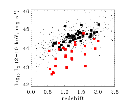
Figure 1: Plot of the redshift and X-ray luminosity distribution in our combined sample, where large red data points are from the E-CDF-S and the large black data points are from COSMOS. The sample covers redshifts up to $\sim 2.1$ and 2-10 keV X-ray luminosities of $42.5\lesssim$ log$L_{\rm X}$/erg s${}^{-1}\lesssim 45.5$. The dots show the sample of R09, which is derived from the SDSS/XMM-Newton quasar survey of Young, et al (2009).

2.2 Emission line measurements and black hole mass estimation

The first step in our analysis is to determine the accretion parameters, the velocity dispersion of the material around the black hole, characterised by the FWHM of the optical lines and $M_{\rm BH}$, which we derive from single-epoch optical spectral line fitting. A full description of the target selection, data analysis, including spectral line fitting, and results on virial black hole mass is presented in Matsuoka et al. (2013), which we briefly describe here.

Mg ii line measurements were made from optical spectra obtained primarily from zCOSMOS, Magellan/IMACS and SDSS. Fitting of the Mg ii line was carried out using a power-law to characterise the continuum, and one to two Gaussians used for the line. A broad Fe emission component is also included, which is based on the empirical template of Vestergaard & Wilkes (2001).

The H$\alpha$ measurements used here were the result of a campaign to make Balmer line observations of AGN outside the optical window at $z>0.8$ in the NIR with Subaru/FMOS. FMOS observations were made in low resolution mode ($\Delta\lambda/\lambda\simeq 600$) simultaneously in the J (1.05-1.34 ${\mu}$m) and H (1.43-1.77 ${\mu}$m) bands, yielding a velocity resolution of FWHM$\sim$500 km s^-1 at $\lambda=1.5$ ${\mu}$m. The target selection was such that the continuum around H$\alpha$ could be accurately determined and fit by a power-law. The H$\alpha$ line was fit by 2 to 3 Gaussians, while the neighbouring [NII]$\lambda$6548,6684 lines were fit with a pair of Gaussians.

Virial black hole estimates were calculated with the following formula:

$${\rm log}\frac{M_{\rm BH}}{M_{\odot}}=a+b\,{\rm log}\frac{\lambda L_{\lambda}\,\rm{or}\,L_{\rm line}}{10^{44}\mbox{\thinspace erg\thinspace s${}^{-1}$}}+c\,\rm{log}\frac{\rm FWHM}{\rm kms^{-1}}$$ (1)

where a=1.221, b=0.550 and c=2.060 for H$\alpha$ from Greene & Ho (2005) and a=0.505, b=0.620 and c=2.000 for Mg ii from McLure & Jarvis (2002). For H$\alpha$, the line luminosity is used in the calculation, whereas for Mg ii the monochromatic luminosity at 3000 Å is used.

In Matsuoka et al. (2013) a comparison of virial black hole mass estimates from H$\alpha$ and Mg ii is presented. They find a tight correlation between $L_{\rm H\alpha}$ and $L_{3000}$ and a close one-to-one relationship between the FWHM of H$\alpha$ and Mg ii, therefore leading to good agreements between the mass estimates from these lines. While H$\beta$ detections with FMOS do exist for this sample, measurements with this line is to be presented in a forthcoming publication (Silverman, et al. in preparation).

2.3 X-ray Data: Chandra Deep Field-South

In the E-CDF-S, the targets of the FMOS observations were the optical counterparts of type 1 AGN detected in the E-CDF-S survey described by Lehmer et al. (2005). The E-CDF-S consists of nine individual observations with four different central pointing positions, to a depth of 250 ks. The central region of the E-CDF-S survey is the location of the ultra deep 4 Ms E-CDF-S survey, which is described by Xue et al. (2011) and consists of 52 individual observations with a single central pointing position. We utilise all the Chandra data in this region. The data were screened for hot pixels and cosmic afterglows as described in Laird et al. (2009), astrometric corrections made as described in Rangel et al. (2013) and the source spectra were extracted using the acis extract (AE) software package (Broos et al., 2010), using the positions of the E-CDF-S sources. AE extracts spectral information for each source from each individual observation ID (obsID) based on the shape of the local point spread function (PSF) for that particular position on the detector. We choose to use regions where 90% of the PSF has been enclosed at 1.5 keV. Background spectra are extracted from an events list which has been masked of all detected point sources in Xue et al. (2011) and Lehmer et al. (2005), using regions which contain at least 100 counts. AE also constructs response matrix files (RMF) and auxiliary matrix files (ARF). The data from each obsID are then merged to create a single source spectrum, background spectrum, RMF and ARF for each source. The rest-frame 2-10 keV signal-to-noise ratios in this field range from 2.5 to 500.

2.4 X-ray Data: XMM-COSMOS

In the COSMOS survey, the targets of the FMOS observations were the optical counterparts of type 1 AGN detected in the Chandra-COSMOS survey (Elvis et al., 2009; Civano et al., 2012). However, as medium-depth ($\sim$60ks) XMM-Newton data exist in this field, we take advantage of the high throughput of this satellite to obtain X-ray spectral data. The XMM-COSMOS data are described in Cappelluti et al. (2009) and the procedure adopted to extract sources and background spectra in Mainieri et al. (2007). We briefly recall the main steps here. The task region of the XMM-Newton Science Analysis System (SAS) software has been used to generate the source and background extraction regions. The source region is defined as a circle with radius r_s that varies according to the signal-to-noise and the off-axis angle of the detection to optimise the quality of the final spectrum. The radii of these regions are reduced by the task to avoid overlapping with the extraction regions of nearby sources. All source regions are further excised from the area used for the background measurement. The task especget has been used to extract from the event file the source and background spectra for each object. The same task generates the calibration matrices (i.e. arf and rmf) for each spectrum and determines the size of the source and background areas while updating the keyword BACKSCAL in the header of the spectra appropriately. The single pointing spectra have been combined with mathpha to generate the spectrum of the whole observation. The rest-frame 2-10 keV signal-to-noise ratios in this field range from 2.5 to 16.

2.5 X-ray spectral analysis

The goal of the X-ray spectral analysis is to uniformly measure $\Gamma$ and $L_{\rm{X}}$ in the rest-frame 2-10 keV range for all 260 sources with black hole mass estimates. For both Chandra and XMM-Newton data, we lightly bin the spectral data with at least one count per bin using the heasarc tool grppha. We use xspec version 12.6.0q to carry out X-ray spectral fitting, and the Cash statistic (cstat, Cash, 1979) as the fit statistic. We fit the rest-frame 2-10 keV spectra with a power-law model, neglecting the rest-frame 5.5-7.5 keV data where the iron K complex is emitted. We use all 260 sources for analysis with $L_{\rm{X}}$, however, measurement of $\Gamma$ requires higher quality spectral data in order to obtain good constraints. Fig. 2 shows how the uncertainty on $\Gamma$ decreases as the number of counts in the spectrum increases. We restrict analysis with $\Gamma$ to 79 sources where there are greater than 250 counts in the X-ray spectrum, which are needed in order to measure $\Gamma$ to $\Delta\Gamma<0.5$. In the spectral fit, we include a local absorption component, wabs, to account for Galactic absorption, with $N_{\rm{H}}$=$7\times 10^{19}$ cm^-2 for the E-CDF-S and $N_{\rm{H}}$=$1.7\times 10^{20}$ cm^-2 for the COSMOS. By restricting our analysis to rest frame energies above 2 keV, we are insensitive to $N_{\rm{H}}$ values below$\sim 10^{22}$ cm^-2. As we are studying broad-lined type 1 AGN, absorption intrinsic to the source is not generally expected above this, however, we assess this by adding an absorption component in the spectral fit (zwabs in xspec), and noting any improvement in the fit statistic. Based on an F-test, we find evidence at $>$90% confidence for absorption in three sources, for which we use the measurements carried out with the addition of the absorption component. These are E-CDF-S IDs 367 ($N_{\rm{H}}$$=1.6\times 10^{22}$ cm^-2) and 391 ($N_{\rm{H}}$$=6.9\times 10^{21}$ cm^-2) and XMM-COSMOS ID 57 ($N_{\rm{H}}$$=2.9\times 10^{22}$ cm^-2). For the remaining sources, spectral fits were carried out with a simple power-law component. Recent work by Lanzuisi et al. (2013) (L13) have presented spectral analysis of bright X-ray sources ($>$70 counts) in Chandra-COSMOS, however utilising the full 0.5-7 keV Chandra bandpass. We compare our results to theirs in a later section.

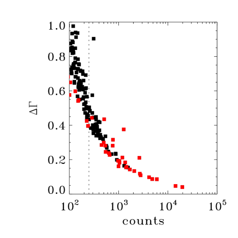
Figure 2: Plot of the uncertainty of $\Gamma$ as a function of the number of source counts in the X-ray spectrum. We cut the sample to sources with greater than 250 counts in order to include sources for which $\Delta\Gamma<0.5$. Red data points show where the data come from the E-CDF-S , while black data points come from COSMOS. The points lying above the main relation are those where absorption has been included in the fit.

2.6 Determining $\lambda_{\rm Edd}$

The primary goal of this study is to investigate the relationship between $\Gamma$ and $\lambda_{\rm Edd}$, which requires a measurement of the bolometric luminosity. For 207 COSMOS sources, we take bolometric luminosities presented in L12, which are derived from spectral energy distribution (SED) fitting, from observed 160 ${\mu}$m to hard X-rays. Bolometric luminosities for type 1 AGN are calculated in the rest frame 1 ${\mu}$m to 200 keV. These data do not exist for our E-CDF-S sources however. For these sources we use a bolometric correction to the 2-10 keV X-ray luminosity ($\kappa_{2-10}$) to estimate $L_{\rm Bol}$. Lusso et al. (2010) showed that this can be done reliably using $\kappa_{2-10}$ derived from the X-ray to optical spectral index, $\alpha_{\rm OX}$. $\alpha_{\rm OX}$ is normally calculated using the monochromatic luminosities at 2500 Å and 2 keV, however, we utilise the 3000 Å luminosity we already have at hand from the line measurements, measured from the optical spectra, and the 2-10 keV luminosity measured in the X-ray spectra and calibrate a relationship between $\kappa_{\rm 2-10}$ and $L_{\rm{X}}$/$L_{3000}$, using sources with known $L_{\rm Bol}$ in COSMOS. We utilise 32 sources with $L_{3000}$ measured from FMOS and where $L_{\rm{X}}$ and $L_{\rm Bol}$ are available for this analysis. Figure 3 shows that $\kappa_{\rm 2-10}$ and $L_{\rm{X}}$/$L_{3000}$ are indeed tightly correlated. We perform a linear regression analysis on these data, finding that log${}_{10}\kappa_{2-10}=-0.70$log₁₀($L_{\rm{X}}$/$L_{3000}$)+0.84. We then calculate $L_{\rm Bol}$ for the E-CDF-S sources using this relationship. Figure 3 also shows the comparison between $L_{\rm Bol}$ calculated in this manner and $L_{\rm Bol}$ from L12 with good agreement between the two. For our sample of X-ray bright AGN to which we restrict our analysis with $\Gamma$, 44 have $L_{\rm Bol}$ from L12 and 31 have $L_{\rm Bol}$ calculated using $\kappa_{\rm 2-10}$.

Figure 3: Left - $\kappa_{2-10}$ vs. $L_{\rm{X}}$/$L_{3000}$ for 32 sources in COSMOS with $L_{\rm{X}}$, $L_{3000}$ and $L_{\rm Bol}$ measured with SED fitting from L12. The line plotted through the data shows the results of a linear regression analysis. Right - Comparison of $L_{\rm Bol}$ calculated from SED fitting in L12 to $L_{\rm Bol}$ calculated using $L_{\rm{X}}$ and $\kappa_{\rm 2-10}$ derived from the relationship between $\kappa_{\rm 2-10}$ and $L_{\rm{X}}$/$L_{3000}$. The line shows the one to one relationship.

2.7 Radio properties of the sample

As the subject of this study is to probe the X-ray emission from the corona, we must account for other sources of X-ray emission intrinsic to the AGN. Radio loud AGN constitute $\sim$10% of the AGN population, the fraction of which may vary with luminosity and redshift (e.g. Jiang et al., 2007) and are known to exhibit X-ray emission attributable to synchrotron or synchro-Compton emission from a jet (Zamorani et al., 1981). As such we must exclude radio loud AGN from our study. We compile radio data on our sample, specifically to exclude radio loud sources from our analysis, but also to investigate the radio properties. Deep ($\sim 10\mu$Jy rms) VLA 1.4 GHz observations of both COSMOS and the E-CDF-S exist (Schinnerer et al., 2007; Miller et al., 2013). In COSMOS, we match the XMM-Newton sources to the radio sources, and in E-CDF-S, we take the matches from Bonzini et al. (2012). For 21 sources with a radio detection, we calculate the radio loudness parameter (Kellermann et al., 1989), R, which is defined as $f_{\rm 5GHz}/f_{4400}$. We extrapolate the observed 1.4 GHz flux density to rest-frame 5 GHz using a power-law slope of -0.8. For the 4400Å flux density, we extrapolate the observed R band flux density to rest-frame 4400Å using a power-law slope of -0.5. R band magnitudes were taken from Brusa et al. (2010) and Lehmer et al. (2005) for COSMOS and E-CDF-S respectively. For radio undetected sources, we calculate an upper limit on R assuming a $10\mu$Jy sensitivity in both fields. Figure 4 shows the distribution of R in the sample. We find six radio loud (R$>$100) sources in our sample, which we exclude from our analysis with $\Gamma$, leaving us with a sample of 69 radio quiet AGN. Using upper limits, we can rule out radio loudness in the undetected sources.

Figure 4: Distribution of radio loudness parameter, R, for sources with radio detections (empty histograms), where the solid histogram is for E-CDF-S sources. The hatched histogram shows upper limits on the sources with no radio detection, assuming $10\mu$Jy sensitivity.

3 What influences the physical conditions of the corona?

It is understood that the characteristic shape of the X-ray spectrum produced in the corona, parametrised by $\Gamma$, depends on the electron temperature, T_e, and the optical depth to electron scattering, $\tau_{es}$, but it is unknown how these conditions arise, and how they relate to the accretion flow. We explore the dependence of $\Gamma$ on the various accretion parameters in an attempt to understand what brings about the physical conditions of the corona. The parameters we explore in this work are $L_{\rm UV}$, $L_{\rm{X}}$, FWHM, $M_{\rm BH}$ and $\lambda_{\rm Edd}$.

3.1 $L_{\rm{X}}$ and redshift

In order to investigate the relationships between $\Gamma$ and FWHM, $M_{\rm BH}$ and $\lambda_{\rm Edd}$, we first check for any dependencies on $L_{\rm{X}}$ and redshift in our sample in order to rule out degeneracies, as correlations with $L_{\rm{X}}$ and redshift have been reported previously (Dai et al., 2004; Saez et al., 2008). Figure 5 plots these relationships. A Spearman rank correlation analysis shows that there are no significant correlations present between $\Gamma$ and $L_{\rm{X}}$  or $\Gamma$ and redshift within this sample. We do note however that at the lowest X-ray luminosities ($L_{\rm{X}}$$<3\times 10^{43}$ erg s^-1) that $\Gamma$ is systematically lower than at higher luminosities. While these are only 7 sources, we consider what affect if any they have on our results in a later section.

Figure 5: Plot of $\Gamma$ vs $L_{\rm{X}}$ and redshift, where top panels show individual measurements and bottom panels show binned averages. Spearman rank correlation coefficients and p-values are displayed, showing there are no significant correlations with either $L_{\rm{X}}$ or redshift, however, the lowest luminosity bin shows systematically lower $\Gamma$ values than the higher luminosity bins.

3.2 $L_{\rm UV}$, FWHM, $M_{\rm BH}$ and $\lambda_{\rm Edd}$

We next investigate the dependence on the observed quantities, the 3000 Å UV luminosity and FWHM of the lines and those derived quantities, black hole mass and $\lambda_{\rm Edd}$. The UV luminosity traces the accretion disc luminosity, and is thus related to the mass accretion rate, $\dot{m}$ ($L_{\rm acc}=\eta\dot{m}c^{2}$), whereas FWHM traces the gravitational potential. Furthermore, $L_{3000}$ and FWHM are the ingredients in the black hole mass calculation, which in turn is used in the determination of $\lambda_{\rm Edd}$. In Fig. 6, we show how $\Gamma$ depends on these four quantities.

Here we are using a combined sample of Mg ii and H$\alpha$ measurements for FWHM, $M_{\rm BH}$ and $\lambda_{\rm Edd}$. In the figure we distinguish between the two line measurements with different colouring. When considering the combined sample, if a source has a measurement from both lines, we use the H$\alpha$ measurement over the Mg ii measurement. For $\lambda_{\rm Edd}$, we also differentiate between cases where $L_{\rm Bol}$ has been determined using SED fitting (filled squares), or where it has been determined from $L_{\rm{X}}$/$L_{3000}$ (open squares).

A strong correlation with $L_{3000}$ is seen, which breaks at low luminosities ($L_{3000}\sim 10^{44}$ erg s^-1) and a strong anti-correlation with FWHM can be seen. These then cancel out here to give no dependence of $\Gamma$ on $M_{\rm BH}$. A strong correlation is then seen with $\lambda_{\rm Edd}$. The Spearman rank correlation test shows that there is a significant correlation between $\Gamma$ and $L_{3000}$ ($r_{\rm S}=0.57$ and $p=1.81\times 10^{-4}$, where $r_{\rm S}$ is the Spearman rank correlation coefficient and p is the probability of obtaining the absolute value of $r_{\rm S}$ at least as high as observed, under the assumption of the null hypothesis of zero correlation.), a significant anti-correlation ($p=$2.71$\times 10^{-4}$) between $\Gamma$ and the FWHM ($r_{\rm S}=$ -0.41) and a highly significant correlation ($p=$6.59$\times 10^{-8}$) between $\Gamma$ and $\lambda_{\rm Edd}$ ($r_{\rm S}=$0.60).

Despite the several ingredients used to derive $\lambda_{\rm Edd}$, this is by far the strongest correlation seen, stronger than with the observed quantities $L_{3000}$ and FWHM. This further confirms $\lambda_{\rm Edd}$ as the primary parameter influencing the physical conditions of the corona responsible for the shape of the X-ray spectrum, being the electron temperature and electron scattering optical depth. Furthermore, as the relationship with $L_{3000}$, which is linked to the mass accretion rate, shows a break at low luminosities, which is not evident in the relationship with $\lambda_{\rm Edd}$, which is related to the mass accretion rate scaled by the black hole mass, this implies that the Eddington rate is more important than mass accretion rate.

Also shown on these plots are the $\Gamma-$$\lambda_{\rm Edd}$ correlations previously reported by S08 and R09. Our results are consistent with S08 in the two highest bins of $\lambda_{\rm Edd}$, however our results diverge at lower values of $\lambda_{\rm Edd}$, with a flatter $\Gamma-$$\lambda_{\rm Edd}$ relationship. Our results are systematically higher than those reported in R09. We explore these differences further in section 4.2.2.

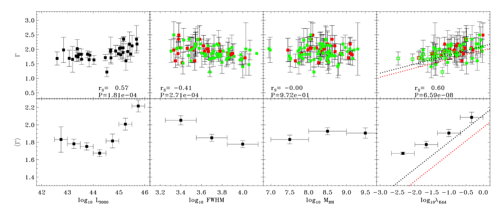
Figure 6: Plots of $\Gamma$ versus UV luminosity ($\lambda$=3000Å), FWHM (km s^-1), black hole mass ($M_{\odot}$) and $\lambda_{\rm Edd}$. Top panels show individual measurements, where red data points are measurements from the H$\alpha$ line, and green from the Mg ii line. For $\lambda_{\rm Edd}$, filed squares are data derived using $L_{\rm Bol}$ from SED fitting, whereas empty squares are data derived using $L_{\rm Bol}$ from $L_{\rm{X}}$/$L_{3000}$. Bottom panels show binned averages. The Spearman-rank correlation coefficient, $r_{\rm S}$, and the p-value are shown for each relationship. The black and red dotted lines are previous correlations reported on $\Gamma$-$\lambda_{\rm Edd}$ from S08 and R09 respectively.

For the two relationships between $\Gamma$ and FWHM and $\Gamma$ and $\lambda_{\rm Edd}$ where emission line measurements were used, we further the investigation in different subsamples: in two different redshift bins ($0.5<z<1.2$ and $1.2<z<2.1$), effectively splitting the sample in half, and considering measurements made by H$\alpha$ and Mg ii separately. Table 1 presents the results of Spearman rank and linear regression analysis of the $\Gamma$ vs. FWHM relationship for these different subsamples. The correlation is most significant in the full redshift range when using only the Mg ii measurements ($p=$1.32$\times 10^{-4}$), however the correlation is not significant ($p>0.1$) when considering only H$\alpha$ measurements, though this may be due to small number statistics. For the whole sample, we find that

$$\Gamma=(0.32\pm 0.05){\rm log}_{10}\lambda_{\rm Edd}+(2.27\pm 0.06)$$ (2)

Taking the two line measurements separately gives $\Gamma=(-0.49\pm 0.14)$log₁₀(FWHM/km s^-1)$+(3.72\pm 0.53)$ from H$\alpha$ and $\Gamma=(-1.02\pm 0.15)$log₁₀(FWHM/km s^-1)$+(5.70\pm 0.54)$ from Mg ii. The slopes are significantly different, at $>$3-$\sigma$. Fig. 7 shows the sample in the two redshift bins and for the two line measurements separately, along with the best fit lines.

Table 1: Table of Spearman rank correlation and linear regression analysis for $\Gamma$ vs.log₁₀FWHM for sources with a measurement from Mg ii or H$\alpha$ and with greater than 250 source counts in the X-ray spectrum. In the combined sample of Mg ii and H$\alpha$ measurements, if both exist for one source, the H$\alpha$ measurement is used over the Mg ii measurement. Column (1) is the redshift range used; (2) is the emission lines used for the FWHM; (3) is the total number of sources within each subsample; (4) is the Spearman rank coefficient; (5) is the null hypothesis probability; (6) is the gradient coefficient in the linear regression analysis, where $\Gamma=$m log₁₀FWHM+c; and (7) is the constant in this relationship.

redshift range	lines used	number in subsample	$R_{\rm S}$	$p$	m	c
(1)	(2)	(3)	(4)	(5)	(6)	(7)
0.5- 2.1	H$\alpha$ & MgII	73	-0.41	2.71$\times 10^{-4}$	-0.69$\pm$ 0.11	4.44$\pm$ 0.42
	H$\alpha$	25	-0.24	2.54$\times 10^{-1}$	-0.49$\pm$ 0.14	3.72$\pm$ 0.53
	MgII	65	-0.46	1.32$\times 10^{-4}$	-1.02$\pm$ 0.15	5.70$\pm$ 0.54
0.5- 1.2	H$\alpha$ & MgII	34	-0.49	3.53$\times 10^{-3}$	-0.86$\pm$ 0.14	5.13$\pm$ 0.52
	H$\alpha$	12	-0.25	4.30$\times 10^{-1}$	-0.71$\pm$ 0.17	4.58$\pm$ 0.64
	MgII	29	-0.63	2.88$\times 10^{-4}$	-1.23$\pm$ 0.18	6.48$\pm$ 0.68
1.2- 2.1	H$\alpha$ & MgII	39	-0.36	2.52$\times 10^{-2}$	-0.43$\pm$ 0.19	3.40$\pm$ 0.71
	H$\alpha$	13	-0.20	5.17$\times 10^{-1}$	-0.01$\pm$ 0.33	1.97$\pm$ 1.17
	MgII	36	-0.35	3.68$\times 10^{-2}$	-0.61$\pm$ 0.24	4.09$\pm$ 0.91

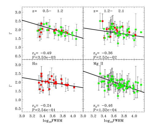
Figure 7: Plots of $\Gamma$ vs the FWHM of the emission lines in four subsamples: two redshift bins, $0.5<z<1.2$ and $1.2<z<2.1$ (top panels) and for the measurements from H$\alpha$ and Mg ii separately (bottom panels).

We also carry out Spearman rank correlation analysis and linear regression analysis on the $\Gamma$ vs. $\lambda_{\rm Edd}$ relationship for the different subsamples. The results are presented in Table 2. The correlation is most significant in the full redshift range when using the two line measurements together ($p=$6.59$\times 10^{-8}$). The correlation is significant ($p<0.1$) in all redshift bins, however, not for measurements made with H$\alpha$ in the highest redshift bin. This is again likely due to small number statistics. For the whole sample we find that

$$\Gamma=(-0.69\pm 0.11){\rm log}_{10}{\rm(FWHM/kms}^{-1})+(4.44\pm 0.42)$$ (3)

The slope of the correlations for H$\alpha$ and Mg ii agree very well with each other with $\Gamma=(0.34\pm 0.07)$log₁₀$\lambda_{\rm Edd}$$+(2.34\pm 0.09)$ for H$\alpha$ and $\Gamma=(0.35\pm 0.05)$log₁₀$\lambda_{\rm Edd}$$+(2.28\pm 0.06)$ for Mg ii and for all redshift bins. This supports the claim by Matsuoka et al. (2013) that the two line measurements give consistent black hole mass estimates. We plot $\Gamma$ versus $\lambda_{\rm Edd}$ in the two redshift bins and for the two lines separately in Figure 8, along with the best fit lines.

Table 2: Table of Spearman rank correlation and linear regression analysis for $\Gamma$ vs. log₁₀$\lambda_{\rm Edd}$, for sources with $M_{\rm BH}$ from Mg ii or H$\alpha$, an estimate of the bolometric luminosity and those with greater than 250 source counts in the X-ray spectrum. In the combined sample of Mg ii and H$\alpha$ measurements, if both exist for one source, the H$\alpha$ measurement is used over the Mg ii measurement. Column (1) is the redshift range used; (2) is the emission lines used for the estimation of the black hole mass; (3) is the total number of sources within each subsample; (4) is the Spearman rank coefficient; (5) is the null hypothesis probability; (6) is the gradient coefficient in the linear regression analysis, where $\Gamma$=m log₁₀$\lambda_{\rm Edd}$+c; and (7) is the constant in this relationship.

redshift range	lines used	number in subsample	$R_{\rm S}$	$p$	m	c
(1)	(2)	(3)	(4)	(5)	(6)	(7)
0.5- 2.1	H$\alpha$ & MgII	69	0.60	6.59$\times 10^{-8}$	0.32$\pm$ 0.05	2.27$\pm$ 0.06
	H$\alpha$	22	0.60	2.94$\times 10^{-3}$	0.34$\pm$ 0.07	2.34$\pm$ 0.09
	MgII	64	0.58	6.63$\times 10^{-7}$	0.35$\pm$ 0.05	2.28$\pm$ 0.06
0.5- 1.2	H$\alpha$ & MgII	33	0.74	8.82$\times 10^{-7}$	0.39$\pm$ 0.06	2.39$\pm$ 0.07
	H$\alpha$	11	0.67	2.33$\times 10^{-2}$	0.43$\pm$ 0.09	2.46$\pm$ 0.11
	MgII	29	0.75	2.82$\times 10^{-6}$	0.43$\pm$ 0.07	2.39$\pm$ 0.07
1.2- 2.1	H$\alpha$ & MgII	36	0.53	8.38$\times 10^{-4}$	0.27$\pm$ 0.08	2.10$\pm$ 0.09
	H$\alpha$	11	0.50	1.17$\times 10^{-1}$	0.23$\pm$ 0.15	2.18$\pm$ 0.14
	MgII	35	0.52	1.22$\times 10^{-3}$	0.27$\pm$ 0.08	2.08$\pm$ 0.09

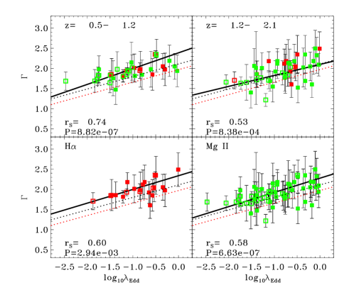
Figure 8: Plots of $\Gamma$ vs $\lambda_{\rm Edd}$ for four subsamples: two redshift bins, $0.5<z<1.2$ and $1.2<z<2.1$ (top panels) where red data points are measurements from the H$\alpha$ line, and green from the Mg ii line. Filled symbols are data derived using $L_{\rm Bol}$ from SED fitting, whereas empty symbols are data derived using $L_{\rm Bol}$ from $L_{\rm{X}}$/$L_{3000}$. The bottom panels show the measurements from H$\alpha$ and Mg ii separately in the full redshift range. The black and red dotted lines are previous correlations reported on $\Gamma$-$\lambda_{\rm Edd}$ from S08 and R09.

3.3 Radio loud sources

In section 2.7, we investigated the radio properties of the sample, finding six sources which are radio loud (R$>$100). We excluded these sources from our sample as radio loud AGN have significant X-ray emission from their jets, and thus contaminate the coronal emission which interests us. However, we briefly explore the properties of the radio loud sources here. Fig 9 plots the $\Gamma$-$\lambda_{\rm Edd}$ relationship found in the previous section, here with only sources with radio detections. We colour code the data points by radio loudness. We find that radio loud sources are generally consistent with this trend, with the exception of two sources with high Eddington ratios ($\lambda_{\rm Edd}$$>0.3$).

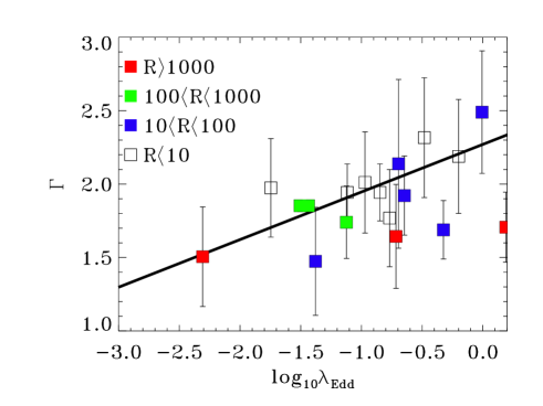
Figure 9: $\Gamma$ vs. $\lambda_{\rm Edd}$ for sources with radio detections only, where colour corresponds to radio loudness, parametrised by R. The solid line is the best fit line to the full sample found in the previous section, when excluding radio loud sources. We find that radio loud sources are generally consistent with this trend, with the exception of sources with high Eddington ratios ($\lambda_{\rm Edd}$$>0.3$).

4 discussion

4.1 Accounting for degeneracies and biases

4.1.1 Low $L_{\rm{X}}$ sources

We noted in section 3.1 that at low X-ray luminosities ($L_{\rm{X}}$$<3\times 10^{43}$  erg s^-1), $\Gamma$ is systematically lower. While there are only 7 sources at these low luminosities, and a Spearman rank correlation test tells us there is a lack of a significant correlation between $\Gamma$ and $L_{\rm{X}}$ in our sample, we check the effects on our results when excluding these sources at low $L_{\rm{X}}$. When doing this, we find that a significant correlation between $\Gamma$ and $\lambda_{\rm Edd}$ persists, with $p=7.7\times 10^{-6}$. Linear regression analysis of this subsample gives $\Gamma=(0.35\pm 0.05)$log₁₀$\lambda_{\rm Edd}$$+(2.30\pm 0.06)$. We plot these data with the best fit trend line in Fig. 10.

4.1.2 The soft X-ray excess and FWHM degeneracy

When it was reported by Boller et al. (1996) and Laor et al. (1997) that the soft X-ray (0.2-2 keV) power-law index correlated well with the FWHM of the H$\beta$ line, also interpreted as a dependence on accretion rate, it was thought that this may have been related to the soft X-ray excess seen in unobscured AGN (e.g. Arnaud et al., 1985; Turner & Pounds, 1989). This feature is strong in narrow line Seyfert 1s (Boller et al., 1996), which have low FWHMs (Osterbrock & Pogge, 1985), and as such a strong soft excess could cause a steepening of the X-ray spectrum leading to higher values of $\Gamma$ for low FWHM sources. Brandt et al. (1997) later reported a correlation between $\Gamma$ in the 2-10 keV band and the FWHM of the H$\beta$ line, where this band is less affected by the soft excess, leading to the conclusion that both the soft excess and the power-law are affected by the accretion rate. We attempt to further rule out the effect of the soft excess on the power-law by considering the 4-10 keV rest-frame band where the X-ray spectrum should be completely independent of the soft excess. We rerun our analysis described in section 2.5 with this restriction, however, in doing this we decrease the number of spectral counts. We therefore lower the count cut that we make using the 2-10 keV spectrum of 250 counts to 100 counts in the 4-10 keV band. Despite this we still find a significant correlation between $\Gamma$ and $\lambda_{\rm Edd}$ with a p-value of 0.002. This confirms that the soft excess does not substantially contribute to the $\Gamma$-$\lambda_{\rm Edd}$ relationship.

We next consider the relationship between FWHM and $\lambda_{\rm Edd}$ (Boroson & Green, 1992), and the degeneracy it may introduce in our work. As our aim here is to rule out degeneracies where possible, we investigate the effect of making a cut in FWHM. We note that the correlation of $\Gamma$ vs. FWHM appears to be driven by sources with FWHM$<4000$ km s^-1, and thus we investigate the $\Gamma$-$\lambda_{\rm Edd}$ relationship for sources with FWHM$>4000$ km s^-1 in our sample. In doing so, however, we still find a significant correlation between $\Gamma$ and $\lambda_{\rm Edd}$ with a p-value of 0.005, which effectively rules out a bias from low FWHM sources, and rules out degeneracy with FWHM. A linear regression analysis finds that $\Gamma=(0.12\pm 0.07)$log₁₀$\lambda_{\rm Edd}$$+(1.98\pm 0.10)$. We plot the subsample with the best fit trend line in Fig. 10.

4.1.3 Contribution from reflection

It is important to consider what effects reflection of X-rays, from either the accretion disc or the circumnuclear torus may have on our results. In our X-ray spectral fitting we use a simple power-law to characterise the spectrum, however in reality reflection features are present. As the geometry of the torus is expected to change with X-ray luminosity and redshift (e.g. Lawrence, 1991; Ueda et al., 2003; Hasinger, 2008; Brightman & Ueda, 2012), this component should not be neglected. In order to account for this, we utilise the X-ray spectral torus models of Brightman & Nandra (2011), which describe the X-ray spectra of AGN surrounded by a torus of spherical geometry. In order to explain the decrease in the AGN obscured fraction with increasing X-ray luminosity, and the increase with redshift, new work from Ueda, et al (in preparation) have calculated the dependence of the torus opening angle on these parameters. Essentially the torus opening angle increases with increasing X-ray luminosity and decreases with increasing redshift. The effect of this on the observed $\Gamma$ is for $\Gamma$ to decrease towards smaller opening angles, and hence greater covering factors, due to greater reflection from the torus which has a flat spectrum. We use this prescription when fitting our spectra with this torus model, where the viewing angle is set such that the source is unobscured, the $N_{\rm{H}}$ through the torus is set to $10^{24}$ cm^-2 and the opening angle depends on the X-ray luminosity and redshift. We follow the same spectral fitting technique as described in section 2.5, and study the results. We find that the correlation between $\Gamma$ and $\lambda_{\rm Edd}$ remains highly significant with a p-value of $2.5\times 10^{-5}$. We note that the observed $\Gamma$ produced by this torus model changes by a maximum of 0.06 in the 2-10 keV range for the extremes of the parameter space, while we observe changes of greater than 0.2. It is therefore unlikely that reflection affects our results. S08 also investigated the effects of reflection in their analysis, finding only two sources where a reflection component was significantly detected. This low detection rate is expected due to the high luminosity nature of the sources at high redshifts.

4.1.4 X-ray variability

We briefly check if X-ray variability has an effect on our results, specifically if the outliers in our relationships may be explained by this. Lanzuisi, et al (in preparation) have conducted an investigation into AGN variability for XMM-COSMOS sources. They find that 6 of the sources in our sample are variable in X-rays through the detection of excess variance. We find however, that these sources lie consistently on the best fit relations found here, leading us to the conclusion that variability is not likely to affect our results. Papadakis et al. (2009) directly investigated the relationship between $\Gamma$ and AGN variability, finding that $\Gamma$ correlates with the characteristic frequency in the power spectrum when normalised by the black hole mass. They then used the result of McHardy et al. (2006), which showed that this normalised characteristic frequency is correlated to the accretion rate, to also show in an independent manner to what we have shown here, that $\Gamma$ is correlated with accretion rate. Their result held true even when using the mean spectral slope of their data. This result is relevant here, as we have used time averaged spectra, which Papadakis et al. (2009) have shown produces consistent results to time resolved spectroscopy.

4.1.5 Chandra/XMM-Newton cross-calibration

We use both Chandra and XMM-Newton data in our analysis, with XMM-Newton data in COSMOS and Chandra data in the E-CDF-S . However, it has been found that a systematic difference between measurements made by the two observatories of the same source exists (L13). Most relevant to our work is a systematic difference of up to 20% in $\Gamma$, which may seriously bias our results. We investigate this issue by performing our analysis using the Chandra data available in COSMOS. We extract the Chandra spectra as described in section 2.3 for the E-CDF-S sources and analyse the data in the same way. While the sample size is reduced to 44 sources with $\Gamma$ and $\lambda_{\rm Edd}$ due to the smaller coverage of the Chandra observations in COSMOS and the lower number of source counts per spectrum, our main result is maintained. For $\Gamma$ vs. $\lambda_{\rm Edd}$, the Spearman rank correlation analysis reveals a significant correlation with $p=2.42\times 10^{-3}$ and linear regression analysis finds that $\Gamma=(0.32\pm 0.05)$log₁₀$\lambda_{\rm Edd}$$+(2.27\pm 0.06)$, which is in very good agreement with the joint Chandra/XMM-Newton analysis. These data are plotted with the best fitting trend line in Fig. 10.

Figure 10: Plots of $\Gamma$ vs $\lambda_{\rm Edd}$ when excluding sources with FWHM$<$4000 km s^-1 (top) and sources with $L_{\rm{X}}$$<10^{43.5}$  erg s^-1 (middle) in order to break any degeneracy with these parameters. The lowest panel shows $\Gamma$ vs $\lambda_{\rm Edd}$ when using Chandra data in COSMOS instead of XMM-Newton data in order to investigate the effect of the cross-normalisation between these telescopes.

4.2 Comparison with previous studies

4.2.1 X-ray spectral analysis in COSMOS

Recent work by L13 has presented a spectral analysis of bright Chandra-COSMOS sources, the aim of which was to determine the intrinsic absorption in the spectrum, as well as $\Gamma$. Their work also presents analysis of XMM-Newton spectra of the Chandra counterparts. Their analysis differs from our own as they utilise the fuller 0.5-7 keV band pass and sources with greater than 70 net counts, whereas we limit ourselves to analysis in the rest-frame 2-10 keV band and spectra with at least 250 counts. We investigate the differences in these methods by comparing the results for 129 common sources, in particular with respect to absorption. As we restrict ourselves to rest-frame energies greater than 2 keV, we are not sensitive to $N_{\rm{H}}$$\lesssim 10^{22}$ cm^-2, whereas L13 utilise a fuller band pass and as such are thus sensitive to lower levels of absorption. While we only detect absorption in one source from our COSMOS sample, this is not a common source with L13. From the common sources, they detect absorption in six sources (XMM-IDs 28, 30, 34, 38, 66 and 71), however the measured $N_{\rm{H}}$ is $<5\times 10^{21}$ cm^-2 in all of these, and thus will have no affect on our measurement of $\Gamma$. When comparing $\Gamma$ measurements between the two analyses, there is good agreement, with the difference being within our measurement error and there being no systematic offsets.

4.2.2 $\Gamma$-$\lambda_{\rm Edd}$ correlation

In Figs. 6 & 8, we have compared our results on the $\Gamma$-$\lambda_{\rm Edd}$ correlation with two previous works by S08 and R09. We found that for the whole sample, our binned averages were consistent with the results of S08 in the highest $\lambda_{\rm Edd}$ bins, while overall systematically higher than those of R09. At lower $\lambda_{\rm Edd}$ values our $\Gamma$ measurements lie above these previous correlations.

The results from S08 were based on a sample of 35 moderate- to high-luminosity radio quiet AGN having high quality optical and X-ray spectra, based on individual observations, and including nearby sources and those up to z=3.2. The black hole masses were estimated from the H$\beta$ line. The results of R09 are based on 403 sources from the SDSS/XMM-Newton quasar survey of Young et al. (2009), which span a wide range in X-ray luminosity ($10^{43}<$$L_{\rm{X}}$$<10^{45.5}$  erg s^-1) and redshift (0.1$<z<4.5$), with black hole masses based on H$\beta$, Mg ii and C iv. The work presented here is based on a sample of 69 sources with black hole estimates based on H$\alpha$ and Mg ii, and samples X-ray luminosities in the range of $10^{42.5}<$$L_{\rm{X}}$$<10^{45.5}$  erg s^-1 and the redshift range of $0.5<z<2.1$.

Our analysis finds that $\Gamma=(0.32\pm 0.05)$log₁₀$\lambda_{\rm Edd}$$+(2.27\pm 0.06)$. Meanwhile, S08 find that $\Gamma=(0.31\pm 0.01)$log₁₀$\lambda_{\rm Edd}$$+(2.11\pm 0.01)$ and R09 find that $\Gamma=(0.31\pm 0.06)$log₁₀$\lambda_{\rm Edd}$$+(1.97\pm 0.02)$. The slope of our $\Gamma$-$\lambda_{\rm Edd}$ correlation is in excellent agreement with these two previous works. The constant in the relationship is higher than both studies by 3-$\sigma$. This may be due to differing methods of X-ray spectral fitting. Here we use Cash statistics in our analysis, whereas previous works have used $\chi^{2}$, the two being known to produce systematic differences in $\Gamma$ (Tozzi et al., 2006).

Furthermore, R09 reported significantly differing slopes for $\Gamma-$$\lambda_{\rm Edd}$(H$\beta$) and $\Gamma-$$\lambda_{\rm Edd}$(Mg ii), where the H$\beta$ slope was steeper. We also compared our slopes for H$\alpha$ and Mg ii, but found no such difference. We make a comparison to the results from S08 and R09 considering the different lines separately in Table 3. For the Mg ii line, only R09 have presented results and we find that our results are consistent with these within 2-$\sigma$. We present here for the first time results based on H$\alpha$ alone, however, our H$\alpha$ results are in very good agreement with the H$\beta$ results in S08, though the difference between these results and the H$\beta$ results in R09 is 3-$\sigma$.

The differing results between H$\beta$ and Mg ii reported in R09 were attributed to uncertainties in the measurement of Mg ii. However, Matsuoka et al. (2013), which describes the measurements of H$\alpha$ and Mg ii used in this sample find very good agreements between these lines, which subsequently has lead to the good agreement we find between them here.

Table 3: A summary of the results of the best fit line to the $\Gamma$-$\lambda_{\rm Edd}$ correlation from this work and those of S08 and R09, for line measurements made from H$\alpha$, H$\beta$ and Mg ii. Column (1) is the sample used, column (2) is the lines used, column (3) is the slope of the relationship and column (4) is the intercept

Sample	Lines	m	c
(1)	(2)	(3)	(4)
This work	H$\alpha$ & Mg ii	$0.32\pm 0.05$	$2.27\pm 0.06$
R09	H$\beta$, Mg ii & C iv	$0.31\pm 0.06$	$1.97\pm 0.02$
This work	Mg ii	$0.35\pm 0.05$	$2.28\pm 0.06$
R09	Mg ii	$0.24\pm 0.05$	$1.98\pm 0.02$
This work	H$\alpha$	$0.34\pm 0.07$	$2.28\pm 0.06$
S08	H$\beta$	$0.31\pm 0.01$	$2.11\pm 0.01$
R09	H$\beta$	$0.58\pm 0.11$	$1.99\pm 0.04$

4.3 Wider implications of our results

We have confirmed previous results that $\lambda_{\rm Edd}$, rather than $L_{\rm UV}$, $L_{\rm{X}}$, FWHM or $M_{\rm BH}$, is the parameter which most strongly correlates with the X-ray spectral index, $\Gamma$, and hence is responsible for driving the physical conditions of the corona responsible for the shape of the X-ray spectrum, being the electron temperature and electron scattering optical depth. This result enables models of accretion physics in AGN to be constrained. As this correlation is stronger than the $\Gamma$-$L_{3000}$ correlation, where $L_{3000}$ is related to the mass accretion rate, $\dot{m}$ and $\lambda_{\rm Edd}$ is related to the mass accretion rate scaled by $M_{\rm BH}$, then the coronal conditions must depend on both mass accretion rate and black hole mass, despite there being no correlation with black hole mass itself. A possible interpretation of the correlation between $\Gamma$ and $\lambda_{\rm Edd}$ is that as $\lambda_{\rm Edd}$ increases, the accretion disc becomes hotter, with enhanced emission. This enhanced emission cools the electron corona more effectively, leading to a lower election temperature, electron scattering optical depth, or both. $\Gamma$ thus increases as these quantities decrease.

As pointed out by previous authors on this subject, a statistically significant relationship between $\Gamma$ and $\lambda_{\rm Edd}$ allows for an independent estimate of $\lambda_{\rm Edd}$ for AGN from their X-ray spectra alone. While the dispersion in this relationship means that this is not viable for single sources, it could be used on large samples, for example those produced by eROSITA. eROSITA is due for launch in 2014 and will detect up to 3 million AGN with X-ray spectral coverage up to 10 keV. These results could be valuable in placing estimates on the accretion history of the universe using these new data.

5 Conclusions

We have presented an X-ray spectral analysis of broad-lined radio-quiet AGN in the extended Chandra Deep Field South and COSMOS surveys with black hole mass estimates. The results are as follows:

• We confirm a statistically significant correlation between the rest-frame 2-10 keV photon index, $\Gamma$, and the FWHM of the optical broad emission lines, found previously by Brandt et al. (1997). A linear regression analysis reveals that $\Gamma=(-0.69\pm 0.11)$log₁₀(FWHM/km s^-1)$+(4.44\pm 0.42)$.

• A statistically signifiant correlation between $\Gamma$ and $\lambda_{\rm Edd}$ is also confirmed, as previously reported in S06, S08 and R09. The relationship between $\Gamma$ and $\lambda_{\rm Edd}$ is highly significant with a chance probability of 6.59$\times 10^{-8}$. A linear regression analysis reveals that $\Gamma=(0.32\pm 0.05)$log₁₀$\lambda_{\rm Edd}$$+(2.27\pm 0.06)$, in very good agreement with S08 and R09. The correlation with $\lambda_{\rm Edd}$ is the strongest of all parameters tested against $\Gamma$, indicating that it is the Eddington rate, which is related to the mass accretion rate scaled by the black hole mass, that drives the physical conditions of the corona responsible for the X-ray emission. We find no statistically significant relationship between $\Gamma$ and black hole mass by itself.

• We present this analysis for the first time at high redshift with the H$\alpha$ line, finding that the $\Gamma$-$\lambda_{\rm Edd}$ correlation agrees very well for measurements with H$\alpha$ and with Mg ii. The Mg ii correlation is consistent with the results of R09 within 3-$\sigma$ and the H$\alpha$ correlation is consistent with the H$\beta$ results from S08.

References

- Arnaud et al. (1985) Arnaud K. A., Branduardi-Raymont G., Culhane J. L., Fabian A. C., Hazard C., McGlynn T. A., Shafer R. A., Tennant A. F., Ward M. J., 1985, MNRAS, 217, 105
- Boller et al. (1996) Boller T., Brandt W. N., Fink H., 1996, AA, 305, 53
- Bonzini et al. (2012) Bonzini M., Mainieri V., Padovani P., Kellermann K. I., Miller N., Rosati P., Tozzi P., Vattakunnel S., Balestra I., Brandt W. N., Luo B., Xue Y. Q., 2012, ApJS, 203, 15
- Boroson & Green (1992) Boroson T. A., Green R. F., 1992, ApJS, 80, 109
- Brandt et al. (1997) Brandt W. N., Mathur S., Elvis M., 1997, MNRAS, 285, L25
- Brightman & Nandra (2011) Brightman M., Nandra K., 2011, MNRAS, 413, 1206
- Brightman & Ueda (2012) Brightman M., Ueda Y., 2012, MNRAS, 423, 702
- Broos et al. (2010) Broos P. S., Townsley L. K., Feigelson E. D., Getman K. V., Bauer F. E., Garmire G. P., 2010, ApJ, 714, 1582
- Brusa et al. (2010) Brusa M., Civano F., Comastri A., Miyaji T., Salvato M., Zamorani G., Cappelluti N., Fiore F., 2010, ApJ, 716, 348
- Cappelluti et al. (2009) Cappelluti N., Brusa M., Hasinger G., Comastri A., Zamorani G., Finoguenov A., Gilli R., Puccetti S., Miyaji T., Salvato M., Vignali C., Aldcroft T., Böhringer H., Brunner H., Civano F., Elvis M., Fiore F., 2009, AA, 497, 635
- Cash (1979) Cash W., 1979, ApJ, 228, 939
- Civano et al. (2012) Civano F., Elvis M., Brusa M., Comastri A., Salvato M., Zamorani G., Aldcroft T., Bongiorno A., Capak P., Cappelluti N., Cisternas M., 2012, ApJS, 201, 30
- Dai et al. (2004) Dai X., Chartas G., Eracleous M., Garmire G. P., 2004, ApJ, 605, 45
- Elvis et al. (2009) Elvis M., Civano F., Vignali C., Puccetti S., Fiore F., Cappelluti N., Aldcroft T. L., Fruscione A., Zamorani G., Comastri A., Brusa M., Gilli R., Miyaji T., Damiani F., Koekemoer A. M., Finoguenov A., Brunner 2009, ApJS, 184, 158
- Fanali et al. (2013) Fanali R., Caccianiga A., Severgnini P., Della Ceca R., Marchese E., Carrera F. J., Corral A., Mateos S., 2013, ArXiv e-prints
- George et al. (2000) George I. M., Turner T. J., Yaqoob T., Netzer H., Laor A., Mushotzky R. F., Nandra K., Takahashi T., 2000, ApJ, 531, 52
- Giacconi et al. (2002) Giacconi R., Zirm A., Wang J., Rosati P., Nonino M., Tozzi P., Gilli R., Mainieri V., Hasinger G., Kewley L., Bergeron J., Borgani S., Gilmozzi R., Grogin N., Koekemoer A., Schreier E., Zheng W., Norman C., 2002, ApJS, 139, 369
- Greene & Ho (2005) Greene J. E., Ho L. C., 2005, ApJ, 630, 122
- Haardt & Maraschi (1991) Haardt F., Maraschi L., 1991, ApJL, 380, L51
- Haardt & Maraschi (1993) Haardt F., Maraschi L., 1993, ApJ, 413, 507
- Hasinger (2008) Hasinger G., 2008, AA, 490, 905
- Jiang et al. (2007) Jiang L., Fan X., Ivezić Ž., Richards G. T., Schneider D. P., Strauss M. A., Kelly B. C., 2007, ApJ, 656, 680
- Jin et al. (2012) Jin C., Ward M., Done C., 2012, MNRAS, 425, 907
- Kellermann et al. (1989) Kellermann K. I., Sramek R., Schmidt M., Shaffer D. B., Green R., 1989, AJ, 98, 1195
- Laird et al. (2009) Laird E. S., Nandra K., Georgakakis A., Aird J. A., Barmby P., Conselice C. J., Coil A. L., Davis M., Faber S. M., Fazio G. G., Guhathakurta P., Koo D. C., Sarajedini V., Willmer C. N. A., 2009, ApJS, 180, 102
- Lanzuisi et al. (2013) Lanzuisi G., Civano F., Elvis M., Salvato M., Hasinger G., Vignali C., Zamorani G., Aldcroft T., Brusa M., Comastri A., Fiore F., Fruscione A., Gilli R., Ho L. C., Mainieri V., Merloni A., Siemiginowska A., 2013, ArXiv e-prints
- Laor et al. (1997) Laor A., Fiore F., Elvis M., Wilkes B. J., McDowell J. C., 1997, ApJ, 477, 93
- Lawrence (1991) Lawrence A., 1991, MNRAS, 252, 586
- Lehmer et al. (2005) Lehmer B. D., Brandt W. N., Alexander D. M., Bauer F. E., Schneider D. P., Tozzi P., Bergeron J., Garmire G. P., Giacconi R., Gilli R., Hasinger G., Hornschemeier A. E., Koekemoer A. M., Mainieri V., Miyaji T., Nonino M., 2005, ApJS, 161, 21
- Lu & Yu (1999) Lu Y., Yu Q., 1999, ApJL, 526, L5
- Luo et al. (2008) Luo B., Bauer F. E., Brandt W. N., Alexander D. M., Lehmer B. D., Schneider D. P., Brusa M., Comastri A., Fabian A. C., Finoguenov A., Gilli R., Hasinger G., Hornschemeier A. E., Koekemoer A., Mainieri V., Paolillo M., Rosati P., 2008, ApJS, 179, 19
- Lusso et al. (2012) Lusso E., Comastri A., Simmons B. D., Mignoli M., Zamorani G., Vignali C., Brusa M., Shankar F., Lutz D., Trump J. R., Maiolino R., Gilli R., Bolzonella M., Puccetti S., Salvato M., Impey C. D., Civano F., Elvis M., Mainieri V., 2012, MNRAS, 425, 623
- Lusso et al. (2010) Lusso E., Comastri A., Vignali C., Zamorani G., Brusa M., Gilli R., Iwasawa K., Salvato M., Civano F., Elvis M., Merloni A., Bongiorno A., Trump J. R., Koekemoer A. M., Schinnerer E., Le Floc’h E., Cappelluti N., 2010, AA, 512, A34+
- Mainieri et al. (2007) Mainieri V., Hasinger G., Cappelluti N., Brusa M., Brunner H., Civano F., Comastri A., Elvis M., Finoguenov A., Fiore F., Gilli R., Lehmann I., Silverman J., Tasca L., Vignali C., Zamorani G., Schinnerer E., Impey C., 2007, ApJS, 172, 368
- Matsuoka et al. (2013) Matsuoka K., Silverman J. D., Schramm M., Steinhardt C. L., Nagao T., Kartaltepe J., Sanders D. B., Treister E., Hasinger G., 2013, ArXiv e-prints
- McHardy et al. (2006) McHardy I. M., Koerding E., Knigge C., Uttley P., Fender R. P., 2006, Nature, 444, 730
- McLure & Jarvis (2002) McLure R. J., Jarvis M. J., 2002, MNRAS, 337, 109
- Miller et al. (2013) Miller N. A., Bonzini M., Fomalont E. B., Kellermann K. I., Mainieri V., Padovani P., Rosati P., Tozzi P., Vattakunnel S., 2013, ApJS, 205, 13
- Mushotzky (1984) Mushotzky R. F., 1984, Advances in Space Research, 3, 157
- Nandra & Pounds (1994) Nandra K., Pounds K. A., 1994, MNRAS, 268, 405
- Osterbrock & Pogge (1985) Osterbrock D. E., Pogge R. W., 1985, ApJ, 297, 166
- Papadakis et al. (2009) Papadakis I. E., Sobolewska M., Arevalo P., Markowitz A., McHardy I. M., Miller L., Reeves J. N., Turner T. J., 2009, AA, 494, 905
- Ponti et al. (2012) Ponti G., Papadakis I., Bianchi S., Guainazzi M., Matt G., Uttley P., Bonilla N. F., 2012, AA, 542, A83
- Pounds et al. (1995) Pounds K. A., Done C., Osborne J. P., 1995, MNRAS, 277, L5
- Pounds et al. (1990) Pounds K. A., Nandra K., Stewart G. C., George I. M., Fabian A. C., 1990, Nature, 344, 132
- Rangel et al. (2013) Rangel C., Nandra K., Laird E. S., Orange P., 2013, MNRAS, 428, 3089
- Risaliti et al. (2009) Risaliti G., Young M., Elvis M., 2009, ApJL, 700, L6
- Rybicki & Lightman (1986) Rybicki G. B., Lightman A. P., 1986, Radiative Processes in Astrophysics. Radiative Processes in Astrophysics, by George B. Rybicki, Alan P. Lightman, pp. 400. ISBN 0-471-82759-2. Wiley-VCH , June 1986.
- Saez et al. (2008) Saez C., Chartas G., Brandt W. N., Lehmer B. D., Bauer F. E., Dai X., Garmire G. P., 2008, AJ, 135, 1505
- Schinnerer et al. (2007) Schinnerer E., Smolčić V., Carilli C. L., Bondi M., Ciliegi P., Jahnke K., Scoville N. Z., Aussel H., Bertoldi F., Blain A. W., Impey C. D., Koekemoer A. M., Le Fevre O., Urry C. M., 2007, ApJS, 172, 46
- Shakura & Sunyaev (1973) Shakura N. I., Sunyaev R. A., 1973, AA, 24, 337
- Shemmer et al. (2006) Shemmer O., Brandt W. N., Netzer H., Maiolino R., Kaspi S., 2006, ApJL, 646, L29
- Shemmer et al. (2008) Shemmer O., Brandt W. N., Netzer H., Maiolino R., Kaspi S., 2008, ApJ, 682, 81
- Sunyaev & Titarchuk (1980) Sunyaev R. A., Titarchuk L. G., 1980, AA, 86, 121
- Tananbaum et al. (1979) Tananbaum H., Avni Y., Branduardi G., Elvis M., Fabbiano G., Feigelson E., Giacconi R., Henry J. P., Pye J. P., Soltan A., Zamorani G., 1979, ApJL, 234, L9
- Tozzi et al. (2006) Tozzi P., Gilli R., Mainieri V., Norman C., Risaliti G., Rosati P., Bergeron J., Borgani S., Giacconi R., Hasinger G., Nonino M., Streblyanska A., Szokoly G., Wang J. X., Zheng W., 2006, A&A, 451, 457
- Turner & Pounds (1989) Turner T. J., Pounds K. A., 1989, MNRAS, 240, 833
- Ueda et al. (2003) Ueda Y., Akiyama M., Ohta K., Miyaji T., 2003, ApJ, 598, 886
- Vestergaard & Wilkes (2001) Vestergaard M., Wilkes B. J., 2001, ApJS, 134, 1
- Wang et al. (2004) Wang J.-M., Watarai K.-Y., Mineshige S., 2004, ApJL, 607, L107
- Xue et al. (2011) Xue Y. Q., Luo B., Brandt W. N., Bauer F. E., Lehmer B. D., Broos P. S., Schneider D. P., Alexander D. M., Brusa M., Comastri A., Fabian A. C., Gilli R., Hasinger G., Hornschemeier A. E., Koekemoer A., Liu T., Mainieri V., 2011, ApJS, 195, 10
- Young et al. (2009) Young M., Elvis M., Risaliti G., 2009, ApJS, 183, 17
- Zamorani et al. (1981) Zamorani G., Henry J. P., Maccacaro T., Tananbaum H., Soltan A., Avni Y., Liebert J., Stocke J., Strittmatter P. A., Weymann R. J., Smith M. G., Condon J. J., 1981, ApJ, 245, 357