SPIN AND PARITY IN THE $WH\rightarrow\ell\nu b\bar{b}$ CHANNEL AT THE D0 EXPERIMENT

We probe the spin ($J$) and parity ($P$) of the Standard Model Scalar (SMS) using existing searches sensitive to its production rate and kinematic properties. In particular, we search for the SMS decaying to a pair of $b$-quarks produced in association with a $W$ boson decaying leptonically. By exploiting the differences in kinematic observables, namely the transverse mass of the final state products ($M_{T}$), we attempt to distinguish between three possible $J^{P}$ hypotheses: the standard model prediction ($J^{P}=0^{+}$), a pseudoscalar ($J^{P}=0^{-}$), and a graviton-like particle ($J^{P}=2^{+}$). With $9.7$ fb^-1 of data collected at the D0 experiment we show the expected sensitivity to different spin and parity hypotheses.

1 Introduction

Following the discovery of a boson consistent with the predicted Standard Model Scalar (SMS) $\!{}^{{\bf?},{\bf?}}$ by the ATLAS $\!{}^{{\bf?}}$ and CMS $\!{}^{{\bf?}}$ experiments at CERN and the evidence for its decay into two bottom quarks at the Tevatron experiments $\!{}^{{\bf?}}$ it is very important to test its properties. The standard model (SM) predicts that the SMS will be spin zero with even parity ($J^{P}=0^{+}$). The observed decay to a pair of photons at the ATLAS experiment eliminates spin one as a possibility according to the Landau-Yang Theorem $\!{}^{{\bf?},{\bf?}}$. Therefore, the simplest and most well-motivated possibilities include the standard model prediction ($J^{P}=0^{+}$), a spin zero pseudoscalar ($J^{P}=0^{-}$), and a spin two particle with graviton-like couplings ($J^{P}=2^{+}$). Although ATLAS and CMS have excluded the $J^{P}=0^{-}$ and $2^{+}$ in the diphoton and four lepton final states $\!{}^{{\bf?},{\bf?}}$ they have yet to study the $b\bar{b}$ final state.

Searches for the SMS produced in association with a $W$ or $Z$ boson (henceforth $V$ boson) are sensitive to the different kinematics of the three $J^{P}$ hypotheses. This is seen most starkly in the invariant mass of the final state products $\!{}^{{\bf?}}$, $Vb\bar{b}$. The mature $VH\rightarrow Vb\bar{b}$ analyses from the D0 experiment are therefore good candidates for study. This paper focuses on the $WH\rightarrow\ell\nu b\bar{b}$ $\!{}^{{\bf?}}$ channel specifically though the corresponding studies in the $VH\rightarrow\nu\nu b\bar{b}$ $\!{}^{{\bf?}}$ and $ZH\rightarrow\ell\ell b\bar{b}$ $\!{}^{{\bf?}}$ channels are underway. We employ the most recent published analysis with no modifications to the event selection or analysis methodologies.

2 Data and Simulated Samples

This analysis uses $9.7$ fb^-1 of data collected by the D0 detector at Fermilab. Our SM background samples and SM signal are produced and simulated using alpgen $\!{}^{{\bf?}}$, pythia $\!{}^{{\bf?}}$, and singletop $\!{}^{{\bf?}}$ or estimated from data. The $J^{P}=0^{-}$ and $J^{P}=2^{+}$ samples were created using madgraph$5$ version $1.4.8.4$ $\!{}^{{\bf?}}$. Within the madgraph software there are several non-SM models as well as the ability to create user-defined models. We follow the prescription in Ellis et al. $\!{}^{{\bf?}}$, using the Randall-Sundrum graviton model for the $J^{P}=2^{+}$ sample and a user-defined model for the $J^{P}=0^{-}$ pseudoscalar sample. The mass of the SMS was set to $125$ GeV, close to the measured value of the discovered boson. The PDF set used in the generation was cteq6l1. These samples were then showered using pythia, reconstructed, and processed through the full detector simulation.

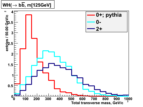
Figure 1: (color online) Transverse mass of the $\ell\nu b\bar{b}$ system for the $J^{P}=0^{+}$  $J^{P}=0^{-}$  and $J^{P}=2^{+}$ signals. These are shown after reconstruction for the two tight tag channel. The histograms are normalized to unit area.

3 Event Selection

We summarize the event selection for the $WH\rightarrow\ell\nu b\bar{b}$ channel. More details can be found in A. Abazov et al. $\!{}^{{\bf?}}$. We require one lepton ($\mu$ or $e$), large missing transverse energy ($\not\!\!E_{T}$), and two or three jets in the final state. We utilize b-tagging to identify the decay products of the SMS and divide the events into four orthogonal tagging categories: “one tight tag,” “two loose tags,” “two medium tags,” and “two tight tags.” A Boosted Decision Tree (BDT) is trained for each tagging category and jet multiplicity to separate SM signal from background.

4 Final Variable Distributions

In order to differentiate between the three spin-parity assignments we use the transverse mass of the $\ell\nu b\bar{b}$ system defined by

$$M_{T}^{2}=\left(E_{T}^{W}+E_{T}^{H}\right)^{2}-\left(\vec{p}_{T}^{W}+\vec{p}_{T}^{H}\right)^{2}$$ (1)

where the transverse momentum of the $W$ boson, $\vec{p}_{T}^{W}$, is defined as

$$\vec{p}_{T}^{W}=\vec{\mbox{$\not\!\!E_{T}$}}+\vec{p}_{T}^{\ell}$$ (2)

To illustrate the differences between the three hypotheses for this kinematic variable, the three signal hypotheses are shown in Fig. 1 after reconstruction. In addition to being able to differentiate between the test signals (i.e. the $J^{P}=0^{-}$ and $2^{+}$ signals), Fig. 2 shows the non-SM test signals peaking in a different region than either the SM signal or the other backgrounds. To ensure adequate background statistics when performing our statistical analysis, we rebin our $M_{T}$ distribution so that bins above $600$ GeV are included as a single overflow bin.

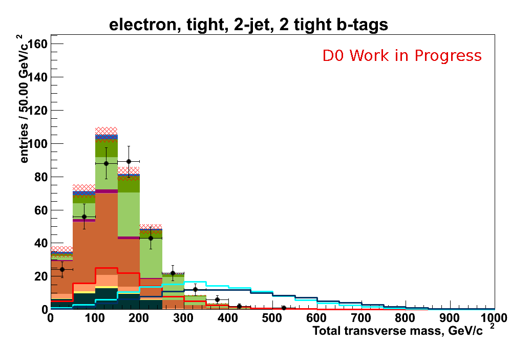
Figure 2: (color online) Transverse mass of the $\ell\nu b\bar{b}$ system with accompanying legend.

5 Statistical Interpretation

We use a modified frequentist (CL_S) approach with a log-likelihood ratio test statistic (LLR) for two hypotheses: the test hypothesis $H_{1}$ and the null hypothesis $H_{0}$. The LLR test statistic is given by

$$LLR=-2\ln\frac{L_{H_{1}}}{L_{H_{0}}}$$ (3)

where $L_{H_{x}}$ is the likelihood function for the hypothesis $H_{x}$. For a typical SMS search $H_{0}$ is the background-only hypothesis and $H_{1}$ is the signal plus background hypothesis. We can view our analysis through two different paradigms:

$\mathbf{H_{0}=b}$ and $\mathbf{H_{1}=s_{1}+b}$

here we decide if the data looks more like it came from a background-only distribution or from a test signal plus background distribution

$\mathbf{H_{0}=s_{0}+b}$ and $\mathbf{H_{1}=s_{1}+b}$

here we decide if our data looks more like it came from a SM signal plus background distribution or from a test signal plus background distribution

To gain insight on the separation significance we look at the LLR distributions populated by simulated experiments, assuming Poisson statistics, drawn from populations of the test and null hypotheses. As a preliminary result, we present the LLR distributions for the $J^{P}=2^{+}$ plus background hypothesis and background-only hypothesis for the $WH\rightarrow\ell\nu b\bar{b}$ channel (Fig. 3 (left)) and all $VH\rightarrow Vb\bar{b}$ channels combined (Fig. 3 (right)). The spatial separation between the signal plus background and background-only LLR distributions is a good illustration of how effective the analysis is at separating the signal plus background and the background-only hypotheses. From these LLR distributions it is clear then that we achieve good separation between the signal plus background vs. background-only hypotheses.

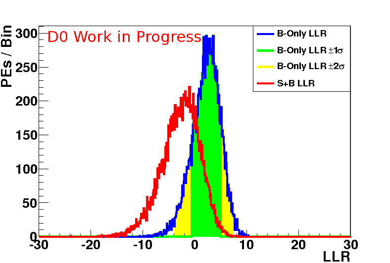
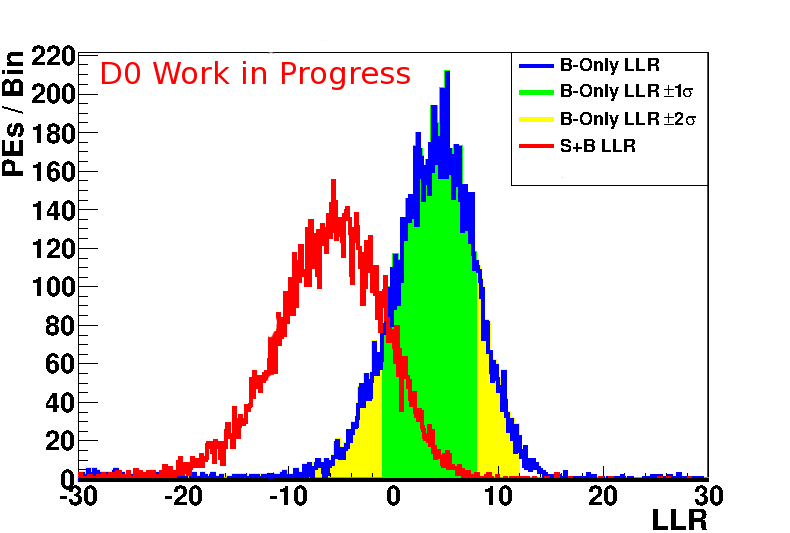
Figure 3: (color online) LLR distributions for the $WH\rightarrow\ell\nu b\bar{b}$ channel (left) and the combination of the $VH\rightarrow Vb\bar{b}$ channels (right) for the $J^{P}=2^{+}$ plus background and background-only hypotheses.

6 Summary

In summary, we presented preliminary results from the D0 experiment on the spin and parity of the newly observed SMS boson in the $WH\rightarrow\ell\nu b\bar{b}$ channel. While presently unable to show the observed LLR line, it is clear that we achieve good separation between the hypotheses.

References

References

- [1] P.W. Higgs, Phys. Lett. 12, 132 (1964).
- [2] F. Englert and R. Brout, Phys. Rev. Lett. 13, 321 (1964).
- [3] G. Aad et al., [ATLAS Collaboration], Phys. Lett. B 716, 1 (2012).
- [4] S. Chatrchyan et al., [CMS Collaboration], Phys. Lett. B 716, 30 (2012).
- [5] T. Aaltonen et al., [CDF and D0 Collaboration], Phys. Rev. Lett. 109, 071804 (2012).
- [6] L. Landau, Dokl.Akad.Nauk Ser.Fiz. 60, 207 (1948).
- [7] C.-N. Yang, Phys. Rev. 77, 242 (1950).
- [8] G. Aad et al., [ATLAS Collaboration], ATLAS-CONF-2013-040, (2013).
- [9] S. Chatrchyan et al., [CMS Collaboration], CMS-PAS-HIG-13-005, (2013).
- [10] J. Ellis, D.S. Hwang, V. Sanz, and T. You, J. High Energy Phys. 1211, 134 (2012).
- [11] V.M. Abazov et al., [D0 Collaboration], arXiv:1301.6122, (2013), accepted by Phys. Rev. D.
- [12] V.M. Abazov et al., [D0 Collaboration], Phys. Lett. B 716, 285 (2012).
- [13] V.M. Abazov et al., [D0 Collaboration], arXiv:1303.3276, (2013), accepted by Phys. Rev. D.
- [14] M.L. Mangano, F. Piccinini, A.D. Polosa, M. Moretti, and R. Pittau, J. High Energy Phys. 0307, 001 (2003).
- [15] T. Sjöstrand, S. Mrenna, and P. Skands, J.High Energy Phys. 0605, 026 (2006).
- [16] E.E. Boos, V.E. Bunichev, L.V. Dudko, V.I. Savrin, and V.V. Sherstnev, Phys. Atom. Nucl. 69, 1317 (2006).
- [17] J. Alwall, M, Herquet, F. Maltoni, O. Mattelaer, and T. Stelzer, J. High Energy Phys. 1106, 128 (2011).