The lengths of shortest non-contractible loops are studied numerically in 2d Euclidean quantum gravity on a torus coupled to conformal field theories with central charge less than one. We find that the distribution of these geodesic lengths displays a scaling in agreement with a Hausdorff dimension given by the formula of Y. Watabiki.

PACS: 04.60.Ds, 04.60.Kz, 04.06.Nc, 04.62.+v.
Keywords: quantum gravity, lower dimensional models, lattice models.

1 Introduction

The path integral plays an important role in quantum mechanics and quantum field theory. A feature of the path integral is that a “generic” path $X_{i}(t)$, $i=1,\ldots,d$, is fractal with Hausdorff dimension $D_{H}=2$. This is true irrespective of the dimension $d$ of space. The word “generic” refers to the path integral when rotated to imaginary time. When this is done one has a measure on the set of parametrized continuous paths, the Wiener measure, and with respect to this measure a randomly chosen continuous path has Hausdorff dimension 2. While the free non-relativistic particle is described by the path integral over parametrized paths in $d$ dimensions, the path integral for the free relativistic particle can be defined by considering paths in $D=d+1$ dimensional spacetime and use the Brink–Di Vechhia–Howe action for the particle, where one includes an intrinsic metric on the world line as a dynamical variable. The path integral can thus be viewed as the path integral of one-dimensional quantum gravity coupled to $D$ Gaussian fields $X_{\mu}$, the coordinates of space-time (see [1] for a review). Still, in this approach the Hausdorff dimension of the ensemble of paths in $D$ dimensions is two, while the dimension of the “intrinsic” parameter space trivially is one.

The generalization of the Brink–Di Vecchia–Howe action to strings leads to the Polyakov path integral. In this theory we have an intrinsic two-dimensional metric on the world sheet and coupled to this $D$ Gaussian fields $X_{\mu}$. In this case we formally define the path integral as follows

$$Z_{V}=\int{\cal D}[g]_{V}\int{\cal D}[X_{m}]_{{\rm cm}}\;\mbox{e}^{-\int d^{2}\xi\sqrt{g}\,g^{ab}\partial_{a}X_{\mu}\partial_{b}X_{\mu}},$$ (1)

where the integration is over two-dimensional geometries with fixed volume $V$ and where the subscript “cm” signifies that the center of mass of the string is fixed, i.e.

$$\int d^{2}\xi\sqrt{g(\xi)}=V,~{}~{}~{}~{}\int d^{2}\xi X_{\mu}(\xi)=0.$$ (2)

We note that one can in principle perform the Gaussian integration over the fields $X_{\mu}$ and one finds

$$Z_{V}\propto\int{\cal D}[g]_{V}\left(\det(-\Delta_{g})\right)^{-D/2},$$ (3)

where $\Delta_{g}$ is the Laplace operator in the geometry defined by the metric $g_{ab}$. Note that this expression allows us an to treat also non-integer values for $D$. The so-called extrinsic Hausdorff dimension $D_{H}$ is then defined by

$$\langle X^{2}\rangle_{V}\sim V^{2/D_{H}}$$ (4)

where

$$\langle X^{2}\rangle_{V}=\frac{1}{VZ_{V}}\int\!{\cal D}[g]_{V}\!\!\int\!{\cal D}[X_{m}]_{{\rm cm}}\;\mbox{e}^{-\int d^{2}\xi\sqrt{g}\,g^{ab}\partial_{a}X_{\mu}\partial_{b}X_{\mu}}\;\int d^{2}\xi\sqrt{g}\;X_{\mu}^{2}(\xi).$$ (5)

This definition, when applied to the particle where the integration is over $d\xi$ rather than $d^{2}\xi$, leads to $D_{H}=2$ as mentioned above. In the case of string theory one encounters tachyons when $D>1$, and the corresponding Liouville theory is ill defined. For $D\leq 1$ one obtains [2]

$$\langle X^{2}\rangle_{V}\sim\log^{2}V~{}~{}(D=1),~{}~{}~{}~{}~{}\langle X^{2}\rangle_{V}\sim\log V~{}~{}(D<1),$$ (6)

where there result for $D<1$ is obtained by analytic continuation as mentioned above, by formally considering the Gaussian theory as a conformal field theory with central charge $c=D\leq 1$. Thus $D_{H}=\infty$ for non-critical string theory.

However, contrary to the particle case, we can define a non-trivial intrinsic Hausdorff dimension. This dimension is natural and of interest when we view non-critical string theory as two-dimensional (Euclidean) quantum gravity coupled to some conformal theory with central charge $c<1$. For such a conformal field theory one does not in general have a natural definition of $D_{H}$ which refers explicitly to the Gaussian fields $X_{\mu}$, but we can, by analogy with (4), define the intrinsic Hausdorff dimension as

$$\langle r^{2}\rangle_{V}\sim V^{2/d_{h}}.$$ (7)

The average is defined with respect to the partition function $Z_{V}$:

$$Z_{V}=\int{\cal D}[g]_{V}Z_{V}(g,c),$$ (8)

where $Z(g,c)$ denotes the partition function for the conformal field theory with central charge $c$ we consider, in the “background geometry” defined by the 2d metric $g_{ab}(\xi)$. The functional integration in (8) is over two-dimensional geometries with volume $V$, as defined in eq. (2), and the average in (7) is now

$$\langle r^{2}\rangle_{V}=\frac{1}{2V^{2}Z_{V}}\int{\cal D}[g]Z_{V}(g,c)\int\!d^{2}\xi\!\int\!d^{2}\xi^{\prime}\sqrt{g(\xi)}\sqrt{g(\xi^{\prime})}\;r^{2}_{g}(\xi,\xi^{\prime})$$ (9)

where $r_{g}(\xi,\xi^{\prime})$ denotes the geodesic distance between $\xi$ and $\xi^{\prime}$ in the geometry defined by $g_{ab}(\xi)$.

A remarkable formula for $d_{h}$ was derived by Y. Watabiki [3], using Liouville theory and the heat kernel expansion:

$$d_{h}^{W}(c)=2\,\frac{\sqrt{49-c}+\sqrt{25-c}}{\sqrt{25-c}+\sqrt{1-c}}.$$ (10)

This formula is not the only one proposed. Already in the original articles where quantum Liouville theory was defined an alternative formula was suggested [4]

$$d_{h}^{\prime}=-\frac{2}{\gamma},~{}~{}~{}\gamma=\frac{c-1-\sqrt{(1-c)(25-c)}}{12}.$$ (11)

The two formulas agree for $c=0$ where $d_{h}^{W}=d_{h}^{\prime}=4$. However, they have a quite different behavior for $c\to-\infty$ where $d_{h}^{\prime}\to 0$ while $d_{h}^{W}\to 2$. Formally one expects $d_{h}\to 2$ since this is the limit where the quantum Liouville theory should behave semiclassically and matter and geometry should be only weakly coupled, and this is indeed the behavior of $d_{h}^{W}$. On the other hand it is quite difficult to provide any geometric interpretation of $d_{h}^{\prime}\to 0$. The difference between the two predictions becomes even more pronounced when we consider the region $0<c<1$. For $c\to 1$ $d_{h}^{\prime}\to\infty$ while $d_{h}^{W}\to 2+2\sqrt{2}=4.83$.

That the value $d_{h}=4$ is correct for $c=0$ has been proven in [5, 6]. The present understanding is that $d_{h}^{\prime}$ does not reflect the behavior (7) with $r$ being the geodesic distance when $c\neq 0$. Rather it reflects the behavior of some structures related to matter. This is nicely exemplified for $c=1/2$. The continuum $c=1/2$ theory in flat spacetime can be obtained as the scaling limit of the Ising model defined on a regular 2d lattice. The Ising model has a critical temperature (or coupling constant) and a second order phase transition where one can define the $c=1/2$ conformal field theory. Similarly the continuum 2d quantum gravity theory coupled to a $c=1/2$ conformal field theory can be obtained as the scaling limit of an Ising model coupled to so-called “dynamical” triangulations [7], i.e. rather than considering the Ising model on a fixed regular lattice, one considers the Ising model on lattices with fixed 2d topology, but otherwise random connectivity, and sums over all such random lattices. If we compare with formula (8) the number of vertices can (scaled suitably) be identified with $V$, the sum over geometries can be identified with the sum over lattices with different connectivities (and it can all be made quite precise using the formalism of dynamical triangulations (DT), see [1] for a review). The Ising model on this so-called annealed average of lattices still has a critical point and a corresponding phase transition where the continuum limit can be obtained. The critical exponents one finds in this limit are precised the KPZ exponents of a $c=1/2$ theory coupled to 2d quantum gravity. For $c=1/2$ one obtains $d_{h}^{\prime}=6$. The seminal work of Kawai and Ishibashi [8] shows that one obtains $d_{h}=6$ in the DT Ising model, not by using the geodesic distance (for instant the shortest link distance between two vertices), but by counting the number of spin boundaries separating the two vertices. Of course it might be that for large volumes the average number of spin boundaries separating two vertices is proportional to the average number of links separating the vertices. However, computer simulations do not support this, but suggest that the geometric Hausdorff dimension is closer to the value $d_{h}^{W}(c=1/2)=4.21$ suggested by the Watabiki formula.

Almost the same story can be repeated for $c=-2$ theories. In this case $d_{h}^{W}=3.562$ while $d^{\prime}_{h}=2$. Analytically it is possible to obtain the $d^{\prime}_{h}$ value [9] from a specific discretized theory, the $O(n)$ model coupled to DT, where the value $n=-2$ corresponds to $c=-2$, but again this value is obtained by using in (7) an $r$ with no direct relation to the geometric distances on DT lattices but rather to spin boundaries in the $O(n)$ model. On the other hand it is formally possible to realize the $c=-2$ model on dynamical triangulations if one uses the Polyakov string partition function (3) analytically continued to $D=-2$ fields. Remarkably, it is possible to find an algorithm which generates the triangulations recursively with the correct weight in this case [10], allowing one to numerically determine the geometric $d_{h}$ for very large triangulations [11]. One finds perfect agreement with the Watabiki formula. Recently, measurements of the geometric $d_{h}$ have been performed for large negative $c$, based on Monte Carlo simulations using the partition function (3), again analytically continued to large negative $D$. One observes agreement with the Watabiki formula [12]. Also, one observes (at a qualitative, visual level [12]) that the typical geometries generated in the computer simulations become less fractal for large negative $D$ in accordance with the expectation that smooth geometries should dominate in the $c=-\infty$ limit in the Liouville theory. This is probably the reason it is possible at all to determine $d_{h}$ numerically for large negative $D$ using (3), since the presence of the determinant for numerical reasons constraints the size of the triangulations (except for $D=-2$).

It is thus fair to say there is good “empirical” evidence that (10) is the geometric Hausdorff dimension for $c\leq 0$. The purpose of this article is to test numerically whether (10) is valid also in the range $0<c<1$. Why is this needed? One should keep in mind that the analytic arguments which led to (10) are not rigorous arguments, as emphasized by Watabiki himself [3]. They rely on the interchangeability of certain limits when averaging over geometries and averaging over diffusion-paths, which is not necessarily true. It might be true for $c\leq 0$ but not for $c>0$ where the average geometry could become more fractal. In fact there is distinction between the regions $c<0$ and $c>0$. For minimal conformal theories with $c>0$ coupled to 2d gravity the dominant infrared coupling constant is the cosmological coupling constant, while for $c<0$ one has primary fields of negative dimensions and the coupling constant related to the primary operator of the most negative dimension is expected to dominate the infrared in an effective field theory. We do not presently understand how such a dominance is transferred to a change of $d_{h}$, but if that is the case one could have a scenario where $d_{h}$ varies for $c<0$ (and agrees with (10)), while it stays 4 for $c>0$. In fact, the Monte Carlo simulations performed prior to the present work (see [18, 19] and in particular [20]) have not been precise enough to settle the question whether $d_{h}$ remains 4 for $c>0$ or whether it changes according to (10) as a function of $c$. In particular the most extensive simulations performed so far, rapported in [20], were agonizing since the results seemed to depend on the observable one used. Finite size analysis using the spin correlators seemed to favor $d^{W}_{h}(c)$ although with somewhat large error bars, while the use of geometric quantity favored the $d_{h}=4$ hypothesis for $c\geq 0$. Recently arguments have been given [15] in favor of $d_{h}=4$.

In this article we will provide a new method for measuring $d_{h}$ based on 2d geometries with toroidal topology. The method allows us to measure $d_{h}$ with high precision and leads to agreement with $d^{W}_{h}(c)$ given by (10) also for $0<c<1$. To be precise, we will show that $d_{h}^{W}(c)$ describes the fractal geometry for two unitary matter systems coupled to 2d quantum gravity, namely the $c=1/2$ and $c=4/5$ conformal field theories. Until now formula (10) has only been verified convincingly for $c=0$ and (numerically) for the somewhat artificial, analytic continuation of (3) to negative $D$.

2 Measuring the toroidal Hausdorff dimension

2.1 The set up

As described above we expect geodesic distances to scale anomalously in 2d Euclidean quantum gravity. In [12, 13, 14] this was used to measure $d_{h}$ for spacetimes with toroidal topology. The basic observation was that a shortest non-contractible loop (if it exists) is a geodesic curve. Let the intrinsic Hausdorff dimension be $d_{h}$, let the spacetime volume be $V$ and let the probability distribution of the shortest non-contractible loop be $P_{V}(L)$. Since $x=L/V^{1/d_{h}}$ is dimensionless and so is $P(L)dL$, we expect a relation

$$P_{V}(L)=V^{-1/d_{h}}F(x),$$ (12)

where the function $F(x)$ contains no dependence of $V$ except the one found in $x$. From (12) one obtains that $\langle L\rangle\sim V^{1/d_{h}}$ and it was this scaling relation which was used in [12, 13, 14] to determine $d_{h}$. Here we will directly use relation (12) to determine $d_{h}$.

If we regularize 2d quantum gravity using DT, the relation (12) can be read as a standard finite size scaling relation, using the terminology from the theory of critical phenomena. The volume $V$ is replaced by the number of triangles $N$ in the triangulation, a loop consists of links and $L$ is replaced by number of links $\ell$ in the shortest non-contractible loop for the given triangulation. Finally, the probability distribution $P_{V}(L)$ refers to the distribution obtained for the ensemble of toroidal geometries for a quantum gravity theory with the partition function (8). In the regularized setting of DT the conformal field theory with central charge $c$ is represented in some way. As an example, the Ising model can be represented by Ising spins on the triangles, interacting with the spins on the neighboring triangles, and the (inverse) temperature $\beta$ put equal to the critical value $\beta_{c}$ to ensure the Ising model represents a $c=1/2$ conformal field theory. In such a theory we can determine $P_{N}(\ell)$ numerically by generating a large number of independent triangulations (with the weight of matter taken into account) and then simply measure the shortest non-contractible loop for each configuration. Eq. (12) is then replaced by the finite size scaling relation

$$P_{N}(\ell)=N^{-1/d_{h}}F(x),~{}~{}~{}~{}x=\frac{\ell}{N^{1/d_{h}}}.$$ (13)

By measuring $P_{N}(\ell)$ for different $N$ we will can easily test if the scaling assumption is satisfied and determine by standard fitting the best value of $d_{h}$. Of course we cannot expect (13) to be valid and reproduce a continuum formula like (12) for small values of $N$, so usually the fitting procedure will also involve discarding some range of small $N$.

The length of a shortest non-contractible loop is just the first of a sequence of natural geodesic lengths, $0<\ell_{1}\leq\ell_{2}\leq\cdots$ that one can assign to a torus. These $\ell_{i}$ are defined in the following way. First one notices that the closed curves on a torus fall into homotopy classes. In the piecewise linear geometries like the ones generated by DT, these classes contain the closed paths consisting of sequences of edges that can be deformed into eachother with local deformations. We call a homotopy class simple if it contains a simple curve, i.e. a curve which does not intersect itself. In each non-trivial simple homotopy class $\Gamma$ we can find one or more paths which have a minimum length $\ell_{\Gamma}$ and which can regarded as discrete geodesics. If we order the lengths $\ell_{\Gamma}$ for all $\Gamma$ we obtain a well-defined sequence of lengths

$$0<l_{1}\leq l_{2}\leq\cdots$$ (14)

and a corresponding sequence of probability distributions:

$$P_{N}^{(i)}(\ell_{i})=N^{-1/d_{h}}F_{i}\Big{(}\ell_{i}/N^{1/d_{h}}\Big{)}.$$ (15)

It turns out to be advantageous to use $P_{N}^{(2)}(\ell_{2})$ in the determination of $d_{h}$. In average $\ell_{2}$ will be larger than $\ell_{1}$ (see Fig. (2) below) and the resulting probability distribution is significantly less sensitive to finite size effects. We do not fully understand why this is so, but it makes it worth to construct $P_{N}^{(2)}(\ell_{2})$, even if it is more computer-demanding to find $\ell_{2}$.

In [13] we described an algorithm which allows one to find $\ell_{1}$ and the corresponding loop $\gamma_{1}$ efficiently for large triangulations. To find $\ell_{2}$ we are looking for a simple closed path $\gamma_{2}$ of minimal length which is neither homotopic to $\gamma_{1}$ nor to a point. This implies that it has to intersect $\gamma_{1}$ at least once. Therefore we can find $\gamma_{2}$ by performing for each vertex in $\gamma_{1}$ a search starting at that vertex in the following way. First we inspect the neighbors of the starting vertex, then the neighbors of the neighbors, etc. Encountering a vertex that has been visited before means that one has discovered a loop in the triangulation. We stop at the first such loop which is neither homotopic to $\gamma_{1}$ nor to a point. It is not hard to see that the length of this loop is the sought-after length $\ell_{2}$. Examples of the curves $\gamma_{1}$ and $\gamma_{2}$ for a large random triangulation $T$ are shown in Fig. 1.

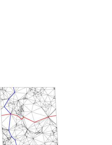
Figure 1: A random triangulation of the torus coupled to Ising spins. The thick red curve is a shortest non-contractible loop of length $\ell_{1}=6$, while the thick blue curve is the “second shortest” loop of length $\ell_{2}=7$. The embedding of the triangulation in a parallelogram in the complex plane is constructed using the methods in [14].

2.2 The numerical results

We use the method described above to determine $d_{h}$ for $c=-2,0,1/2$ and 4/5. For $c=-2$ and 0 we have already determined $d_{h}$ with good precision measuring $\langle\ell_{1}\rangle$ corresponding to the distributions $P_{N}^{(1)}(\ell_{1})$, so the determination of $d_{h}$ for these values of $c$ using finite size scaling directly on the distribution $P_{N}^{(2)}(\ell_{2})$ is basically a check that the method works. The triangulations are generated as described in [13, 14] by Monte Carlo simulations for $c=0$ and by a recursive algorithm for $c=-2$. The class of triangulations used is the most general one where links in a triangle are allowed to be identified and where pairs of triangles are allowed to share more than one edge. The $c=1/2$ system is realized as Ising spins on the triangles, interacting with spins on neighboring triangles. The $c=4/5$ system is realized as a 3-states Potts model, the spins also on the triangles. For a fixed triangulation the partition function takes the form

$$Z_{Q}=\sum_{\sigma\in\{1,\ldots,Q\}^{N}}\exp\left(2\beta_{Q}\sum_{\langle ij\rangle}\delta_{\sigma_{i}\sigma_{j}}\right),$$ (16)

with $Q=2$ for the Ising spins and $Q=3$ for the 3-states Potts model. The sum in the exponential is over the pairs of adjacent triangles $i$ and $j$. The coupling constants $\beta_{Q}$ are chosen to be the critical coupling in the infinite volume limit (i.e. the $N\to\infty$ limit). For the general ensemble of triangulations used here, and with the spins on the triangles these are known: $\beta_{2}=1/2\log(1+2\sqrt{7})\approx 0.9196$ and $\beta_{3}=1/2\log(1+\sqrt{47})\approx 1.0306$ (see [16] and [17, 18] respectively). The updating of the triangulations is done in the standard way by flipping the diagonal of a randomly selected pair of adjacent triangles. The Wolff algorithm [23] is used to efficiently update the spins at the critical points.

The simulations were performed with triangulations of the torus with $N=250$ up to $N=256000$ triangles. First the systems were thermalized by performing roughly $10^{5}$ sweeps, where a sweep corresponds to on average $N$ random update moves on the triangulation and $N$ spin flips. After thermalization between $10^{5}$ and $10^{6}$ measurements of $\ell_{1}$ and $\ell_{2}$ were performed with 100 sweeps in between measurements. From the measurements one can construct the probability distribution $P_{N}^{(i)}(\ell_{i})$ for obtaining a particular length $\ell_{i}$ for a random triangulation with $N$ triangles, as shown in figure 2 for $N=8000$.

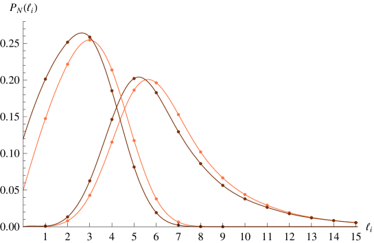
Figure 2: The probability distributions $P_{N}^{(i)}(\ell_{i})$, $i=1,2$, for dynamical triangulations coupled to the Ising model (light points) and coupled to the Potts model (dark points). The curves are smooth interpolations used for finding the scaling. The left curves are $P_{N}^{(1)}(\ell_{1})$ and the right curves are $P_{N}^{(2)}(\ell_{2})$, all for $N=8000$

To study the finite size scaling we fit $P_{N}^{(2)}(\ell_{2})\propto f(k\ell_{2})$, where $f(\tilde{\ell}_{2})$ is a smooth interpolation of the distribution $P_{N=8000}^{(2)}(\ell_{2})$ obtained for $N=8000$ triangles. When performing the fit for a fixed $N$ we took into account only the data points for which $P_{N}(\ell_{2})$ was larger than $0.1$ times the largest $P_{N}(\ell_{2})$. We made this choice based on the fact that the collapse of the $P_{N}(\ell_{2})$ for different $N$ according to (13) is very accurate for the peak of the distribution but less so for its tail at large $\ell_{2}$. One may view the values of $k$ obtained by such a best fit to be an accurate measurement of (the inverse of) the position of the peak in the distribution $P_{N}(\ell_{2})$. The results of the best fits for $k$ as function of $N$ are shown in figure 3. We have rescaled $k$ by $(N/8000)^{1/4}$, such that a flat curve would correspond to $k\propto N^{-1/4}$. By construction the points for $N=8000$ take the value $1$. On the figure we have also shown the data for $c=0$ and $c=-2$ as described above.

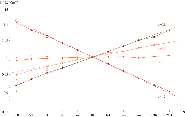
Figure 3: The values $k$ leading to a best fit $P_{N}^{(2)}(\ell_{2})\propto f(k\ell_{2})$, where $f(\tilde{\ell}_{2})$ is the smooth interpolation of $P_{N=8000}^{(2)}(\ell_{2})$ shown in figure 2. The shown errors are predominantly systematic, as a result of the fact that the profiles $P_{N}^{(2)}(\ell_{2})$ do not exactly collapse. The dash lines correspond to $k\propto N^{-1/d_{h}^{W}}$ with $d_{h}^{W}$ the values given by formula (10).

The fitted values $k$ show a beautiful scaling with the volume $N$ and are in agreement with $k\propto N^{-1/d_{h}^{W}}$ with $d_{h}^{W}$ given by formula (10), as indicated by the dash lines. Extracting the slopes by a fit one obtains the values in the following table, which are also plotted in figure 4.

$c$	$d_{h}$ (by fit)	$d_{h}$ (theoretical)
$-2$	$3.575\pm 0.003$	$3.562$
$0$	$4.009\pm 0.005$	$4.000$
$1/2$	$4.217\pm 0.006$	$4.212$
$4/5$	$4.406\pm 0.007$	$4.421$

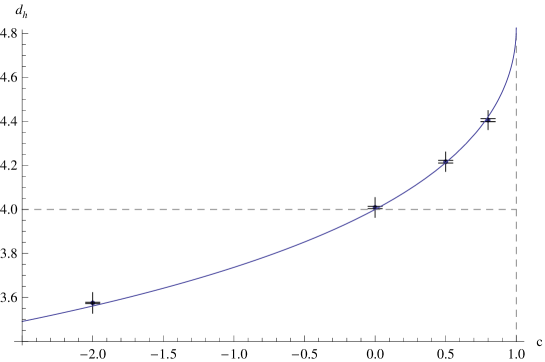
Figure 4: The values for the Hausdorff dimension $d_{h}$ as extracted from the slope of the curves in figure 3. The curve corresponds to formula (10).

3 Discussion

As seen from the table above and Fig. 4 the agreement between formula (10) and the values of $d_{h}(c)$ is impressive, in particular when one compares to the precision one could obtain using the older methods for extracting $d_{h}$. Our present measurements provide convincing numerical evidence that the peak in the distribution of second shortest loop lengths scales according to a Hausdorff dimension given by the Watabiki formula (10). It is interesting to compare in more detail with results obtained in [20], where the Hausdorff dimension was extracted for spacetimes with spherical topologies, using two-point correlation functions, either entirely geometric or spin-spin correlation functions. Finite size scaling analysis applied to the spin-spin correlation functions the same way as finite size scaling has been applied in this article led to agreement with $d_{h}^{W}(c)$, although with large errorbars. However, the finite size scaling applied to geometric correlators and expectation values, as well as the study of the short distance part of the correlators, spin or geometric, led to better agreement with $d_{h}(c)=4$ for $0\leq c<1$.

In this article we have only been looking at geometric quantities and we have for the first time seen that they scale according to $d_{h}^{W}(c)$ for $c>0$, even quite convincingly, with significantly smaller error bars than were present in measurement of geometric corelators in the work [20]. Does that rule out the $d_{h}(c)=4$ hypothesis for $0\leq d_{h}\leq 1/4$? Not entirely. As mentioned above, we obtained the clean scaling results by cutting away the tales of the distributions $P_{N}^{(2)}(\ell_{2})$ (we imposed $P_{N}^{(2)}(\ell_{2})\geq 0.1\,\max(P_{N}^{(2)}(\ell_{2}))$). In fact, preliminary investigation of the tail of the distribution has shown that the decay of $P_{N}^{(2)}(\ell_{2})$ for large $\ell_{2}$ is approximately exponential and that the decay rate scales more like $N^{-1/4}$ than $N^{-1/d_{h}^{W}}$. However, more statistics and larger system sizes are required to decide the matter.

Acknowledgments. The authors acknowledge support from the ERC-Advance grant 291092, “Exploring the Quantum Universe” (EQU). JA acknowledges support of FNU, the Free Danish Research Council, from the grant “quantum gravity and the role of black holes”. Finally this research was supported in part by the Perimeter Institute of Theoretical Physics. Research at Perimeter Institute is supported by the Government of Canada through Industry Canada and by the Province of Ontario through the Ministry of Economic Development & Innovation.

References

- [1] J. Ambjorn, B. Durhuus and T. Jonsson, Cambridge, UK: Univ. Pr., 1997. (Cambridge Monographs in Mathematical Physics). 363 p
- [2] J. Ambjorn, D. Boulatov, J. L. Nielsen, J. Rolf and Y. Watabiki, JHEP 9802 (1998) 010 [hep-th/9801099].
- [3] Y. Watabiki, Prog. Theor. Phys. Suppl. 114 (1993) 1-17.
- [4] J. Distler, Z. Hlousek, H. Kawai, Int. J. Mod. Phys. A 5 (1990) 1093.
- [5] H. Kawai, N. Kawamoto, T. Mogami, Y. Watabiki, Phys. Lett. B 306 (1993) 19-26 [hep-th/9302133].
- [6] J. Ambjørn, Y. Watabiki, Nucl. Phys. B 445 (1995) 129-144 [hep-th/9501049].
- [7] V. A. Kazakov, Phys. Lett. A 119 (1986) 140-144.
- [8] N. Ishibashi and H. Kawai, Phys. Lett. B 322 (1994) 67 [hep-th/9312047].
- [9] J. Ambjørn, K.N. Anagnostopoulos, J. Jurkiewicz, C.F. Kristjansen, JHEP 9804 (1998) 016 [hep-th/9802020].
- [10] N. Kawamoto, V.A. Kazakov, Y. Saeki, Y. Watabiki, Phys. Rev. Lett. 68 (1992) 2113-2116.
- [11] J. Ambjørn, K.N. Anagnostopoulos, T. Ichihara, L. Jensen, N. Kawamoto, Y. Watabiki, K. Yotsuji, Phys. Lett. B 397 (1997) 177-184 [hep-lat/9611032]; Nucl. Phys. B 511 (1998) 673-710 [hep-lat/9706009].
- [12] J. Ambjorn and T. G. Budd, Phys. Lett. B 718 (2012) 200 [arXiv:1209.6031 [hep-th]].
- [13] J. Ambjorn, J. Barkley, T. Budd and R. Loll, Phys. Lett. B 706 (2011) 86 [arXiv:1110.3998 [hep-th]].
- [14] J. Ambjorn, J. Barkley and T. G. Budd, Nucl. Phys. B 858 (2012) 267 [arXiv:1110.4649 [hep-th]].
- [15] B. Duplantier, arXiv:1108.3327 [math-ph].
- [16] D. V. Boulatov, V. A. Kazakov, Phys. Lett. B 186 (1987) 379.
- [17] J.-M. Daul, hep-th/9502014.
- [18] S. Catterall, G. Thorleifsson, M. Bowick, V. John, Phys. Lett. B 354 (1995) 58 [hep-lat/9504009].
- [19] J. Ambjorn, J. Jurkiewicz, Y. Watabiki, Nucl. Phys. B 454 (1995) 313 [hep-lat/9507014].
- [20] J. Ambjorn and K. N. Anagnostopoulos, Nucl. Phys. B 497 (1997) 445 [hep-lat/9701006].
- [21] E. Guitter, J. Stat. Mech. (2010) P04018 [arXiv:1003.0372 [math-ph]].
- [22] T. Jonsson, Phys. Lett. B 425 (1998) 265 [hep-th/9801150].
- [23] U. Wolff, Phys. Rev. Lett. 62 (1989) 361.