Topological entropy of quadratic polynomials and dimension of sections of the Mandelbrot set

Abstract.

Let $c$ be a real parameter in the Mandelbrot set, and $f_{c}(z):=z^{2}+c$. We prove a formula relating the topological entropy of $f_{c}$ to the Hausdorff dimension of the set of rays landing on the real Julia set $J(f_{c})\cap\mathbb{R}$, and to the Hausdorff dimension of the set of rays landing on the real section of the Mandelbrot set, to the right of the given parameter $c$. We then generalize the result by looking at the entropy of Hubbard trees: namely, we relate the Hausdorff dimension of the set of external angles which land on a certain slice of a principal vein in the Mandelbrot set to the topological entropy of the quadratic polynomial $f_{c}$ restricted to its Hubbard tree.

1. Introduction

Let us consider the family of quadratic polynomials

$$f_{c}(z):=z^{2}+c,\quad\textup{with }c\in\mathbb{C}.$$

The filled Julia set $K(f_{c})$ of a quadratic polynomial $f_{c}$ is the set of points which do not escape to infinity under iteration, and the Julia set $J(f_{c})$ is the boundary of $K(f_{c})$. The Mandelbrot set $\mathcal{M}$ is the connectedness locus of the quadratic family, i.e.

$$\mathcal{M}:=\{c\in\mathbb{C}\ :\ \textup{ the Julia set of }f_{c}\textup{ is connected}\}.$$

A fundamental theme in the study of parameter spaces in holomorphic dynamics is that the local geometry of the Mandelbrot set near a parameter $c$ reflects the geometry of the Julia set $J(f_{c})$, hence it is related to dynamical properties of $f_{c}$. In this paper we will establish an instance of this principle, by looking at the Hausdorff dimension of certain sets of external rays.

Recall that a measure of the complexity of a continuous map is its topological entropy, which is essentially defined as the growth rate of the number of itineraries under iteration (see section 5).

In our case, the map $f_{c}(z)=z^{2}+c$ is a degree-two ramified cover of the Riemann sphere $\hat{\mathbb{C}}$, hence a generic point has exactly $2$ preimages, and the topological entropy of $f_{c}$ always equals $\log 2$, independently of the parameter [Ly]. If $c$ is real, however, then $f_{c}$ can also be seen as a real interval map, and its restriction to the real line also has a well-defined topological entropy, which we will denote by $h_{top}(f_{c},\mathbb{R})$. The dependence of $h_{top}(f_{c},\mathbb{R})$ on $c$ is much more interesting: indeed, it is a continuous, decreasing function of $c$ [MT], and it is constant on baby Mandelbrot sets [Do3] (see Figure 1).

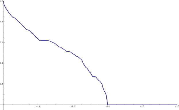
Figure 1. Topological entropy of the real quadratic family $f_{c}(z):=z^{2}+c$, as a function of $c$. For each value of $c\in[-2,-1]$, we plot the growth number $e^{h_{top}(f_{c})}$.

The Riemann map $\Phi_{M}:\hat{\mathbb{C}}\setminus\overline{\mathbb{D}}\to\hat{\mathbb{C}}\setminus\mathcal{M}$ uniformizes the exterior of the Mandelbrot set, and images of radial arcs are called external rays. Each angle $\theta\in\mathbb{R}/\mathbb{Z}$ determines the external ray $R_{M}(\theta):=\Phi_{M}(\rho e^{2\pi i\theta})_{\{\rho>1\}}$, which is said to land if the limit as $\rho\to 1^{+}$ exists.

Given a subset $A$ of $\partial{\mathcal{M}}$, one can define the harmonic measure $\nu_{M}$ as the probability that a random ray from infinity lands on $A$:

$$\nu_{M}(A):=\textup{Leb}(\{\theta\in S^{1}\ :\ R_{M}(\theta)\textup{ lands on }A\}).$$

If one takes $A:=\partial\mathcal{M}\cap\mathbb{R}$ to be the real slice of the boundary of $\mathcal{M}$, then the harmonic measure of $A$ is zero. However, the set of rays which land on the real axis has full Hausdorff dimension [Za]. (By comparison, the set of rays which land on the main cardioid has zero Hausdorff dimension.) As a consequence, it is more useful to look at Hausdorff dimension than harmonic measure; for each $c$, let us consider the section

$$P_{c}:=\{\theta\in S^{1}:R_{M}(\theta)\textup{ lands on }\partial{\mathcal{M}}\cap[c,1/4]\}$$

of all parameter rays which land on the real axis, to the right of $c$. The function

$$c\mapsto\textup{H.dim }P_{c}$$

increases from $0$ to $1$ as $c$ moves towards the tip of $\mathcal{M}$, reflecting the increased “hairiness” near the tip. In the dynamical plane, one can consider the set of rays which land on the real slice of $J(f_{c})$, and let $S_{c}$ be the set of external angles of rays landing on $J(f_{c})\cap\mathbb{R}$. This way, we construct the function $c\mapsto\textup{H.dim }S_{c}$, which we want to compare to the Hausdorff dimension of $P_{c}$.

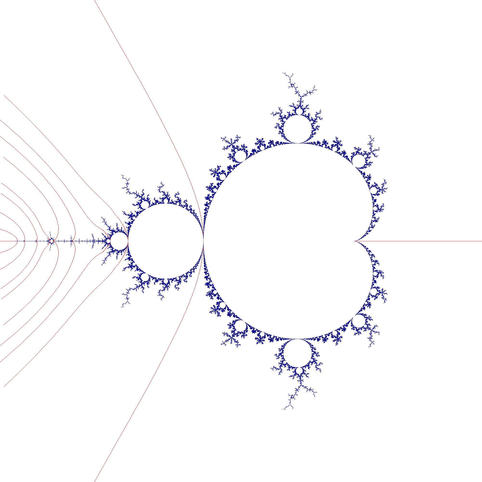
Figure 2. A few rays which land on the real slice of the Mandelbrot set.

The main result is the following identity:

Theorem 1.1.

Let $c\in[-2,1/4]$. Then we have

$$\frac{h_{top}(f_{c},\mathbb{R})}{\log 2}=\textup{H.dim }S_{c}=\textup{H.dim }P_{c}.$$

The first equality establishes a relation between entropy, Hausdorff dimension and the Lyapunov exponent of the doubling map (in the spirit of the “entropy formulas” [Ma], [Yo], [LeYo]), while the second equality can be seen as an instance of Douady’s principle relating the local geometry of the Mandelbrot set to the geometry of the corresponding Julia set. Indeed, we can replace $P_{c}$ with the set of angles of rays landing on $[c,c+\epsilon]$ in parameter space, as long as $[c,c+\epsilon]$ does not lie in a tuned copy of the Mandelbrot set. Note that the set of rays which possibly do not land has zero capacity, hence the result is independent of the MLC conjecture.

A first study of the dimension of the set of angles of rays landing on the real axis has been done in [Za], where it is proven that the set of angles of parameter rays landing on the real slice of $\mathcal{M}$ has dimension $1$. Zakeri also provides estimates on the dimension along the real axis, and specifically asks for dimension bounds for parameters near the Feigenbaum point ($-1.75\leq c\leq c_{Feig}$, see [Za], Remark 6.9). Our result gives an identity rather than an estimate, and the dimension of $S_{c}$ can be exactly computed in the case $c$ is postcritically finite (see following examples).

Recall the dimension of $S_{c}$ also equals the dimension of the set $B_{c}$ of angles landing at biaccessible points (Proposition 6.1). Smirnov [Sm] first showed that such set has positive Hausdorff dimension for Collet-Eckmann maps. More recent work on biaccessible points is due, among others, to Zakeri [Za2] and Zdunik [Zd]. The first equality in Theorem 1.1 has also been established independently by Bruin-Schleicher [BS].

A precise statement of the asymptotic similarity between $\mathcal{M}$ and Julia sets near Misiurewicz points is proven in [TanL].

Examples

1. If $c=0$, then $f^{n}_{c}(z)=z^{2^{n}}$ has only one lap for each $n$, hence the entropy is zero. Moreover, the characteristic ray is $\theta=0$, hence $P_{c}$ consists of only one element and it has zero dimension. Moreover, the Julia set is a circle and the set of rays landing on the real axis $S_{c}=\{0,\frac{1}{2}\}$ consists of two elements, hence the dimension is $0$.

2. If $c=-2$, then $f_{c}$ is a 2-1 surjective map from $[-2,2]$ to itself, hence the entropy is $\log 2$. The Julia set is a real segment, hence all rays land on the real axis and the Hausdorff dimension of $S_{c}$ is $1$. Similarly, the set of rays $P_{c}$ is the set of all parameter rays which land on the real axis, which has Hausdorff dimension $1$.

3. The basilica map $f_{c}(z)=z^{2}-1$ has a superattracting cycle of period $2$, and for each $n$, $f_{c}^{n}$ has $2n+1$ critical points, hence the entropy is $\lim_{n\to\infty}\frac{\log(2n+1)}{n}=0$. The angles of rays landing on the Hubbard tree are $\theta=\frac{1}{3},\frac{2}{3}$, and the set of rays landing on the real Julia set is countable, hence it has dimension $0$. In parameter space, the only rays which land on the real axis to the right of $c=-1$ are $\theta=0,1/3,2/3$, hence their dimension is still zero.

4. The airplane map has a superattracting cycle of period $3$, and its characteristic angle is $\theta_{c}=\frac{3}{7}$. The set of angles whose rays land on the Hubbard tree is the set of binary numbers with expansion which does not contain any sequence of three consecutive equal symbols. It is a Cantor set which can be generated by the automaton in Figure 3, and its Hausdorff dimension is $\log_{2}\frac{\sqrt{5}+1}{2}$.

   

   

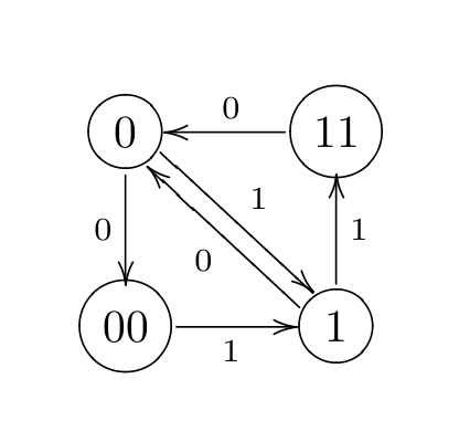
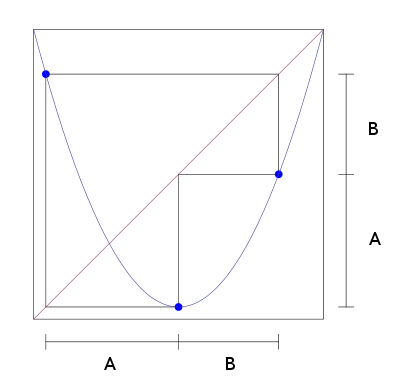
   Figure 3. To the right: the combinatorics of the airplane map of period $3$. To the left: the automaton which produces all symbolic orbits of points on the real slice of the Julia set.

   On the other hand, the topological dynamics of the real map is encoded by the right-hand side diagram: the interval $A$ is mapped onto $A\cup B$, and $B$ is mapped onto $A$. Then the number of laps of $f_{c}^{n}$ is given by the Fibonacci numbers, hence the topological entropy is the logarithm of the golden mean. It is harder to characterize explicitly the set of parameter rays which land on the boundary of $\mathcal{M}$ to the right of the characteristic ray: however, as a consequence of Theorem 1.1, the dimension of such set is also $\log_{2}\frac{\sqrt{5}+1}{2}$.

A more complicated example is the Feigenbaum point $c_{Feig}$, the accumulation point of the period doubling cascades. As a corollary of Theorem 1.1, we are able to answer a question of Zakeri ([Za], Remark 6.9):

Corollary 1.2.

The set of biaccessible angles for the Feigenbaum parameter $c_{Feig}$ has dimension zero:

$$\textup{H.dim }B_{c_{Feig}}=0.$$

1.1. The complex case

The result of Theorem 1.1 lends itself to a natural generalization for complex quadratic polynomials, which we will now describe.

In the real case, we related the entropy of the restriction of $f_{c}$ on an invariant interval to the Hausdorff dimension of a certain set of angles of external rays landing on the real slice of the Mandelbrot set.

In the case of complex quadratic polynomials, the real axis is no longer invariant, but we can replace it with the Hubbard tree $T_{c}$ (see section 4). In particular, we define the polynomial $f_{c}$ to be topologically finite if the Julia set is connected and locally connected and the Hubbard tree is homeomorphic to a finite tree (see Figure 4, left). We thus define the entropy $h_{top}(f_{c}\mid_{T_{c}})$ of the restriction of $f_{c}$ to the Hubbard tree, and we want to compare it to the Hausdorff dimension of some subset of parameter space. Let $H_{c}$ be the set of external rays which land on $T_{c}$.

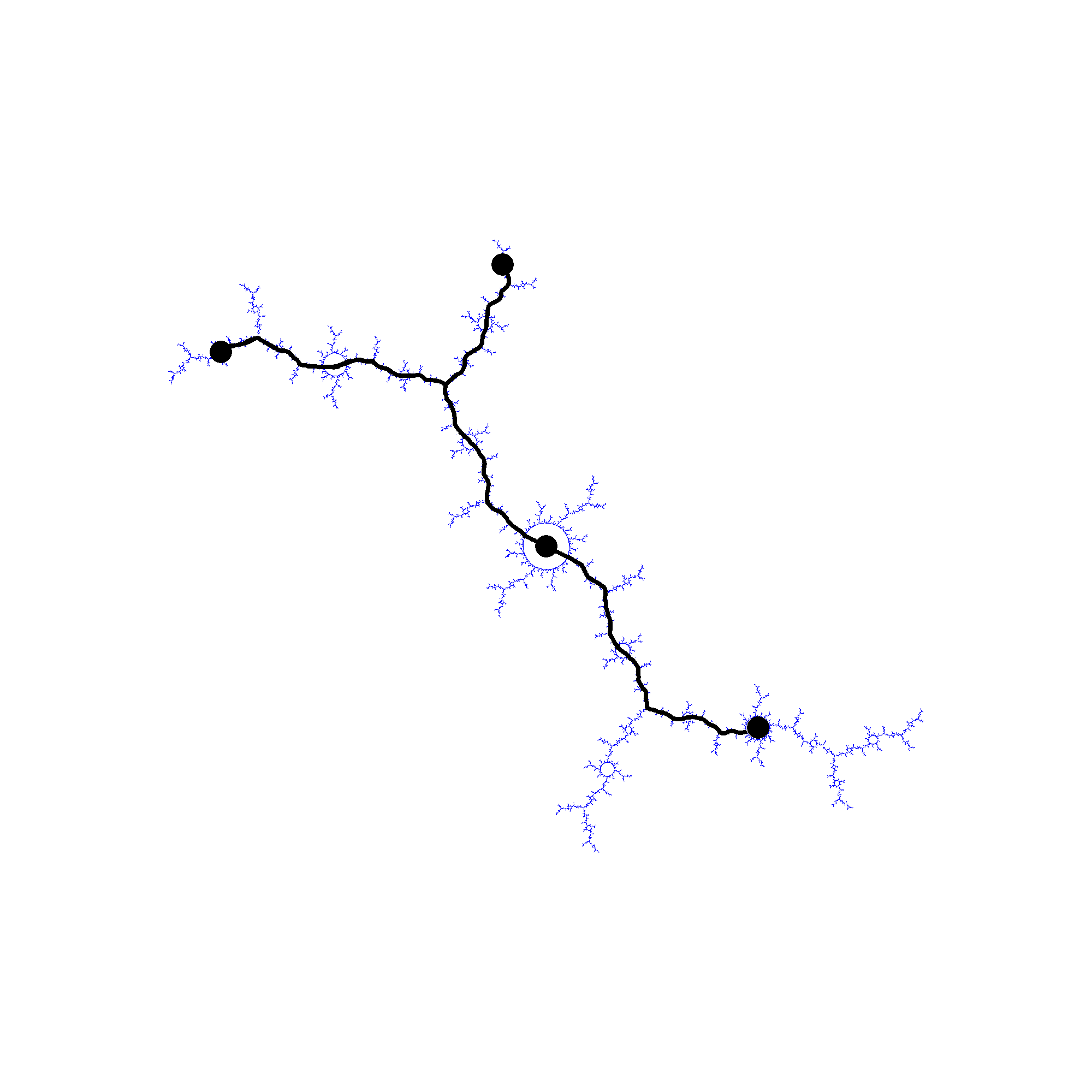
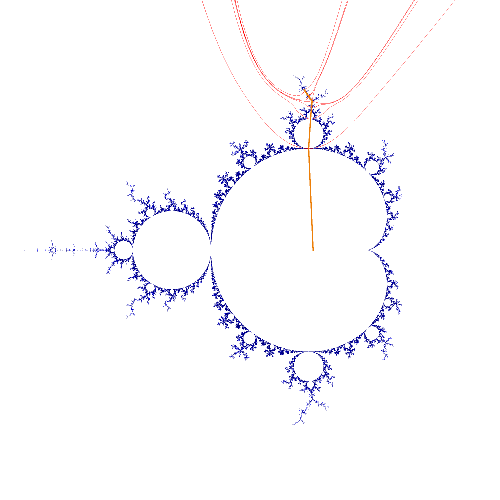
Figure 4. To the left: the Hubbard tree of the complex polynomial of period $4$ and characteristic angles $\theta=3/15,4/15$. To the right: the vein joining the center of the main cardioid with the main antenna in the $1/3$-limb ($\theta=1/4$), and external rays landing on it.

In parameter space, a generalization of the real slice is a vein: a vein $v$ is an embedded arc in $\mathcal{M}$, joining a parameter $c\in\partial\mathcal{M}$ with the center of the main cardioid. Given a vein $v$ and a parameter $c$ on $v$, we can define the set $P_{c}$ as the set of external angles of rays which land on $v$ closer than $c$ to the main cardioid:

$$P_{c}:=\{\theta\in\mathbb{R}/\mathbb{Z}\ :\ R_{M}(\theta)\textup{ lands on }v\cap[0,c]\}$$

where $[0,c]$ means the segment of vein joining $c$ to the center of the main cardioid (see Figure 4, right).

Note that the set of topologically finite parameters contain the postcritically finite ones but it is much larger: indeed, every parameter $c\in\partial\mathcal{M}$ which is biaccessible (i.e. it belongs to some vein) is topologically finite (see section 4).

In the $\frac{p}{q}$-limb, there is a unique parameter $c_{p/q}$ such that the critical point lands on the $\beta$ fixed point after $q$ iterates (i.e. $f^{q}(0)=\beta$). The vein $v_{p/q}$ joining $c_{p/q}$ to $c=0$ will be called the principal vein of angle $p/q$. Note that $v_{1/2}$ is the real axis, while $v_{1/3}$ is the vein constructed by Branner and Douady [BD]. We can now extend the result of Theorem 1.1 to principal veins:

Theorem 1.3.

Let $v=v_{p/q}$ be principal vein in the Mandelbrot set, and $c\in v\cap\partial\mathcal{M}$ a parameter along the vein. Then we have the equality

$$\frac{h_{top}(f_{c}\mid_{T_{c}})}{\log 2}=\textup{H.dim }H_{c}=\textup{H.dim }P_{c}.$$

We conjecture that the previous equality holds along any vein $v$. Note that the statement can be given in more symmetric terms in the following way. If one defines for each $A\subseteq\mathcal{M}$,

$$\Theta_{M}(A):=\{\theta\in S^{1}\ :\ R_{M}(\theta)\textup{ lands on }A\}$$

and similarly, for each $A\subseteq J(f_{c})$, the set

$$\Theta_{c}(A):=\{\theta\in S^{1}\ :\ R_{c}(\theta)\textup{ lands on }A\}$$

where $R_{c}(\theta)$ is the external ray at angle $\theta$ in the dynamical plane for $f_{c}$, then Theorem 1.3 is equivalent to the statement

$$\textup{H.dim }\Theta_{c}([0,c])=\textup{H.dim }\Theta_{M}([0,c]).$$

1.2. Pseudocenters and real hyperbolic windows

The techniques we use in the proof rely on the combinatorial analysis of the symbolic dynamics, and many ideas come from a connection with the dynamics of continued fractions. Indeed, on a combinatorial level the structure of the real slice of the Mandelbrot set is isomorphic to the structure of the bifurcation set $\mathcal{E}$ for continued fractions [BCIT], so we can use the combinatorial tools we developed in that case ([CT], [CT2]) to analyze the quadratic family.

For instance, in [CT], a key concept is the pseudocenter of an interval, namely the (unique!) rational number with the smallest denominator. When translated to the world of binary expansions, used to describe the parameter space of quadratic polynomials, the definition becomes

Definition 1.4.

The pseudocenter of a real interval $[a,b]$ with $|a-b|<1$ is the unique dyadic rational number with shortest binary expansion.

E.g., the pseudocenter of the interval $[\frac{13}{15},\frac{14}{15}]$ is $\frac{7}{8}=0.111$, since $\frac{13}{15}=0.\overline{1101}$ and $\frac{14}{15}=0.\overline{1110}$. Recall that a hyperbolic component $W\subseteq\mathcal{M}$ is a connected, open subset of parameters $c$ for which the critical point of $f_{c}$ is attracted to a periodic cycle. If $W$ intersects the real axis, we define the hyperbolic window associated to $W$ to be the interval $(\theta_{2},\theta_{1})\subseteq[0,1/2]$, where the rays $R_{M}(\theta_{1})$ and $R_{M}(\theta_{2})$ land on $\partial W\cap\mathbb{R}$.

By translating the bisection algorithm of ([CT], section 2.4) in terms of kneading sequences, we get the following algorithm to generate all real hyperbolic windows (see section 9.3).

Theorem 1.5.

The set of all real hyperbolic windows in the Mandelbrot set can be generated as follows. Let $c_{1}<c_{2}$ be two real parameters on the boundary of $\mathcal{M}$, with external angles $0\leq\theta_{2}<\theta_{1}\leq\frac{1}{2}$. Let $\theta^{*}$ be the dyadic pseudocenter of the interval $(\theta_{2},\theta_{1})$, and let

$$\theta^{*}=0.s_{1}s_{2}\dots s_{n-1}s_{n}$$

be its binary expansion, with $s_{n}=1$. Then the hyperbolic window of smallest period in the interval $(\theta_{2},\theta_{1})$ is the interval of external angles $(\alpha_{2},\alpha_{1})$ with

$$\begin{array}[]{ccc}\alpha_{2}&:=&0.\overline{s_{1}s_{2}\dots s_{n-1}}\\ \alpha_{1}&:=&0.\overline{s_{1}s_{2}\dots s_{n-1}\check{s}_{1}\check{s}_{2}\dots\check{s}_{n-1}}\end{array}$$

where $\check{s_{i}}:=1-s_{i}$. All real hyperbolic windows are obtained by iteration of this algorithm, starting with $\theta_{2}=0$, $\theta_{1}=1/2$.

1.3. Thurston’s point of view

The results of this paper relate to recent work of W. Thurston, who looked at the entropy of Hubbard trees as a function of the external angle. Indeed, every external angle $\theta$ of the Mandelbrot set combinatorially determines a lamination (see section 3) and the lamination determines an abstract Hubbard tree, of which we can compute the entropy $h(\theta)$.

Thurston produced very interesting pictures (Figure 5), suggesting that the complexity of the Mandelbrot set is encoded in the combinatorics of the Hubbard tree, and the variation in entropy reflects the geometry of $\mathcal{M}$.

In this sense, Theorems 1.1 and 1.3 contribute to this program: in fact, the entropy grows as one goes further from the center of $\mathcal{M}$ (see also [TaoL]), and our results make precise the relationship between the increase in entropy and the increased hairiness of the Mandelbrot set.

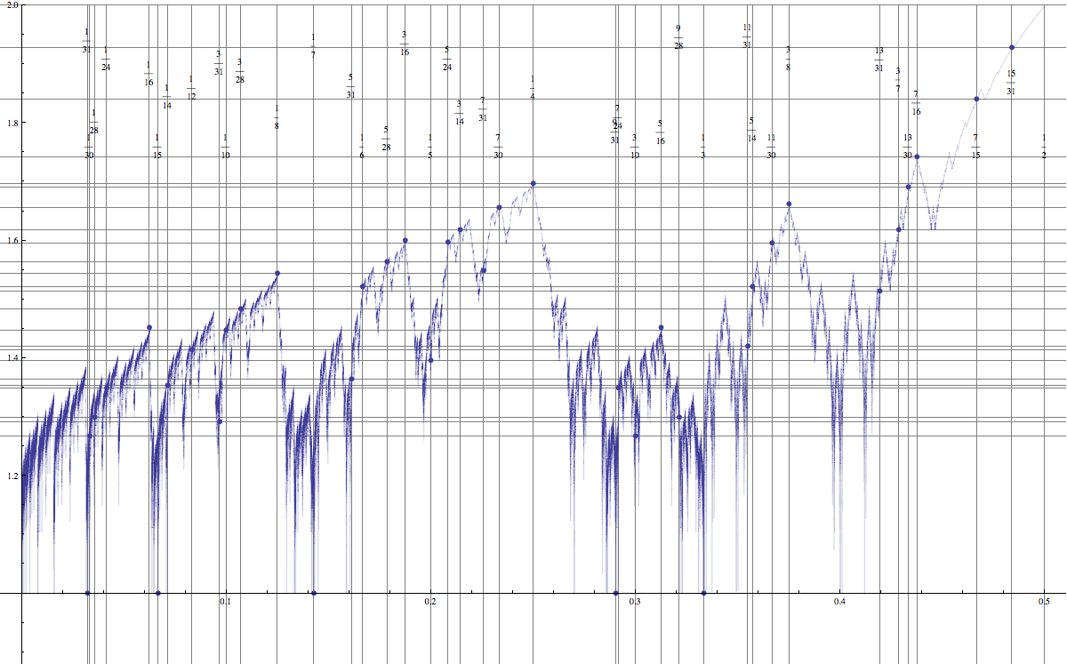
Figure 5. Entropy of Hubbard trees as a function of the external angle (by W. Thurston).

Bruin and Schleicher [BS] recently proved that entropy is continuous as a function of the external angle.

Note that Thurston’s approach is in some sense dual to ours, since we look at the variation of entropy along the veins, i.e. from “inside” the Mandelbrot set as opposed to from “outside” as a function of the external angle.

We point out that the idea of the pseudocenter described in the introduction seems also to be fruitful to study the entropy of the Hubbard tree as a function of the external angle: indeed, we conjecture that the maximum of the entropy on any wake is achieved precisely at its pseudocenter. Let us denote by $h(\theta)$ the entropy of the Hubbard tree corresponding to the parameter of external angle $\theta$.

Conjecture 1.6.

Let $\theta_{1}<\theta_{2}$ be two external angles whose rays $R_{M}(\theta_{1})$, $R_{M}(\theta_{2})$ land on the same parameter in the boundary of the Mandelbrot set. Then the maximum of entropy on the interval $[\theta_{1},\theta_{2}]$ is attained at its pseudocenter:

$$\max_{\theta\in[\theta_{1},\theta_{2}]}h(\theta)=h(\theta^{*})$$

where $\theta^{*}$ is the pseudocenter of the interval $[\theta_{1},\theta_{2}]$.

1.4. Sketch of the argument

The proof of Theorem 1.1 is carried out in two steps. We first prove (Theorem 7.1 in section 7) the relationship between topological entropy $h_{top}(f_{c}\mid_{T_{c}})$ of the map restricted to the Hubbard tree and the Hausdorff dimension of the set $H_{c}$ of angles landing on the tree, for all topologically finite polynomials $f_{c}$. The bulk of the argument is then proving the identity of Hausdorff dimensions between the real Julia set and the slices of $\mathcal{M}$:

Theorem 1.7.

For any $c\in[-2,\frac{1}{4}]$, we have the equality

$$\textup{H.dim }S_{c}=\textup{H.dim }P_{c}.$$

It is not hard to show that $P_{c}\subseteq H_{c}\subseteq S_{c}$ for any real parameter $c$ (Corollary 8.7); it is much harder to give a lower bound for the dimension of $P_{c}$ in terms of the dimension of $H_{c}$; indeed, it seems impossible to include a copy of $H_{c}$ in $P_{c}$ when $c$ belongs to some tuning window, i.e. to some baby Mandelbrot set. However, for non-renormalizable parameters we can prove the following:

Proposition 1.8.

Given a non-renormalizable, real parameter $c$ and another real parameter $c^{\prime}>c$, there exists a piecewise linear map $F:\mathbb{R}/\mathbb{Z}\to\mathbb{R}/\mathbb{Z}$ such that

$$F(H_{c^{\prime}})\subseteq P_{c}.$$

The proposition implies equality of dimension for all non-renormalizable parameters. By applying tuning operators, we then get equality for all finitely-renormalizable parameters, which are dense hence the result follows from continuity.

Proposition 1.8 will be proved in section 10. Its proof relies on the definition of a class of parameters, which we call dominant, which are a subset of the set of non-renormalizable parameters. We will show that for these parameters (which can be defined purely combinatorially) it is easier to construct an inclusion of the Hubbard tree into parameter space; finally, the most technical part (section 11.3) will be proving that such parameters are dense in the set of non-renormalizable angles.

In order to establish the result for complex veins, we first prove continuity of entropy along veins by a version of kneading theory for Hubbard trees (section 13). Finally, we transfer the inclusion of Proposition 1.8 from the real vein to the other principal vein via a combinatorial version of the Branner-Douady surgery (section 14).

1.5. Remarks and acknowledgements

The history of this paper is quite interesting. After the discovery of the connection between continued fractions and the real slice of $\mathcal{M}$ [BCIT], the statement for the real case (Theorem 1.1) came out of discussions with Carlo Carminati in spring 2011, as an application of our combinatorial techniques (indeed, modulo translation to the complex dynamics language, the essential arguments are contained in [CT2]). At about the same time, I have been informed of the recent work of W. Thurston on the entropy of Hubbard trees, which sparked new interest and inspired the generalization to complex veins.

I especially wish to thank A.M. Benini, Tan Lei, and C.T. McMullen for useful conversations, and D. Schleicher for pointing out reference [Ri]. Some of the pictures have been created with the software mandel of W. Jung.

2. External rays

Let $f(z)$ be a monic polynomial of degree $d$. Recall that the filled Julia set $K(f)$ is the set of points which do not escape to infinity under iteration:

$$K(f):=\{z\in\mathbb{C}\ :\ f^{n}(z)\textup{ does not tend to }\infty\textup{ as }n\to\infty\}.$$

The Julia set $J(f)$ is the boundary of $K(f)$. If $K(f)$ is connected, then the complement of $K(f)$ in the Riemann sphere is simply connected, so it can be uniformized by the Riemann mapping $\Phi:\hat{\mathbb{C}}\setminus\overline{\mathbb{D}}\to\hat{\mathbb{C}}\setminus K(f)$ which maps the exterior of the closed unit disk $\overline{\mathbb{D}}$ to the exterior of $K(f)$. The Riemann mapping is unique once we impose $\Phi(\infty)=\infty$ and $\Phi^{\prime}(\infty)=1$. With this choice, $\Phi$ conjugates the action of $f$ on the exterior of the filled Julia set to the map $z\mapsto z^{d}$, i.e.

(1) $$f(\Phi(z))=\Phi(z^{d}).$$

By Carathéodory’s theorem (see e.g. [Po]), the Riemann mapping extends to a continuous map $\overline{\Phi}$ on the boundary $\overline{\Phi}:\hat{\mathbb{C}}\setminus\mathbb{D}\to\hat{\mathbb{C}}\setminus\textup{int }K(f)$ if and only if the Julia set is locally connected. If this is the case, the restriction of $\overline{\Phi}$ to the boundary is sometimes called the Carathéodory loop and it will be denoted as

$$\gamma:\mathbb{R}/\mathbb{Z}\to J(f).$$

As a consequence of the eq. (1), the action of $f$ on the set of angles is semiconjugate to multiplication by $d$ (mod $1$):

(2) $$\gamma(d\cdot\theta)=f(\gamma(\theta))\qquad\textup{for each }\theta\in\mathbb{R}/\mathbb{Z}.$$

In the following we will only deal with the case of quadratic polynomials of the form $f_{c}(z):=z^{2}+c$, so $d=2$ and we will denote as

$$D(\theta):=2\cdot\theta\mod 1$$

the doubling map of the circle. Moreover, we will add the subscript $c$ when we need to make the dependence on the polynomial $f_{c}$ more explicit. Given $\theta\in\mathbb{R}/\mathbb{Z}$, the external ray $R_{c}(\theta)$ is the image of the radial arc at angle $2\pi\theta$ via the Riemann mapping $\Phi_{c}:\hat{\mathbb{C}}\setminus\overline{\mathbb{D}}\to\hat{\mathbb{C}}\setminus K(f_{c})$:

$$R_{c}(\theta):=\{\Phi_{c}(\rho e^{2\pi i\theta})\}_{\rho>1}.$$

The ray $R_{c}(\theta)$ is said to land at $x$ if

$$\lim_{\rho\to 1^{+}}\Phi_{c}(\rho e^{2\pi i\theta})=x.$$

If the Julia set is locally connected, then all rays land; in general, by Fatou’s theorem, the set of angles for which $R_{c}(\theta)$ does not land has zero Lebesgue measure, and indeed it also has zero capacity and hence zero Hausdorff dimension (see e.g. [Po]). It is however known that there exist non-locally connected Julia sets for polynomials [Mi2]. The ray $R_{c}(0)$ always lands on a fixed point of $f_{c}$ which is traditionally called the $\beta$ fixed point and denoted as $\beta$. The other fixed point of $f_{c}$ is called the $\alpha$ fixed point. Note that in the case $c=\frac{1}{4}$ one has $\alpha=\beta$. Finally, the critical point of $f_{c}$ will be denoted by $0$, and the critical value by $c$.

Analogously to the Julia sets, the exterior of the Mandelbrot set can be uniformized by the Riemann mapping

$$\Phi_{M}:\hat{\mathbb{C}}\setminus\overline{\mathbb{D}}\rightarrow\hat{\mathbb{C}}\setminus\mathcal{M}$$

with $\Phi_{M}(\infty)=\infty$, and $\Phi^{\prime}(\infty)=1$, and images of radial arcs are called external rays. Every angle $\theta\in\mathbb{R}/\mathbb{Z}$ determines an external ray

$$R_{M}(\theta):=\Phi_{M}(\{\rho e^{2\pi i\theta}:\rho>1\})$$

which is said to land at $x$ if the limit $\lim_{\rho\to 1^{+}}\Phi_{M}(\rho e^{2\pi i\theta})$ exists. According to the MLC conjecture [DH], the Mandelbrot set is locally connected, and therefore all rays land on some point of the boundary of $\mathcal{M}$.

2.1. Biaccessibility and regulated arcs

A point $z\in J(f_{c})$ is called accessible if it is the landing point of at least one external ray. It is called biaccessible if it is the landing point of at least two rays, i.e. there exist $\theta_{1},\theta_{2}$ two distinct angles such that $R_{c}(\theta_{1})$ and $R_{c}(\theta_{2})$ both land at $z$. This is equivalent to say that $J(f_{c})\setminus\{z\}$ is disconnected.

Let $K=K(f_{c})$ be the filled Julia set of $f_{c}$. Assume $K$ is connected and locally connected. Then it is also path-connected (see e.g. [Wi], Chapter 8), so given any two points $x,y$ in $K$, there exists an arc in $K$ with endpoints $x,y$.

If $K$ has no interior, then the arc is uniquely determined by its endpoints $x$, $y$. Let us now describe how to choose a canonical representative inside the Fatou components in the case $K$ has interior. In this case, each bounded Fatou component eventually maps to a periodic Fatou component, which either contains an attracting cycle, or it contains a parabolic cycle on its boundary, or it is a periodic Siegel disk.

Since we will not deal with the Siegel disk case in the rest of the paper, let us assume we are in one of the first two cases. Then there exists a Fatou component $U_{0}$ which contains the critical point, and a biholomorphism $\phi_{0}:U_{0}\to\mathbb{D}$ to the unit disk mapping the critical point to $0$. The preimages $\phi_{0}^{-1}(\{\rho e^{2\pi i\theta}\ :\ 0\leq\rho<1\})$ of radial arcs in the unit disk are called radial arcs in $U_{0}$. Any other bounded Fatou component $U$ is eventually mapped to $U_{0}$; let $k\geq 0$ be the smallest integer such that $f_{c}^{k}(U)=U_{0}$. Then the map $\phi:=\phi_{0}\circ f_{c}^{k}$ is a biholomorphism of $U$ onto the unit disk, and we define radial arcs to be preimages under $\phi$ of radial arcs in the unit disk.

An embedded arc $I$ in $K$ is called regulated (or legal in Douady’s terminology [Do2]) if the intersection between $I$ and the closure of any bounded Fatou component is contained in the union of at most two radial arcs. With this choice, given any two points $x,y$ in $K$, there exists a unique regulated arc in $K$ with endpoints $x,y$ ([Za1], Lemma 1). Such an arc will be denoted by $[x,y]$, and the corresponding open arc by $(x,y):=[x,y]\setminus\{x,y\}$. A regulated tree inside $K$ is a finite tree whose edges are regulated arcs. Note that, in the case $K$ has non-empty interior, regulated trees as defined need not be invariant for the dynamics, because $f_{c}$ need not map radial arcs to radial arcs. However, by construction, radial arcs in any bounded Fatou component $U$ different from $U_{0}$ map to radial arcs in $f_{c}(U)$. In order to deal with $U_{0}$, we need one further hypothesis. Namely, we will assume that $f_{c}$ has an attracting or parabolic cycle of period $p$ with real multiplier. Then we can find a parametrization $\phi_{0}:U_{0}\to\mathbb{D}$ such that the interval $I:=\phi_{0}^{-1}((-1,1))$ is preserved by the $p$-th iterate of $f_{c}$, i.e. $f_{c}^{p}(I)\subseteq I$. The interval $I$ will be called the bisector of $U_{0}$. Now note that, if the regulated arc $[x,y]$ does not contain $0$ in its interior and it only intersects the critical Fatou component $U_{0}$ in its bisector, then we have

$$f_{c}([x,y])=[f_{c}(x),f_{c}(y)].$$

The spine of $f_{c}$ is the regulated arc $[-\beta,\beta]$ joining the $\beta$ fixed point to its preimage $-\beta$. The biaccessible points are related to the points which lie on the spine by the following lemma.

Lemma 2.1.

Let $f_{c}(z)=z^{2}+c$ be a quadratic polynomial whose Julia set is connected and locally connected. Then the set of biaccessible points is

$$\mathcal{B}=J(f_{c})\cap\bigcup_{n\geq 0}f_{c}^{-n}((-\beta,\beta)).$$

Proof.

Let $f=f_{c}$, and $x\in J(f)\cap(-\beta,\beta)$. The set $V:=R_{c}(0)\cup[-\beta,\beta]\cup R_{c}(1/2)$ disconnects the plane in two parts, $\mathbb{C}\setminus V=A_{1}\cup A_{2}$. We claim that $x$ is the limit of points in the basin of infinity $U_{\infty}$ on both sides of $V$, i.e. for each $i=1,2$ there exists a sequence $\{x_{n}\}_{n\in\mathbb{N}}\subseteq A_{i}\cap U_{\infty}$ with $x_{n}\to x$; since the Riemann mapping $\Phi$ extends continuously to the boundary, this is enough to prove that there exist two external angles $\theta_{1}\in(0,1/2)$ and $\theta_{2}\in(1/2,1)$ such that $R_{c}(\theta_{1})$ and $R_{c}(\theta_{2})$ both land on $x$. Let us now prove the claim; if it is not true, then there exists an open neighborhood $\Omega$ of $x$ and an index $i\in\{1,2\}$ such that $\Omega\cap A_{i}$ is connected and contained in the interior of the filled Julia set $K(f)$, hence $\Omega\cap A_{i}$ is contained in some bounded Fatou component. This implies that $\Omega\cap V$ lies in the closure of a bounded Fatou component, and $x$ on its boundary. However, this contradicts the definition of regulated arc, because if $U$ is a bounded Fatou component intersecting a regulated arc $I$, then $\partial U\cap I$ does not disconnect $\overline{U}\cap I$. Suppose now that $x\in J(f)$ is such that $f^{n}(x)$ belongs to $(-\beta,\beta)$ for some $n$. Then by the previous argument $f^{n}(x)$ is biaccessible, and since $f$ is a local homeomorphism outside the spine, $x$ is also biaccessible.

Conversely, suppose $x$ is biaccessible, and the two rays at angles $\theta_{1}$ and $\theta_{2}$ land on $x$, with $0<\theta_{1}<\theta_{2}<1$. Then there exists some $n$ for which $1/2\leq D^{n}(\theta_{2})-D^{n}(\theta_{1})<1$, hence $R_{c}(D^{n}(\theta_{1}))$ and $R_{c}(D^{n}(\theta_{2}))$ must lie on opposite sides with respect to the spine, and since they both land on $f^{n}(x)$, then $f^{n}(x)$ belongs to the spine. Since the point $\beta$ is not biaccessible ([Mc], Theorem 6.10), $f^{n}(x)$ must belong to $(-\beta,\beta)$. ∎

Lemma 2.2.

We have that $\alpha\in[0,c]$.

Proof.

Indeed, since $\alpha\in(-\beta,0)$ ([Za1], Lemma 5), we have $-\alpha\in(\beta,0)$ and $\alpha=f(-\alpha)\in(\beta,c)$. Thus, since $0\in(\alpha,\beta)$ we have $\alpha\in(0,c)$. ∎

Lemma 2.3.

For $x\in[0,\beta)$, we have $x\in(f(x),\beta)$.

Proof.

Let us consider the set $S=\{x\in[0,\beta]\ :\ x\in(\beta,f(x))\}$. The set is open by continuity of $f$. Since the $\beta$ fixed point is repelling, the set $S$ contains points in a neighborhood of $\beta$, so it is not empty. Suppose $S\neq[0,\beta)$ and let $x\in\partial S$, $x\neq\beta$. By continuity of $f$, $x$ must be a fixed point of $f$, but the only fixed point of $f$ in the arc is $\beta$. ∎

For more general properties of biaccessibility we refer to [Za1].

3. Laminations

A powerful tool to construct topological models of Julia sets and the Mandelbrot set is given by laminations, following Thurston’s approach. As we will see, laminations represent equivalence relations on the boundary of the disk arising from external rays which land on the same point. We now give the basic definitions, and refer to [Th1] for further details.

A geodesic lamination $\lambda$ is a set of hyperbolic geodesics in the closed unit disk $\overline{\mathbb{D}}$, called the leaves of $\lambda$, such that no two leaves intersect in $\mathbb{D}$, and the union of all leaves is closed.

A gap of a lamination $\lambda$ is the closure of a component of the complement of the union of all leaves. In order to represent Julia sets of quadratic polynomials, we need to restrict ourselves to invariant laminations.

Let $d\geq 2$. The map $g(z):=z^{d}$ acts on the boundary of the unit disk, hence it induces a dynamics on the set of leaves. Namely, the image of a leaf $\overline{pq}$ is defined as the leaf joining the images of the endpoint: $g(\overline{pq})=\overline{g(p)g(q)}$. A lamination $\lambda$ is forward invariant if the image of any leaf $L$ of $\lambda$ still belongs to $\lambda$. Note that the image leaf may be degenerate, i.e. consist of a single point on the boundary of the disk.

A lamination is invariant if in addition to being forward invariant it satisfies the additional conditions:

• Backward invariance: if $\overline{pq}$ is in $\lambda$, then there exists a collection of $d$ disjoint leaves in $\lambda$, each joining a preimage of $p$ to a preimage of $q$.

• Gap invariance: for any gap $G$, the hyperbolic convex hull of the image of $G_{0}=\overline{G}\cap S^{1}$ is either a gap, a leaf, or a single point.

In this paper we will only deal with quadratic polynomials, so $d=2$ and the invariant laminations for the map $g(z)=z^{2}$ will be called invariant quadratic laminations. A leaf of maximal length in a lamination is called a major leaf, and its image a minor leaf. Typically, a quadratic invariant lamination has $2$ major leaves, but the minor leaf is always unique.

If $J(f_{c})$ is a Julia set of a quadratic polynomial, one can define the equivalence relation $\sim_{c}$ on the unit circle $\partial\mathbb{D}$ by saying that $\theta_{1}\sim_{c}\theta_{2}$ if the rays $R_{c}(\theta_{1})$ and $R_{c}(\theta_{2})$ land on the same point.

From the equivalence relation $\sim_{c}$ one can construct a quadratic invariant lamination in the following way. Let $E$ be an equivalence class for $\sim_{c}$. If $E=\{\theta_{1},\theta_{2}\}$ contains two elements, then we define the leaf $L_{E}$ as $L_{E}:=(\theta_{1},\theta_{2})$. If $E=\{\theta\}$ is a singleton, then we define $L_{E}$ to be the degenerate leaf $L_{E}:=\{\theta\}$. Finally, if $E=\{\theta_{1},\dots,\theta_{k}\}$ contains more than two elements, with $0\leq\theta_{1}<\theta_{2}<\dots<\theta_{k}<1$, then we define $L_{E}$ to be the union of the leaves $L_{E}:=(\theta_{1},\theta_{2})\cup(\theta_{2},\theta_{3})\cup\dots\cup(\theta_{k},\theta_{1})$. Finally, we let the associated lamination $\lambda_{c}$ be

$$\lambda_{c}:=\bigcup_{E\textup{ equiv. class of }\sim_{c}}L_{E}.$$

The lamination $\lambda_{c}$ is an invariant quadratic lamination. The equivalence relation $\sim_{c}$ can be extended to a relation $\cong_{c}$ on the closed disk $\overline{\mathbb{D}}$ by taking convex hulls, and the quotient of the disk by $\cong_{c}$ is a model for the Julia set:

Theorem 3.1 ([Do2]).

If the Julia set $J(f_{c})$ is connected and locally connected, then it is homeomorphic to the quotient of $\overline{\mathbb{D}}$ by the equivalence relation $\cong_{c}$.

We define the the characteristic leaf of a quadratic polynomial $f_{c}$ with Julia set connected and locally connected to be the minor leaf of the invariant lamination $\lambda_{c}$. The endpoints of the characteristic leaf are called characteristic angles.

3.1. The abstract Mandelbrot set

In order to construct a model for the Mandelbrot set, Thurston [Th1] defined the quadratic minor lamination $QML$ as the union of the minor leaves of all quadratic invariant laminations (see Figure 6).

Figure 6. Thurston’s quadratic minor lamination. The quotient of the unit disk by the equivalence relation given by the lamination is a topological model for $\mathcal{M}$. Leaves which are symmetric with respect to complex conjugation (displayed thicker) correspond to rays landing on the real axis.

As in the Julia set case, the lamination determines an equivalence relation $\cong_{M}$ on $\overline{\mathbb{D}}$ by identifying points on the same leaf, and also points in the interior of finite ideal polygons whose sides are leaves. The quotient

$$\mathcal{M}_{abs}:=\overline{\mathbb{D}}/\cong_{M}$$

is called abstract Mandelbrot set. It is a compact, connected and locally connected space. Douady [Do2] constructed a continuous surjection

$$\pi_{M}:\mathcal{M}\to\mathcal{M}_{abs}$$

which is injective if and only if $\mathcal{M}$ is locally connected.

The idea behind the construction is that leaves of $QML$ connect external angles whose corresponding rays in parameter space land on the same point. However, since we do not know whether $\mathcal{M}$ is locally connected, additional care is required. Indeed, let $\sim_{M}$ denote the equivalence relation on $\partial\mathbb{D}$ induced by the lamination $QML$, and $\theta_{1}\asymp_{M}\theta_{2}$ denote that the external rays $R_{M}(\theta_{1})$ and $R_{M}(\theta_{2})$ land on the same point. The following theorem summarizes a few key results comparing the analytic and combinatorial models of the Mandelbrot set:

Theorem 3.2.

Let $\theta_{1},\theta_{2}\in\mathbb{R}/\mathbb{Z}$ be two angles. Then the following are true:

1. if $\theta_{1}\asymp_{M}\theta_{2}$, then $\theta_{1}\sim_{M}\theta_{2}$;

2. if $\theta_{1}\sim_{M}\theta_{2}$ and $\theta_{1},\theta_{2}$ are rational, then $\theta_{1}\asymp_{M}\theta_{2}$;

3. if $\theta_{1}\sim_{M}\theta_{2}$ and $\theta_{1},\theta_{2}$ are not infinitely renormalizable, then $\theta_{1}\asymp_{M}\theta_{2}$.

Proof.

(1) and (2) are contained in ([Th1], Theorem A.3). (3) follows from Yoccoz’s theorem on landing of rays at finitely renormalizable parameters (see [Hu] for the proof). Indeed, Yoccoz proves that external rays $R_{M}(\theta)$ with non-infinitely renormalizable combinatorics land, and moreover that the intersections of nested parapuzzle pieces contain a single point. Along the boundary of each puzzle piece lie pairs of external rays with rational angles (see also [Hu], sections 5 and 12) which land on the same point, and since the intersection of the nested sequence of puzzle pieces is a single point $c\in\partial\mathcal{M}$, the rays $\theta_{1}$ and $\theta_{2}$ land on the same point $c$. ∎

The following criterion makes it possible to check whether a leaf belongs to the quadratic minor lamination by looking at its dynamics under the doubling map:

Proposition 3.3 ([Th1]).

A leaf $m$ is the minor leaf of some invariant quadratic lamination (i.e. it belongs to $QML$) if and only if the following three conditions are met:

• all forward images of $m$ have disjoint interiors;

• the length of any forward image of $m$ is never less than the length of $m$;

• if $m$ is a non-degenerate leaf, then $m$ and all leaves on the forward orbit of $m$ are disjoint from the interiors of the two preimage leaves of $m$ of length at least $1/3$.

For the rest of the paper we shall work with the abstract, locally connected model of $\mathcal{M}$ and study its dimension using combinatorial techniques; only at the very end (Proposition 14.13) we shall compare the analytical and combinatorial models and prove that our results hold for the actual Mandelbrot set even without assuming the MLC conjecture.

4. Hubbard trees

Assume now that the polynomial $f=f_{c}(z)=z^{2}+c$ has connected Julia set (i.e. $c\in\mathcal{M}$), and no attracting fixed point (i.e. $c$ lies outside the main cardioid). The critical orbit of $f$ is the set $Crit(f):=\{f^{k}(0)\}_{k\geq 0}$. Let us now give the fundamental

Definition 4.1.

The Hubbard tree $T$ for $f$ is the smallest regulated tree which contains the critical orbit, i.e.

$$T:=\bigcup_{i,j\geq 0}[f^{i}(0),f^{j}(0)].$$

Note that, according to this definition, the set $T$ need not be closed in general. We shall establish a few fundamental properties of Hubbard trees.

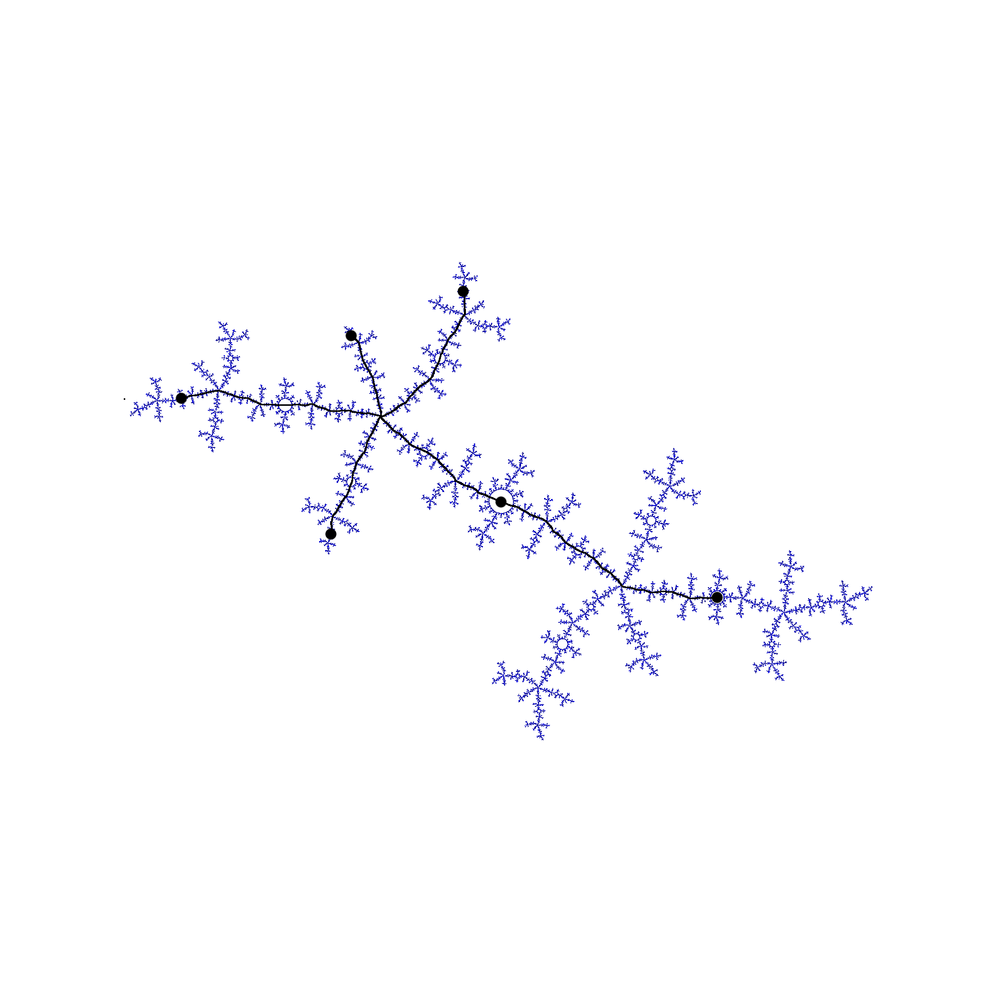
Figure 7. The Hubbard tree of the quadratic polynomial with characteristic leaf $(19/63,20/63)$. The map $f_{c}$ is postcritically finite, and the critical point belongs to a cycle of period $6$. The parameter $c$ belongs to the principal vein in the $2/5$-limb.

Lemma 4.2.

The following properties hold:

1. $T$ is the smallest forward-invariant set which contains the regulated arc $[\alpha,0]$;

2. $T=\bigcup_{n\geq 0}[\alpha,f^{n}(0)]$.

Proof.

Let now $T_{1}$ be the smallest forward-invariant set which contains the regulated arc $[\alpha,0]$. By definition, $T$ is forward-invariant and contains $[\alpha,0]$ since $\alpha\in[0,c]$, so $T_{1}\subseteq T$. Let now

$$T_{2}:=\bigcup_{n\geq 0}[\alpha,f^{n}(0)].$$

Since $[f^{i}(0),f^{j}(0)]\subseteq[\alpha,f^{i}(0)]\cup[\alpha,f^{j}(0)]$, then $T\subseteq T_{2}$. By definition,

$$T_{1}=\bigcup_{n\geq 0}f^{n}([\alpha,0]).$$

Since $f^{i}([\alpha,0])\supseteq[\alpha,f^{i}(0)]$, then $T_{2}\subseteq T_{1}$, hence $T=T_{1}=T_{2}$. ∎

The tree thus defined need not have finitely many edges. However, in the following we will restrict ourself to the case when $T$ is a finite tree. Let us introduce the definition:

Definition 4.3.

A polynomial $f$ is topologically finite if the Julia set is locally connected and the Hubbard tree $T$ is homeomorphic to a tree with finitely many edges.

Recall that a polynomial is called postcritically finite if the critical orbit is finite. Postcritically finite polynomials are also topologically finite, but it turns out that the class of topologically finite polynomials is much bigger and indeed it contains all polynomials along the veins of the Mandelbrot set (see also section 12.1).

Proposition 4.4.

Let $f$ have locally connected Julia set. Suppose there is an integer $n\geq 1$ such that $f^{n}(0)$ lies on the regulated arc $[\alpha,\beta]$, and let $N$ be the smallest such integer. Then $f$ is topologically finite, and the Hubbard tree $T$ of $f$ is given by

$$T=\bigcup_{i=0}^{N}[\alpha,f^{i}(0)].$$

Proof.

Let $T_{N}:=\bigcup_{i=0}^{N}[\alpha,f^{i}(0)]$. By Lemma 4.2 (2), $T_{N}\subseteq T$. Note now that for each $i$ we have

$$f([\alpha,f^{i}(0)])\subseteq[\alpha,c]\cup[\alpha,f^{i+1}(0)]$$

thus

$$f(T_{N})\subseteq T_{N}\cup[\alpha,f^{N+1}(0)].$$

Now, either $f^{N}(0)$ lies in $[\alpha,-\alpha]$, or by Lemma 2.3, $f^{N}(0)$ lies between $\beta$ and $f^{N+1}(0)$. In the first case, $[\alpha,f^{N+1}(0)]\subseteq[\alpha,c]$ and in the second case $[\alpha,f^{N+1}(0)]\subseteq[\alpha,f^{N}(0)]$; in both cases, $[\alpha,f^{N+1}(0)]\subseteq T_{N}$, so $T_{N}$ is forward-invariant and it contains $[\alpha,0]$, so it contains $T$ by Lemma 4.2 (1). ∎

Proposition 4.5.

If the Julia set of $f$ is locally connected and the critical value $c$ is biaccessible, then $f$ is topologically finite.

Proof.

Since $c$ is biaccessible, by Lemma 2.1 there exists $n\geq 0$ such that $f^{n}(c)$ belongs to the spine $[-\beta,\beta]$ of the Julia set. Then either $f^{n}(c)$ or $f^{n+1}(c)$ lie on $[\alpha,\beta]$, so $f$ is topologically finite by Proposition 4.4. ∎

Let us define the extended Hubbard tree $\widetilde{T}$ to be the union of the Hubbard tree and the spine:

$$\widetilde{T}:=T\cup[-\beta,\beta].$$

Note the extended tree is also forward invariant, i.e. $f(\widetilde{T})\subseteq\widetilde{T}$. Moreover, it is related to the usual Hubbard tree in the following way:

Lemma 4.6.

The extended Hubbard tree eventually maps to the Hubbard tree:

$$\widetilde{T}\setminus\{\beta,-\beta\}\subseteq\bigcup_{n\geq 0}f^{-n}(T).$$

Proof.

Since $f([\alpha,-\beta))=[\alpha,\beta)$, we just need to check that every element $z\in[\alpha,\beta)$ eventually maps to the Hubbard tree. Indeed, either there exists $n\geq 0$ such that $f^{n}(z)\in[\alpha,c]\subseteq T$, or, by Lemma 2.3, the sequence $\{f^{n}(z)\}_{z\geq 0}$ all lies on $[0,\beta)$ and it is ordered along the segment, i.e. for each $n$, $f^{n+1}(z)$ lies in between $0$ and $f^{n}(z)$. Then the sequence must have a limit point, and such limit point would be a fixed point of $f$. However, $f$ has no fixed points on $[0,\beta)$, contradiction. ∎

4.1. Valence

If $T$ is a finite tree, then the degree of a point $x\in T$ is the number of connected components of $T\setminus\{x\}$, and is denoted by $deg(x)$. Moreover, let us denote by $deg(T)$ denote the largest degree of a point on the tree:

$$deg(T):=\max\{deg(x)\ :\ x\in T\}.$$

On the other hand, for each $z\in J(f)$, we call valence of $z$ the number of external rays which land on $z$ and denote it as

$$val(z):=\#\{\theta\in\mathbb{R}/\mathbb{Z}\ :\ R_{c}(\theta)\textup{ lands on }z\}.$$

The valence of $z$ also equals the number of connected components of $J(f)\setminus\{z\}$ ([Mc], Theorem 6.6), also known as the Urysohn-Menger index of $J(f)$ at $z$.

Proposition 4.7.

Let $T$ be the extended Hubbard tree for a topologically finite quadratic polynomial $f$. Then the number of rays $N$ landing on $x\in T$ is bounded above by

$$N\leq 2\cdot deg(T).$$

The proposition follows easily from the

Lemma 4.8.

Let $T$ be the extended Hubbard tree for $f$, and $x\in T$ a point on the tree which never maps to the critical point. Then the number of rays $N$ landing on $x$ is bounded above by

$$N\leq\max\{deg(f^{n}(x))\ :\ n\geq 0\}.$$

Proof.

Note that, since the forward orbit of $x$ does not contain the critical point, $f^{n}$ is a local homeomorphism in a neighborhood of $x$; thus, for each $n\geq 0$, $val(f^{n}(x))=val(x)$ and $deg(f^{n}(x))\geq deg(x)$. Suppose now the claim is false: let $N$ be such that $deg(f^{N}(x))=\max\{deg(f^{n}(x))\ :\ n\geq 0\}<val(x)$, and denote $y=f^{N}(x)$. Then there are two angles $\theta_{1}$, $\theta_{2}$ such that the rays $R_{c}(\theta_{1})$ and $R_{c}(\theta_{2})$ both land at $y$, and the sector between $R_{c}(\theta_{1})$ and $R_{c}(\theta_{2})$ does not intersect the tree. Then, there exists $M\geq 0$ such that the rays $R_{c}(D^{M}(\theta_{1}))$ and $R_{c}(D^{M}(\theta_{2}))$ lie on opposite sides of the spine, thus their common landing point $z:=f^{M}(y)$ must lie on the spine. Moreover, since $val(z)=val(x)\geq 2$ while only one ray lands on the $\beta$ fixed point, $z$ must lie in the interior of the spine. This means that the sector between the rays $R_{c}(D^{M}(\theta_{1}))$ and $R_{c}(D^{M}(\theta_{2}))$ intersects the spine, so $deg(f^{M}(y))>deg(y)$, contradicting the maximality of $N$. ∎

Proof of Proposition 4.7.

If $val(x)>0$, then $x$ lies in the Julia set $J(f_{c})$. Now, if the forward orbit of $x$ does not contain the critical point, the claim follows immediately from the Lemma. Otherwise, let $n\geq 0$ be such that $f^{n}(x)=0$ is the critical point. Note that this $n$ is unique, because otherwise the critical point would be periodic, so it would not lie in the Julia set. Hence, by applying the Lemma to the critical value $f^{n+1}(x)$, we have

$$val(f^{n+1}(x))\leq deg(T).$$

Finally, since the map $f_{c}$ is locally a double cover at the critical point,

$$val(x)=val(f^{n}(x))=2\cdot val(f^{n+1}(x))\leq 2\cdot deg(T).$$

∎

5. Topological entropy

Let $f:X\to X$ be a continuous map of a compact metric space $(X,d)$. A measure of the complexity of the orbits of the map is given by its topological entropy. Let us now recall its definition. Useful references are [dMvS] and [CFS].

Given $x\in X$, $\epsilon>0$ and $n$ an integer, we define the ball $B_{f}(x,\epsilon,n)$ as the set of points whose orbit remains close to the orbit of $x$ for the first $n$ iterates:

$$B_{f}(x,\epsilon,n):=\{y\in X\ :\ d(f^{i}(x),f^{i}(y))<\epsilon\ \forall 0\leq i\leq n\}.$$

A set $E\subseteq X$ is called $(n,\epsilon)$-spanning if every point of $X$ remains close to some point of $E$ for the first $n$ iterates, i.e. if $X=\bigcup_{x\in E}B_{f}(x,\epsilon,n)$. Let $N(n,\epsilon)$ be the minimal cardinality of a $(n,\epsilon)$-spanning set. The topological entropy is the growth rate of $N(n,\epsilon)$ as a function of $n$:

Definition 5.1.

The topological entropy of the map $f:X\to X$ is defined as

$$h_{top}(f):=\lim_{\epsilon\to 0^{+}}\lim_{n\to\infty}\frac{1}{n}\log N(n,\epsilon).$$

When $f$ is a piecewise monotone map of a real interval, it is easier to compute the entropy by looking at the number of laps. Recall the lap number $L(g)$ of a piecewise monotone interval map $g:I\to I$ is the smallest cardinality of a partition of $I$ in intervals such that the restriction of $g$ to any such interval is monotone. The following result of Misiurewicz and Szlenk relates the topological entropy to the growth rate of the lap number of the iterates of $f$:

Theorem 5.2 ([MS]).

Let $f:I\to I$ be a piecewise monotone map of a close bounded interval $I$, and let $L(f^{n})$ be the lap number of the iterate $f^{n}$. Then the following equality holds:

$$h(f)=\lim_{n\to\infty}\frac{1}{n}\log L(f^{n}).$$

Another useful property of topological entropy is that it is invariant under dynamical extensions of bounded degree:

Proposition 5.3 ([Bo]).

Let $f:X\to X$ and $g:Y\to Y$ be two continuous maps of compact metric spaces, and let $\pi:X\to Y$ a continuous, surjective map such that $g\circ\pi=\pi\circ f$. Then

$$h_{top}(g)\leq h_{top}(f).$$

Moreover, if there exists a finite number $d$ such that for each $y\in Y$ the fiber $\pi^{-1}(y)$ has cardinality always smaller than $d$, then

$$h_{top}(g)=h_{top}(f).$$

In order to resolve the ambiguities arising from considering different restrictions of the same map, if $K$ is an $f$-invariant set we shall use the notation $h_{top}(f,K)$ to denote the topological entropy of the restriction of $f$ to $K$.

Proposition 5.4 ([Do3], Proposition 3).

Let $f:X\to X$ a continuous map of a compact metric space, and let $Y$ be a closed subset of $X$ such that $f(Y)\subseteq Y$. Suppose that, for each $x\in X$, the distance $d(f^{n}(x),Y)$ tends to zero, uniformly on any compact subset of $X\setminus Y$. Then $h_{top}(f,Y)=h_{top}(f,X)$.

The following proposition is the fundamental step to relate entropy and Hausdorff dimension of invariant subsets of the circle ([Fu], Proposition III.1; see also [Bi]):

Proposition 5.5.

Let $d\geq 1$, and $\Omega\subset\mathbb{R}/\mathbb{Z}$ be a closed, invariant set for the map $Q(x):=dx\mod 1$. Then the topological entropy of the restriction of $Q$ to $\Omega$ is related to the Hausdorff dimension of $\Omega$ in the following way:

$$\textup{H.dim }\Omega=\frac{h_{top}(Q,\Omega)}{\log d}.$$

6. Invariant sets of external angles

Let $f_{c}$ be a topologically finite quadratic polynomial, and $T_{c}$ its Hubbard tree. One of the main players in the rest of the paper is the set $H_{c}$ of angles of external rays landing on the Hubbard tree:

$$H_{c}:=\{\theta\in\mathbb{R}/\mathbb{Z}\ :R_{c}(\theta)\textup{ lands on }T_{c}\}.$$

Note that, since $T_{c}$ is compact and the Carathéodory loop is continuous by local connectivity, $H_{c}$ is a closed subset of the circle. Moreover, since $T_{c}\cap J(f_{c})$ is $f_{c}$-invariant, then $H_{c}$ is invariant for the doubling map, i.e. $D(H_{c})\subseteq H_{c}$.

Similarly, we will denote by $S_{c}$ the set of angles of rays landing on the spine $[-\beta,\beta]$, and $B_{c}$ the set of angles of rays landing on the set of biaccessible points.

Proposition 6.1.

Let $f_{c}$ be a topologically finite quadratic polynomial. Then

$$\textup{H.dim }H_{c}=\textup{H.dim }S_{c}=\textup{H.dim }B_{c}.$$

Proof.

Lemma 2.1 implies the inclusion

$$S_{c}\setminus\{0,1/2\}\subseteq B_{c}\subseteq\bigcup_{n\geq 0}^{\infty}D^{-n}(S_{c})$$

hence

$$\textup{H.dim }S_{c}\leq\textup{H.dim }B_{c}\leq\sup_{n\geq 0}\textup{H.dim }D^{-n}(S_{c})=\textup{H.dim }S_{c}.$$

Moreover, it is clear that $H_{c}\subseteq B_{c}$, and by Lemma 4.6 one also has

$$S_{c}\setminus\{0,1/2\}\subseteq\bigcup_{n\geq 0}^{\infty}D^{-n}(H_{c})$$

hence $\textup{H.dim }S_{c}\leq\textup{H.dim }H_{c}\leq\textup{H.dim }B_{c}$. ∎

We will now characterize the set $H_{c}$ and other similar sets of angles purely in terms of the dynamics of the doubling map on the circle, as the set of points whose orbit never hits certain open intervals.

In order to do so, we will make use of the following lemma:

Lemma 6.2.

Let $X\subseteq S^{1}$ be a closed, forward invariant set for the doubling map $D$, so that $D(X)\subseteq X$, and let $U\subseteq S^{1}$ be an open set, disjoint from $X$. Suppose moreover that

1. $D^{-1}(X)\setminus X\subseteq U$;

2. $\partial U\subseteq X$.

Then $X$ equals the set of points whose orbit never hits $U$:

$$X=\{\theta\in S^{1}\ :\ D^{n}(\theta)\notin U\ \ \forall n\geq 0\}.$$

Proof.

Let $\theta$ belong to $X$. By forward invariance, $D^{n}(\theta)\in X$ for each $n\geq 0$, and since $X$ and $U$ are disjoint, then $D^{n}(\theta)\notin U$ for all $n$. Conversely, let us suppose that $\theta$ does not belong to $X$, and let $V$ be the connected component of the complement of $X$ containing $\theta$; since the doubling map is uniformly expanding, there exists some $n$ such that $f^{n}(V)$ is the whole circle, hence there exists an integer $k\geq 1$ such that $D^{k}(V)\cap X\neq\emptyset$, but $D^{k-1}(V)\cap X=\emptyset$; then, $D^{k-1}(V)$ intersects $D^{-1}(X)\setminus X$, so by (1) it intersects $U$. Moreover, since $\partial U\subseteq X$ we have $D^{k-1}(V)\cap\partial U=\emptyset$, so $D^{k-1}(V)$ is an open set which intersects $U$ but does not intersect its boundary, hence $D^{k-1}(V)\subseteq U$ and, since $\theta\in V$, we have $D^{k-1}(\theta)\in U$. ∎

Let us now describe combinatorially the set of angles of rays landing on the Hubbard tree. Let $T_{c}$ be the Hubbard tree of $f_{c}$; since $T_{c}$ is a compact set, then $H_{c}=\gamma^{-1}(T_{c})$ is a closed subset of the circle. Among all connected components of the complement of $H_{c}$, there are finitely many $U_{1},U_{2},\dots,U_{r}$ which contain rays which land on the preimage $f_{c}^{-1}(T_{c})$. The angles of rays landing on the Hubbard tree are precisely the angles whose future trajectory for the doubling map never hits the $U_{i}$:

Proposition 6.3 ([TaoL]).

Let $T_{c}$ be the Hubbard tree of $f_{c}$, and $U_{1},U_{2},\dots,U_{r}$ be the connected components of the complement of $H_{c}$ which contain rays landing on $f_{c}^{-1}(T_{c})$. Then the set $H_{c}$ of angles of rays landing on $T_{c}$ equals

$$H_{c}=\{\theta\in\mathbb{R}/\mathbb{Z}\ :\ D^{n}(\theta)\notin U_{i}\ \ \forall n\geq 0\ \forall i=1,\dots,r\}.$$

Proof.

It follows from Lemma 6.2 applied to $X=H_{c}$ and $U=U_{1}\cup\dots\cup U_{r}$. Indeed, $D(H_{c})\subseteq H_{c}$ since $T_{c}\cap J(f_{c})$ is forward-invariant under $f_{c}$. The set $U$ is disjoint from $H_{c}$ by definition of the $U_{i}$. Moreover, if $\theta$ belongs to $D^{-1}(H_{c})\setminus H_{c}$, then $R_{c}(\theta)$ lands on $f_{c}^{-1}(T_{c})$, so $\theta$ belongs to some $U_{i}$. Finally, let us check that for each $i$ we have the inclusion $\partial U_{i}\subseteq H_{c}$. Indeed, if $U$ is non-empty then $H_{c}$ has no interior (since it is invariant for the doubling map and does not coincide with the whole circle), so angles on the boundary of $U_{i}$ are limits of angles in $H_{c}$, so their corresponding rays land on the Hubbard tree by continuity of the Riemann mapping on the boundary. ∎

7. Entropy of Hubbard trees

We are now ready to prove the relationship between the topological entropy of a topologically finite quadratic polynomial $f_{c}$ and the Hausdorff dimension of the set of rays which land on the Hubbard tree $T_{c}$:

Theorem 7.1.

Let $f_{c}(z)=z^{2}+c$ be a topologically finite quadratic polynomial, let $T_{c}$ be its Hubbard tree and $H_{c}$ the set of external angles of rays which land on the Hubbard tree. Then we have the identity

$$\frac{h_{top}(f_{c}\mid_{T_{c}})}{\log 2}=\textup{H.dim }H_{c}.$$

Proof.

Let $\gamma:\mathbb{R}/\mathbb{Z}\to J(f_{c})$ the Carathéodory loop. We know that

$$\gamma(D(\theta))=f_{c}(\gamma(\theta)).$$

By Proposition 4.7, the cardinality of the preimage of any point is bounded; hence, by Theorem 5.3, we have

$$h_{top}(f_{c},J(f_{c})\cap T_{c})=h_{top}(D,\gamma^{-1}(J(f_{c})\cap T_{c}))=h_{top}(D,H_{c}).$$

Moreover, Proposition 5.4 implies

$$h_{top}(f_{c},J(f_{c})\cap T_{c})=h_{top}(f_{c},T_{c}).$$

Then we conclude, by the dimension formula of Proposition 5.5, that

$$\textup{H.dim }H_{c}=\frac{h_{top}(D,H_{c})}{\log 2}.$$

∎

The exact same argument applies to any compact, forward invariant set $X$ in the Julia set:

Theorem 7.2.

Let $f_{c}$ be a topologically finite quadratic polynomial, and $X\subseteq J(f_{c})$ compact and invariant (i.e. $f_{c}(X)\subseteq X$). Let define the set

$$\Theta_{c}(X):=\{\theta\in\mathbb{R}/\mathbb{Z}\ :\ R_{c}(\theta)\textup{ lands on }X\};$$

then we have the equality

$$\frac{h_{top}(f_{c}\mid_{X})}{\log 2}=\textup{H.dim }\Theta_{c}(X).$$

8. Combinatorial description: the real case

Suppose $c\in\partial\mathcal{M}\cap\mathbb{R}$. By definition, the dynamic root $r_{c}$ of $f_{c}$ is the critical value $c$ if $c$ belongs to the Julia set, otherwise it is the smallest value of $J(f_{c})\cap\mathbb{R}$ larger than $c$. This means that $r_{c}$ lies on the boundary of the bounded Fatou component containing $c$.

Recall that the impression of a parameter ray $R_{M}(\theta)$ is the set of all $c\in\partial\mathcal{M}$ for which there is a sequence $\{w_{n}\}$ such that $|w_{n}|>1$, $w_{n}\to e^{2\pi i\theta}$, and $\Phi_{M}^{-1}(w_{n})\to c$. We denote the impression of $R_{M}(\theta)$ by $\hat{R}_{M}(\theta)$. It is a non-empty, compact, connected subset of $\partial\mathcal{M}$. Every point of $\partial\mathcal{M}$ belongs to the impression of at least one parameter ray. Conjecturally, every parameter ray $R_{M}(\theta)$ lands at a well-defined point $c(\theta)\in\partial\mathcal{M}$ and $\hat{R}_{M}(\theta)={c(\theta)}$.

In the real case, much more is known to be true. First of all, every real Julia set is locally connected [LvS]. The following result summarizes the situation for real maps.

Theorem 8.1 ([Za], Theorem 3.3).

Let $c\in\partial\mathcal{M}\cap\mathbb{R}$. Then there exists a unique angle $\theta_{c}\in[0,1/2]$ such that the rays $R_{c}(\pm\theta_{c})$ land at the dynamic root $r_{c}$ of $f_{c}$. In the parameter plane, the two rays $R_{M}(\pm\theta_{c})$, and only these rays, contain $c$ in their impression.

The theorem builds on the previous results of Douady-Hubbard [DH] and Tan Lei [TanL] for the case of periodic and preperiodic critical points and uses density of hyperbolicity in the real quadratic family to get the claim for all real maps.

To each angle $\theta\in S^{1}$ we can associate a length $\ell(\theta)$ as the length (along the circle) of the chord delimited by the leaf joining $\theta$ to $1-\theta$ and containing the angle $\theta=0$. In formulas, it is easy to check that

$$\ell(\theta):=\left\{\begin{array}[]{ll}2\theta&\textup{if }0\leq\theta<\frac{1}{2}\\ 2-2\theta&\textup{if }\frac{1}{2}\leq\theta<1.\\ \end{array}\right.$$

For a real parameter $c$, we will denote as $\ell_{c}$ the length of the characteristic leaf

$$\ell_{c}:=\ell(\theta_{c}).$$

The key to analyzing the symbolic dynamics of $f_{c}$ is the following interpretation in terms of the dynamics of the tent map. Since all real Julia sets are locally connected, for $c$ real all dynamical rays $R_{c}(\theta)$ have a well-defined limit $\gamma_{c}(\theta)$, which belongs to $J(f_{c})$. Let us moreover denote by $T$ the full tent map on the interval $[0,1]$, defined as $T(x):=\min\{2x,2-2x\}$. The following diagram is commutative:

This means that we can understand the dynamics of $f_{c}$ on the Julia set in terms of the dynamics of the tent map on the space of lengths. First of all, the set of external angles corresponding to rays which land on the real slice of the Julia set can be given the following characterization:

Proposition 8.2.

Let $c\in[-2,\frac{1}{4}]$. Then the set $S_{c}$ of external angles of rays which land on the real slice $J(f_{c})\cap\mathbb{R}$ of the Julia set is

$$S_{c}=\{\theta\in\mathbb{R}/\mathbb{Z}\ :\ T^{n}(\ell(\theta))\leq\ell_{c}\quad\forall n\geq 1\}.$$

Proof.

Let $X$ be the set of angles of rays landing on the segment $[c,\beta]$. Since $f_{c}^{-1}([c,\beta])=[-\beta,\beta]$, then $D^{-1}(X)$ is the set of angles landing on the spine. Thus, if we set $U:=(\theta_{c},1-\theta_{c})$ then the hypotheses of Lemma 6.2 hold, hence we get the following description:

$$S_{c}=\{\theta\in\mathbb{R}/\mathbb{Z}\ :\ D^{n}(\theta)\notin(\theta_{c},1-\theta_{c})\ \ \forall n\geq 1\}$$

hence by taking the length on both sides

$$\theta\in S_{c}\quad\Leftrightarrow\quad\ell(D^{n}(\theta))\leq\ell(\theta_{c})\ \ \forall n\geq 1$$

and by the commutative diagram we have $\ell(D^{n}(\theta))=T^{n}(\ell(\theta))$, which, when substituted into the previous equation, yields the claim.  ∎

Recall that for a real polynomial $f_{c}$ the Hubbard tree is the segment $[c,f_{c}(c)]$. Let us denote as $L_{c}:=\ell(D(\theta_{c}))$ the length of the leaf which corresponds to $f_{c}(c)=c^{2}+c$. The set of angles which land on the Hubbard tree can be characterized as:

Proposition 8.3.

The set $H_{c}$ of angles of external rays which land on the Hubbard tree for $f_{c}$ is:

$$H_{c}:=\{\theta\in\mathbb{R}/\mathbb{Z}\ :\ T^{n}(\ell(\theta))\geq L_{c}\ \quad\forall n\geq 0\}.$$

Proof.

Since the Hubbard tree is $[c,f_{c}(c)]$ and its preimage is $[0,c]$, one can take $U=(D(\theta_{c}),1-D(\theta_{c}))$ (where we mean the interval containing zero) and $X=H_{c}$, and we get by Lemma 6.2

$$H_{c}=\{\theta\in S^{1}\ :\ D^{n}(\theta)\notin U\ \ \forall n\geq 0\}$$

hence in terms of length

$$H_{c}=\{\theta\in S^{1}\ :\ \ell(D^{n}(\theta))\geq\ell(D(\theta_{c}))\ \ \forall n\geq 0\}$$

which yields the result when you substitute $\ell(D^{n}(\theta))=T^{n}(\ell(\theta))$ and $L_{c}=\ell(D(\theta_{c}))$. ∎

8.1. The real slice of the Mandelbrot set

Let us now turn to parameter space. We are looking for a combinatorial description of the set of rays which land on the real axis. However, in order to account for the fact that some rays might not land, let us define the set $\mathcal{R}$ of real parameter angles as the set of angles of rays whose prime-end impression intersects the real axis:

$$\mathcal{R}:=\{\theta\in S^{1}\ :\ \hat{R}_{M}(\theta)\cap\mathbb{R}\neq\emptyset\}.$$

The set $\mathcal{R}$ is also the closure (in $S^{1}$) of the union of the angles of rays landing on the boundaries of all real hyperbolic components. Combinatorially, elements of $\mathcal{R}$ correspond to leaves which are maximal in their orbit under the dynamics of the tent map:

Proposition 8.4.

The set $\mathcal{R}$ of real parameter angles can be characterized as

$$\mathcal{R}=\{\theta\in S^{1}\ :\ T^{n}(\ell(\theta))\leq\ell(\theta)\ \ \forall n\geq 0\}.$$

Proof.

Let $\theta_{c}$ be the characteristic angle of a real quadratic polynomial. Since the corresponding dynamical ray $R_{c}(\theta)$ lands on the spine, by Proposition 8.2 applied to $\ell(\theta_{c})=\ell_{c}$ we have for each $n\geq 0$

$$T^{n}(\ell(\theta_{c}))\leq\ell(\theta_{c}).$$

Conversely, if $\theta$ does not belong to $\mathcal{R}$ then it belongs to the opening of some real hyperbolic component $W$. By symmetry, we can assume $\theta$ belongs to $[0,1/2]$: then $\theta$ must belong to the interval $(\alpha,\omega)$, whose endpoints have binary expansion

$$\begin{array}[]{ll}\alpha=0.\overline{s_{1}\dots s_{n}}\\ \omega=0.\overline{\check{s_{1}}\dots\check{s_{n}}s_{1}\dots s_{n}}\end{array}$$

where $n$ is the period of $W$, and $s_{1}=0$ (recall the notation $\check{s_{i}}:=1-s_{i}$); in this case it is easy to check that both $\ell(\alpha)=2\alpha$ and $\ell(\omega)=2\omega$ are fixed points of $T^{n}$, and $T^{n}(x)>x$ if $x\in(2\alpha,2\omega)$. The description is equivalent to the one given in ([Za], Theorem 3.7). ∎

Note moreover that the image of characteristic leaves are the shortest leaves in the orbit:

Proposition 8.5.

The set $\mathcal{R}\setminus\{0\}$ of non-zero real parameter angles can be characterized as

$$\mathcal{R}\setminus\{0\}=\{\theta\in[1/4,3/4]\ :\ T^{n}(\ell(D(\theta)))\geq\ell(D(\theta))\ \ \forall n\geq 0\}.$$

Proof.

Since $\theta\in\mathcal{R}\setminus\{0\}$, then $\ell(\theta)\geq 2/3$, so $\ell(D(\theta))\leq 1/3$. The claim follows then from the previous proposition by noting that $T$ maps $[1/2,1]$ homeomorphically to $[0,1]$ and reversing the orientation. ∎

In the following it will be useful to introduce the following slice of $\mathcal{R}$, by taking for each $c\in[-2,1/4]$ the set of angles of rays whose impression intersects the real axis to the right of $c$.

Definition 8.6.

Let $c\in[-2,1/4]$. Then we define the set

$$P_{c}:=\mathcal{R}\cap[1-\theta_{c},\theta_{c}]$$

where $\theta_{c}\in[0,1/2]$ is the characteristic ray of $f_{c}$, and $[1-\theta_{c},\theta_{c}]$ is the interval containing $0$.

A corollary of the previous description is that parameter rays landing on $\partial\mathcal{M}\cap\mathbb{R}$ to the right of $c$ also land on the Hubbard tree of $c$:

Corollary 8.7.

Let $c\in[-2,1/4]$. Then the inclusion

$$P_{c}\setminus\{0\}\subseteq H_{c}$$

holds.

Proof.

Let $\theta\neq 0$ belong to $P_{c}$. Then $\ell(\theta)\leq\ell(\theta_{c})$, hence also $\ell(D(\theta))\geq\ell(D(\theta_{c}))$. Now, by Proposition 8.4,

$$T^{n}(\ell(D(\theta)))\geq\ell(D(\theta))\geq\ell(D(\theta_{c}))$$

for each $n\geq 0$, hence $\theta$ belongs to $H_{c}$ by Proposition 8.3. ∎

9. Compact coding of kneading sequences

In order to describe the combinatorics of the real slice, we will now associate to each real external ray an infinite sequence of positive integers. The notation is inspired by the correspondence with continued fractions established in [BCIT]. Indeed, because of the isomorphism, the set of integer sequences which arise from parameters on the real slice of $\mathcal{M}$ is exactly the same as the set of sequences of partial quotients of elements of the bifurcation set $\mathcal{E}$ for continued fractions.

Let $\Sigma:=(\mathbb{N}^{+})^{\mathbb{N}}$ be the space of infinite sequences of positive integers, and $\sigma:\Sigma\to\Sigma$ be the shift operator. Sequences of positive integers will also be called strings.

Let us now associate a sequence of integers to each angle. Indeed, let $\theta\in\mathbb{R}/\mathbb{Z}$, and write $\theta$ as a binary sequence: if $0\leq\theta<1/2$, we have

$$\theta=0.\underbrace{0\dots 0}_{a_{1}}\underbrace{1\dots 1}_{a_{2}}\underbrace{0\dots 0}_{a_{3}}\dots\qquad a_{i}\geq 1$$

while if $1/2\leq\theta<1$ we have

$$\theta=0.\underbrace{1\dots 1}_{a_{1}}\underbrace{0\dots 0}_{a_{2}}\underbrace{1\dots 1}_{a_{3}}\dots\qquad a_{i}\geq 1.$$

In both cases, let us define the sequence $w_{\theta}$ by counting the number of repetitions of the same symbol:

$$w_{\theta}:=(a_{1},a_{2},a_{3},\dots).$$

Note moreover that $w_{\theta}$ only depends on $\ell(\theta)$, which in both cases is given by

$$\ell(\theta)=0.\underbrace{0\dots 0}_{a_{1}-1}\underbrace{1\dots 1}_{a_{2}}\underbrace{0\dots 0}_{a_{3}}\dots\qquad a_{i}\geq 1.$$

Note that we have the following commutative diagram:

where $F((a_{1},a_{2},\dots))=(a_{1}-1,a_{2},\dots)$ if $a_{1}>1$, and $F((1,a_{2},\dots))=(a_{2},\dots)$.

If $\theta_{c}$ is the characteristic angle of a real hyperbolic component, we denote by $w_{c}$ the string associated to the postcharacteristic leaf $L_{c}=(D(\theta_{c}),1-D(\theta_{c}))$. For instance, the airplane component has root $\theta_{c}=3/7=0.\overline{011}$, so $D(\theta_{c})=1/7=0.\overline{001}$ and $w_{c}=\overline{(2,1)}$.

9.1. Extremal strings

Let us now define the alternate lexicographic order on the set of strings of positive integers. Let $S=(a_{1},\dots,a_{n})$ and $T=(b_{1},\dots,b_{n})$ be two finite strings of positive integers of equal length, and let $k:=\min\{i\geq 1\ :\ a_{i}\neq b_{i}\}$ the first different digit. We will say that $S<T$ if $k\leq n$ and either

$$k\textup{ is odd and }a_{k}>b_{k}$$

or

$$k\textup{ is even and }a_{k}<b_{k}.$$

For instance, in this order $(2,1)<(1,2)$, and $(2,1)<(2,3)$. The order can be extended to an order on the set $\Sigma:=(\mathbb{N}^{+})^{\mathbb{N}}$ of infinite strings of positive integers. Namely, if $S=(a_{1},a_{2},\dots)$ and $T=(b_{1},b_{2},\dots)$ are two infinite strings, then $S<T$ if there exists some $n\geq 1$ for which $(a_{1},a_{2},\dots,a_{n})<(b_{1},b_{2},\dots,b_{n})$. We will denote as $\overline{S}$ the infinite periodic string $(S,S,\dots)$.

Note that as a consequence of our ordering we have, for two angles $\theta$ and $\theta^{\prime}$,

$$w_{\theta}<w_{\theta^{\prime}}\Leftrightarrow\ell(\theta)>\ell(\theta^{\prime})$$

and on the other hand, for two real $c,c^{\prime}\in\partial\mathcal{M}\cap\mathbb{R}$,

$$w_{c}<w_{c^{\prime}}\Leftrightarrow\ell(\theta_{c})<\ell(\theta^{\prime}_{c}).$$

The following is a convenient criterion to compare periodic strings:

Lemma 9.1 ([CT], Lemma 2.12).

Let $S$, $T$ be finite strings of positive integers. Then

(3) $$ST<TS\Leftrightarrow\overline{S}<\overline{T}.$$

In order to describe the real kneading sequences, we need the

Definition 9.2.

A finite string of positive integers $S$ is called extremal if

$$XY<YX$$

for every splitting $S=XY$ where $X$, $Y$ are nonempty strings.

For instance, the string $(2,1,2)$ is extremal because $(2,1,2)<(2,2,1)<(1,2,2)$. Note that a string whose first digit is strictly larger than the others is always extremal.

Extremal strings are very useful because they parametrize purely periodic (i.e. rational with odd denominator) parameter angles on the real axis:

Lemma 9.3.

A purely periodic angle $\theta\in[1/4,3/4]$ belongs to the set $\mathcal{R}$ if and only if there exists an extremal string $S$ for which

$$w_{D(\theta)}=\overline{S}.$$

Proof.

Let $\theta\in[1/4,1/2]$ be purely periodic for the doubling map. Then we can write its expansion as

$$\theta=0.\overline{01^{a_{1}}0^{a_{2}}\dots 0^{a_{n}-1}}$$

with $a_{i}\geq 1$, and $n$ even. Then $x:=\ell(D(\theta))=0.\overline{0^{a_{1}-1}1^{a_{2}}\dots 1^{a_{n}}0}$, and by Proposition 8.5 the angle $\theta$ belongs to $\mathcal{R}$ if and only if

$$T^{n}(x)\geq x\qquad\textup{for all }n\geq 0.$$

By writing out the binary expansion one finds out that this is equivalent to the statement

$$0.\overline{0^{a_{k}-1}1^{a_{k+1}}\dots 1^{a_{k-1}}0}\geq 0.\overline{0^{a_{1}-1}1^{a_{2}}\dots 1^{a_{n}}0}\qquad\textup{for all }1\leq k\leq n$$

which in terms of strings reads

$$(\overline{a_{k},\dots,a_{n},a_{1},\dots,a_{k-1}})\geq(\overline{a_{1},\dots,a_{n}})\qquad\textup{for all }1\leq k\leq n.$$

The condition is clearly satisfied if $S=(a_{1},\dots,a_{n})$ is extremal. Conversely, if the condition is satisfied then $S$ must be of the form $S=P^{k}$ with $P$ an extremal string. ∎

9.2. Dominant strings

The order $<$ is a total order on the strings of positive integers of fixed given length; in order to be able to compare strings of different lengths we define the partial order

$$S<<T\quad\textup{if }\exists i\leq\min\{|S|,|T|\}\textup{ s.t. }S_{1}^{i}<T_{1}^{i}$$

where $S_{1}^{i}:=(a_{1},\dots,a_{i})$ denotes the truncation of $S$ to the first $i$ characters. Let us note that:

1. if $|S|=|T|$, then $S<T$ if and only if $S<<T$;

2. if $S,T,U$ are any strings, $S<<T\Rightarrow SU<<T,S<<TU$;

3. If $S<<T$, then $S\cdot z<T\cdot w$ for any $z,w\in(\mathbb{N}^{+})^{\mathbb{N}}$.

Definition 9.4.

A finite string $S$ of positive integers is called dominant if it has even length and

$$XY<<Y$$

for every splitting $S=XY$ where $X$, $Y$ are finite, nonempty strings.

Let us remark that every dominant string is extremal, while the converse is not true. For instance, the strings $(5,2,4,3)$ and $(5,2,4,5)$ are both extremal, but the first is dominant while the second is not. On the other hand, a string whose first digit is strictly large than the others is always dominant (as a corollary, there exist dominant strings of arbitrary length).

Definition 9.5.

A real parameter $c$ is dominant if there exists a dominant string $S$ such that

$$w_{c}=\overline{S}.$$

The airplane parameter $\theta_{c}=0.\overline{011}$ is dominant because $w_{c}=\overline{(2,1)}$, and $(2,1)$ is dominant. On the other hand, the period-doubling of the airplane ($\theta_{c}=0.\overline{011100}$) is not dominant because its associated sequence is $\overline{(3)}$, and dominant strings must be of even length. In general, we will see that tuning always produces non-dominant parameters.

However, the key result is that dominant parameters are dense in the set of non-renormalizable angles:

Proposition 9.6.

Let $\theta_{c}\in[0,1/2]$ be the characteristic angle of a real, non-renormalizable parameter $c$, with $c\neq-1$. Then $\theta_{c}$ is limit point from below of characteristic angles of dominant parameters.

Since the proof of the proposition is quite technical, it will be postponed to section 11.3.

9.3. The bisection algorithm

Let us now describe an algorithm to generate all real hyperbolic windows (see Figure 8).

Theorem 9.7.

The set of all real hyperbolic windows in the Mandelbrot set can be generated as follows. Let $c_{1}<c_{2}$ be two real parameters on the boundary of $\mathcal{M}$, with external angles $0\leq\theta_{2}<\theta_{1}\leq\frac{1}{2}$. Let $\theta^{*}$ be the dyadic pseudocenter of the interval $(\theta_{2},\theta_{1})$, and let

$$\theta^{*}=0.s_{1}s_{2}\dots s_{n-1}s_{n}$$

be its binary expansion, with $s_{n}=1$. Then the hyperbolic window of smallest period in the interval $(\theta_{2},\theta_{1})$ is the interval of external angles $(\alpha_{2},\alpha_{1})$ with

$$\begin{array}[]{ccc}\alpha_{2}&:=&0.\overline{s_{1}s_{2}\dots s_{n-1}}\\ \alpha_{1}&:=&0.\overline{s_{1}s_{2}\dots s_{n-1}\check{s}_{1}\check{s}_{2}\dots\check{s}_{n-1}}\end{array}$$

(where $\check{s_{i}}:=1-s_{i}$). All hyperbolic windows are obtained by iteration of this algorithm, starting with $\theta_{2}=0$, $\theta_{1}=1/2$.

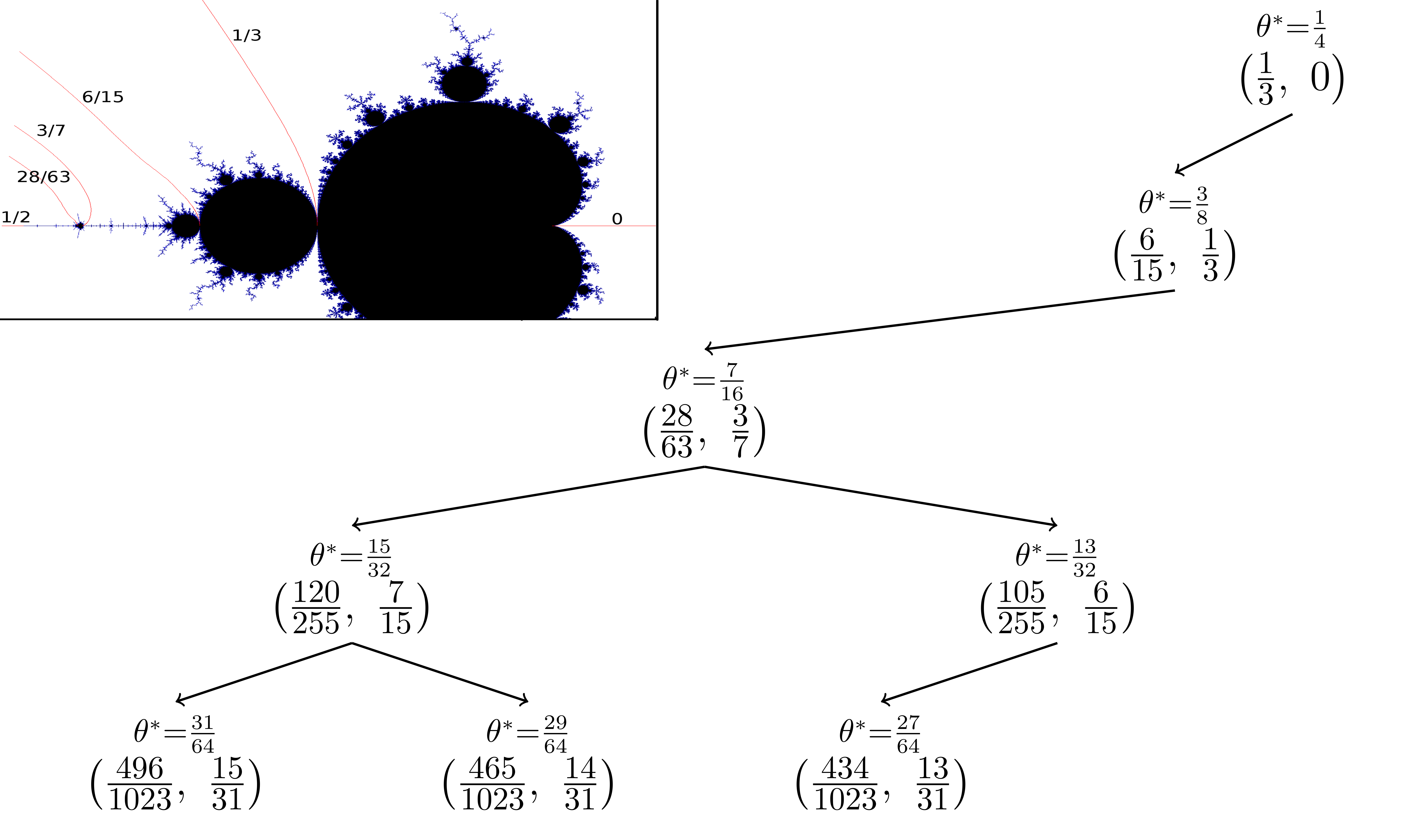
Figure 8. The first few generations of the bisection algorithm which produces all real hyperbolic windows between external angles $0$ and $\frac{1}{2}$. Every interval represents a hyperbolic component, and we display the angles of rays landing at the endpoints as well as the pseudocenter $\theta^{*}$. The root of the tree ($\theta^{*}=\frac{1}{4}$) corresponds to the real slice of the main cardioid, its child is the “basilica” component of period $2$ ($\theta^{*}=\frac{3}{8}$), then $\theta^{*}=\frac{7}{16}$ corresponds to the “airplane” component of period $3$ etc. Some branches of the tree do not appear because some pairs of components have an endpoint in common (due to period doubling).

Proof of Theorem 9.7..

The theorem is a rephrasing, in the language of complex dynamics, of ([BCIT], Proposition 3). Indeed, the set $\Lambda$ of [BCIT] is almost precisely the set $\mathcal{R}$ of real parameter angles; precisely, we have the equality $\mathcal{R}\cap[0,1/2]=\frac{1}{2}\Lambda$ ([BCIT], Proposition 7), and the intervals $J_{d}=(r^{-},r^{+})$ of ([BCIT], Section 4.1) determine exactly the hyperbolic windows $[\alpha_{2},\alpha_{1}]$ defined in the statement of the theorem, via the translation $\alpha_{1}=\frac{r^{-}}{2}$ and $\alpha_{2}=\frac{r^{+}}{2}$. ∎

Example

Suppose we want to find all hyperbolic components between the airplane parameter (of period $3$) and the basilica parameter (of period $2$). The ray landing on the root of the airplane component has angle $\theta_{1}=\frac{3}{7}$, while the ray landing immediately to the left of the basilica has angle $\theta_{2}=\frac{2}{5}$. Let us apply the algorithm:

$$\begin{array}[]{lll}\theta_{2}=\frac{2}{5}&=&0.011001100110\dots\\ \theta_{1}=\frac{3}{7}&=&0.011011011011\dots\\ \hline\cr\\ \theta^{*}&=&0.01101\end{array}$$

hence $\alpha_{1}=0.\overline{0110}=\frac{2}{5}$ and $\alpha_{2}=0.\overline{01101001}=\frac{7}{17}$ and we get the component of period $4$ which is the doubling of the basilica. Note we do not always get the doubling of the previous component; indeed, the next step would be

$$\begin{array}[]{lll}\theta_{2}=\frac{7}{17}&=&0.011010010110\dots\\ \theta_{1}=\frac{3}{7}&=&0.011011011011\dots\\ \hline\cr\\ \theta^{*}&=&0.011011\end{array}$$

hence $\alpha_{1}=0.\overline{01101}$ and we get a component of period $5$. Iteration of the algorithm produces all real hyperbolic components. We conjecture that a similar algorithm holds in every vein.

10. A copy of the Hubbard tree inside parameter space

We saw that the set of rays which land on the real axis in parameter space also land in the dynamical plane. In order to establish equality of dimensions, we would like to prove the other inclusion. Unfortunately, in general there is no copy of $H_{c}$ inside $P_{c}$ (for instance, is $c$ is the basilica tuned with itself, then the Hubbard tree is a countable set, while only two pairs of rays land in parameter space to the right of $c$). However, outside of the baby Mandelbrot sets, one can indeed map the combinatorial model for the Hubbard tree into the combinatorial model of parameter space:

Proposition 10.1.

Given a non-renormalizable, real parameter $c$ and another real parameter $c^{\prime}>c$, there exists a piecewise linear map $F:\mathbb{R}/\mathbb{Z}\to\mathbb{R}/\mathbb{Z}$ such that

$$F(H_{c^{\prime}})\subseteq P_{c}.$$

Proof.

Let us denote $\ell:=\ell(c)$ and $\ell^{\prime}:=\ell(c^{\prime})$ the lengths of the characteristic leaves. Let us now choose a dominant parameter $c^{\prime\prime}$ in between $c$ and $c^{\prime}$ and such that its corresponding string $w_{c^{\prime\prime}}=\overline{S}$ with $S$ dominant, in such a way that $S$ is a prefix of $w_{c}$ and not a prefix of $w_{c^{\prime}}$. Let us denote by $\ell^{\prime\prime}:=\ell(c^{\prime\prime})$ the length of the characteristic leaf of $c^{\prime\prime}$.

If $S=(s_{1},s_{2},\dots,s_{n})$ (recall $n$ must be even), let us define the dyadic number

$$s:=0.01^{s_{1}}0^{s_{2}}\dots 1^{s_{n-1}}0^{s_{n}}$$

and the “length” of $S$ to be $N:=s_{1}+s_{2}+\dots+s_{n}$. Then, let us construct the map

(4) $$F(\theta):=\left\{\begin{array}[]{ll}s+\frac{1-\theta}{2^{N+1}}&\textup{ if }0\leq\theta<\frac{1}{2}\\ (1-s)+\frac{\theta}{2^{N+1}}&\textup{ if }\frac{1}{2}\leq\theta<1\\ \end{array}\right.$$

Let us now check that $F$ maps $[0,\frac{1}{2})\cap H_{c^{\prime}}$ into $P_{c^{\prime\prime}}\subseteq P_{c}$ (then the other half follows by symmetry). In order to verify the claim, let us pick $\theta\in H_{c^{\prime}}$, $0<\theta<\frac{1}{2}$. We need to check that $\phi:=F(\theta)$ satisfies:

1. $\ell(\phi)\leq\ell^{\prime\prime}$;

2. $T^{n}(\ell(\phi))\leq\ell(\phi)\qquad\forall n\geq 0$.

(1) Since $\theta$ belongs to $H_{c^{\prime}}$, by Proposition 8.3 we have

$$\ell(\theta)\geq L_{c^{\prime}}\geq L_{c^{\prime\prime}}.$$

Moreover, equation (4) implies

$$\ell(\phi)=2s+2^{-N}(1-\ell(\theta)/2)$$

while by the definition of $s$ one has

$$\ell^{\prime\prime}=2s+2^{-N}(1-L_{c^{\prime\prime}}/2)$$

hence combining with the previous inequality we get $\ell(\phi)\leq\ell^{\prime\prime}$.

(2) If $1\leq n<N$, then either $T^{n}(\ell(\phi))\leq\frac{1}{2}<\ell(\phi)$, or $T^{n}(\ell(\phi))$ is of the form

$$0.1^{s_{k}}0^{s_{k+1}}\dots 0^{s_{n}}\dots$$

which is less than $0.1^{s_{1}}0^{s_{2}}\dots 1^{s_{n}}$ because of dominance. If instead $n>N$, $T^{n}(\ell(\phi))=T^{n-N-1}(\ell(\theta))\leq\ell^{\prime}$, and $\ell^{\prime}<\ell(\phi)$ because $\ell(\phi)$ begins with $0.1^{s_{1}}0^{s_{2}}\dots 0^{s_{n}}$, and $S$ is not a prefix of $w_{\theta^{\prime}}$. Finally, let $\hat{\theta}:=\max\{\theta,1-\theta\}$ and analyze the $N^{th}$ iterate: we have

$$T^{N}(\ell(\phi))=\hat{\theta}\leq 2s+\frac{\hat{\theta}}{2^{N}}=\ell(\phi)$$

because $\hat{\theta}$ belongs to $H_{c^{\prime}}\subseteq H_{c^{\prime\prime}}$, and $\max\{\theta\in[0,1]\ :\theta\in H_{c^{\prime\prime}}\}=2s/(1-2^{-N})$. ∎

11. Renormalization and tuning

The Mandelbrot set has the remarkable property that near every point of its boundary there are infinitely many copies of the whole $\mathcal{M}$, called baby Mandelbrot sets. A hyperbolic component $W$ of the Mandelbrot set is a connected component of the interior of $\mathcal{M}$ such that all $c\in W$, the orbit of the critical point is attracted to a periodic cycle under iteration of $f_{c}$.

Douady and Hubbard [DH] related the presence of baby copies of $\mathcal{M}$ to renormalization in the family of quadratic polynomials. More precisely, they associated to any hyperbolic component $W$ a tuning map $\iota_{W}:\mathcal{M}\rightarrow\mathcal{M}$ which maps the main cardioid of $\mathcal{M}$ to $W$, and such that the image of the whole $\mathcal{M}$ under $\iota_{W}$ is a baby copy of $\mathcal{M}$.

The tuning map can be described in terms of external angles in the following terms [Do1]. Let $W$ be a hyperbolic component, and $\eta_{0}$, $\eta_{1}$ the angles of the two external rays which land on the root of $W$. Let $\eta_{0}=0.\overline{\Sigma_{0}}$ and $\eta_{1}=0.\overline{\Sigma_{1}}$ be the (purely periodic) binary expansions of the two angles which land at the root of $W$. Let us define the map $\tau_{W}:\mathbb{R}/\mathbb{Z}\rightarrow\mathbb{R}/\mathbb{Z}$ in the following way:

$$\theta=0.\theta_{1}\theta_{2}\theta_{3}\dots\mapsto\tau_{W}(\theta)=0.\Sigma_{\theta_{1}}\Sigma_{\theta_{2}}\Sigma_{\theta_{3}}\dots$$

where $\theta=0.\theta_{1}\theta_{2}\dots$ is the binary expansion of $\theta$, and its image is given by substituting the binary string $\Sigma_{0}$ to every occurrence of $0$ and $\Sigma_{1}$ to every occurrence of $1$.

Proposition 11.1 ([Do3], Proposition 7).

The map $\tau_{W}$ has the property that, if $\theta$ is a characteristic angle of the parameter $c\in\partial\mathcal{M}$, then $\tau_{W}(\theta)$ is a characteristic angle of the parameter $\iota_{W}(c)$.

If $W$ is a real hyperbolic component, then $\iota_{W}$ preserves the real axis. The image of the tuning operator is the tuning window $\Omega(W)$ with

$$\Omega(W):=[\omega(W),\alpha(W)]$$

where

$$\begin{array}[]{lll}\alpha(W)&:=&0.\overline{\Sigma_{0}}\\ \omega(W)&:=&0.\Sigma_{0}\overline{\Sigma_{1}}.\end{array}$$

The point $\alpha(W)$ will be called the root of the tuning window. Overlapping tuning windows are nested, and we call maximal tuning window a tuning window which is not contained in any other tuning window.

Let us describe the behavior of Hausdorff dimension with respect to the tuning operator:

Proposition 11.2.

Let $W$ be a hyperbolic component of period $p$ with root $r(W)$, and let $c\in\mathcal{M}$. Then we have the equalities

$$\textup{H.dim }H_{\tau_{W}(c)}=\max\left\{\textup{H.dim }H_{r(W)},\textup{H.dim }\tau_{W}(H_{c})\right\}$$

$$\textup{H.dim }P_{\tau_{W}(c)}=\max\left\{\textup{H.dim }P_{r(W)},\textup{H.dim }\tau_{W}(P_{c})\right\}.$$

Moreover,

$$\textup{H.dim }\tau_{W}(H_{c})=\frac{1}{p}\textup{H.dim }H_{c}.$$

Proof.

Let $c^{\prime}:=\tau_{W}(c)$. The Julia set of $f_{c^{\prime}}$ is constructed by taking the Julia set of $f_{r(W)}$ and inserting a copy of the Julia set of $f_{c}$ inside every bounded Fatou component. Hence in particular, the extended Hubbard tree of $J(f_{c^{\prime}})$ contains a topological copy $T_{1}$ of the extended Hubbard tree of $f_{r(W)}$ which contains the critical value $c^{\prime}$. The set of angles which land on $T_{1}$ are precisely the image $\tau_{W}(H^{ext}_{c})$ via tuning of the set $H^{ext}_{c}$ of angles which land on the extended Hubbard tree of $H_{c}$. Let $\theta\in H_{c^{\prime}}$ be an angle whose ray lands on the Hubbard tree of $f_{c^{\prime}}$. Then either $\theta$ also belongs to $H_{r(W)}$ or it lands on a small copy of the extended Hubbard tree of $f_{r(W)}$, hence it eventually maps to $T_{1}$. Hence we have the inclusions

$$H_{r(W)}\cup\tau_{W}(H_{c})\subseteq H_{c^{\prime}}\subseteq H_{r(W)}\cup\bigcup_{n\geq 0}D^{-n}(\tau_{W}(H^{ext}_{c}))$$

from which the claim follows, recalling that $H^{ext}_{c}\setminus\{-\beta,\beta\}\subseteq\bigcup_{n\geq 0}D^{-n}(H_{c})$.

In parameter space, one notices that the set of rays landing on the vein $v$ for $c^{\prime}$ either land between $0$ and $r(W)$, or between $r(W)$ and $c^{\prime}$. In the latter case, they land on the small copy of the Mandelbrot set with root $r(W)$, so they are in the image of $\tau_{W}$. Hence

$$P_{c^{\prime}}=P_{r(W)}\cup\tau_{W}(P_{c})$$

and the claim follows. The last claim follows by looking at the commutative diagram

Since $\tau_{W}$ is injective and continuous restricted to $H_{c}$ (because $H_{c}$ does not contain dyadic rationals) we have by Proposition 5.3

$$h_{top}(D,H_{c})=h_{top}(D^{p},\tau_{W}(H_{c}))$$

and, since $H_{c}$ is forward invariant we can apply Proposition 5.5 and get

$$\textup{H.dim }\tau_{W}(H_{c})=\frac{h_{top}(D^{p},\tau_{W}(H_{c}))}{p\log 2}=\frac{1}{p}\frac{h_{top}(D,H_{c})}{\log 2}=\frac{1}{p}\textup{H.dim }H_{c}$$

from which the claim follows.

∎

11.1. Scaling and continuity at the Feigenbaum point

Among all tuning operators is the operator $\tau_{W}$ where $W$ is the basilica component of period $2$ (the associated strings are $\Sigma_{0}=01$, $\Sigma_{1}=10$). We will denote this particular operator simply with $\tau$. The fixed point of $\tau$ is the external angle of the Feigenbaum point $c_{Feig}$.

Let us explicitly compute the dimension at the Feigenbaum parameter. Indeed, let $c_{0}$ be the airplane parameter of angle $\theta_{0}=3/7$, and consider the sequence of parameters of angles $\theta_{n}:=\tau^{n}(\theta_{0})$ given by successive tuning.

The set $H_{c_{0}}$ is given by all angles with binary sequences which do not contain $3$ consecutive equal symbols, hence the Hausdorff dimension is easily computable (see example 4 in the introduction):

$$\textup{H.dim }H_{\theta_{0}}=\log_{2}\frac{\sqrt{5}+1}{2}.$$

Now, by repeated application of Proposition 11.2 we have

$$\textup{H.dim }H_{\theta_{n}}=\frac{\textup{H.dim }H_{\theta_{0}}}{2^{n}}.$$

Note that the angles $\theta_{n}$ converge from above to the Feigenbaum angle $\theta_{F}$, also $\textup{H.dim }H_{c_{Feig}}=0$; moreover, since $\theta_{n}$ is periodic of period $2^{n}$,

$$\theta_{n}-\theta_{F}\asymp 2^{-2^{n}}$$

and together with

(5) $$\textup{H.dim }H_{\theta_{n}}-\textup{H.dim }H_{\theta_{F}}=\frac{\textup{H.dim }H_{\theta_{0}}}{2^{n}}$$

we have proved the

Proposition 11.3.

For the Feigenbaum parameter $c_{Feig}$ we have

$$\textup{H.dim }S_{c_{Feig}}=0$$

and moreover, the entropy function $\theta\mapsto h(\theta)$ is not Hölder-continuous at the Feigenbaum point. Similarly, the dimension of the set of biaccessible angles for the Feigenbaum parameter is $0$.

Note that it also follows that the entropy $h(c):=h_{top}(f_{c},[-\beta,\beta])$ as a function of the parameter $c$ has vertical tangent at $c=c_{Feig}$, as shown in Figure 1. Indeed, if $c_{n}\to c_{Feig}$ is the sequence of period doubling parameters converging to the Feigenbaum point, it is a deep result [Ly2] that $|c_{n}-c_{Feig}|\asymp\lambda^{-n}$, where $\lambda\cong 4.6692\dots$ is the Feigenbaum constant; hence, by equation (5), we have

$$\frac{h(c_{n})-h(c_{Feig})}{|c_{n}-c_{Feig}|}\asymp\left(\frac{\lambda}{2}\right)^{n}\to\infty.$$

11.2. Proof of Theorem 1.7

Let us now turn to the proof of equality of dimensions between $H_{c}$ and $P_{c}$. Recall we already established $P_{c}\subseteq H_{c}$, hence we are left with proving that for all real parameters $c\in\partial\mathcal{M}\cap\mathbb{R}$,

$$\textup{H.dim }H_{c}\leq\textup{H.dim }P_{c}.$$

By Proposition 11.3, the inequality holds for the Feigenbaum point and for all $c>c_{Feig}$. Moreover, by Proposition 10.1 and continuity of entropy ([MT], see also section 13), we have the inequality for any $c\in\partial\mathcal{M}\cap\mathbb{R}$ which is non-renormalizable. Let now $\tau$ be the tuning operator whose fixed point is the Feigenbaum point: since the root of its tuning window is the basilica map which has zero entropy, by Proposition 11.2 we have, for each $n\geq 0$ and each $c\in\mathcal{M}$,

(6) $$\textup{H.dim }H_{\tau^{n}(c)}=\textup{H.dim }\tau^{n}(H_{c})\qquad\textup{H.dim }P_{\tau^{n}(c)}=\textup{H.dim }\tau^{n}(P_{c}).$$

Now, each renormalizable parameter $c\in\mathcal{M}\cap(-2,c_{Feig})$ is either of the form $c=\tau^{n}(c_{0})$ with $c_{0}$ non-renormalizable, or $c=\tau^{n}(\tau_{W}(c_{0}))$ with $W$ a real hyperbolic component such that its root $r(W)$ is outside the baby Mandelbrot set determined by the image of $\tau$.

1. In the first case we note that (since tuning operators behave well under the operation of concatenation of binary strings), by applying the operator $\tau^{n}$ to both sides of the inclusion of Proposition 10.1 we get for each $c^{\prime}>c_{0}$ a piecewise linear map $F_{0}$ such that

   $$F_{0}(\tau^{n}(H_{c^{\prime}}))\subseteq\tau^{n}(P_{c_{0}})$$

   hence, by continuity of entropy and of tuning operators,

   $$\textup{H.dim }H_{c}=\sup_{c^{\prime}>c_{0}}\textup{H.dim }H_{\tau^{n}(c^{\prime})}=\textup{H.dim }\tau^{n}(H_{c^{\prime}})\leq\textup{H.dim }\tau^{n}(P_{c_{0}})=\textup{H.dim }P_{c}.$$

2. In the latter case $c=\tau^{n}(\tau_{W}(c_{0}))$, by Proposition 11.2 we get

   $$\tau^{n}(P_{\tau_{W}(c_{0})})=\tau^{n}(P_{r(W)})\cup\tau^{n}(\tau_{W}(P_{c_{0}}))$$

   and since the period of $W$ is larger than $2$ we have the inequality

   $$\textup{H.dim }\tau^{n}(\tau_{W}(P_{c_{0}}))\leq\textup{H.dim }\tau^{n+1}(P_{c_{0}})\leq\textup{H.dim }\tau^{n+1}(\mathcal{R})\leq\tau^{n}(P_{r(W)})$$

   where in the last inequality we used the fact that the set of rays $\tau(\mathcal{R})$ land to the right of the root $r(W)$. Thus we proved that

   $$\textup{H.dim }\tau^{n}(P_{\tau_{W}(c_{0})})=\textup{H.dim }\tau^{n}(P_{r(W)})$$

   and the same reasoning for $H_{c}$ yields

   $$\textup{H.dim }\tau^{n}(H_{\tau_{W}(c_{0})})=\textup{H.dim }\tau^{n}(H_{r(W)}).$$

   Finally, putting together the previous equalities with eq.(6) and applying the case (1) to $\tau^{n}(r(W))$ (recall $r(W)$ is non-renormalizable), we have the equalities

   $$\textup{H.dim }P_{c}=\textup{H.dim }\tau^{n}(P_{\tau_{W}(c_{0})})=\textup{H.dim }\tau^{n}(P_{r(W)})=\textup{H.dim }P_{\tau^{n}(r(W))}=$$

   $$=\textup{H.dim }H_{\tau^{n}(r(W))}=\textup{H.dim }\tau^{n}(H_{r(W)})=\textup{H.dim }\tau^{n}(H_{\tau_{W}(c_{0})})=\textup{H.dim }H_{c}.$$

11.3. Density of dominant parameters

In order to prove Proposition 9.6, we will need the following definitions: given a string $S$, the set of its prefixes-suffixes is

$$\begin{array}[]{lll}PS(S)&:=&\{Y:Y\textup{ is both a prefix and a suffix of }S\}=\\ &=&\{Y:Y\neq\emptyset,\exists\ X,Z\textup{ s.t. }S=XY=YZ\}.\end{array}$$

Note that an extremal string $S$ of even length is dominant if and only if $PS(S)$ is empty. Moreover, let us define the set of residual suffixes as

$$RS(S):=\{Z\ :\ S=YZ,\ Y\in PS(S)\}.$$

Proof of Proposition 9.6. By density of the roots of the maximal tuning windows in the set of non-renormalizable angles, it is enough to prove that every $\theta\in(0,\frac{1}{2})$ which is root of a maximal tuning window, $\theta\neq 1/3$, can be approximated from the right by dominant points. Hence we can assume $w_{\theta}=\overline{S}$, $S$ an extremal string of even length, and $1$ is not a prefix of $S$. If $S$ is dominant, a sequence of approximating dominant parameters is given by the strings

$$S^{n}11,\qquad n\geq 1.$$

The rest of the proof is by induction on $|S|$. If $|S|=2$, then $S$ itself is dominant and we are in the previous case. If $|S|>2$, either $S$ is dominant and we are done, or $PS(S)\neq\emptyset$ and also $RS(S)\neq\emptyset$. Let us choose $Z_{\star}\in RS(S)$ such that

$$\overline{Z_{\star}}:=\min\{\overline{Z}\ :\ Z\in RS(S)\}$$

and $Y_{\star}\in PS(S)$ such that $S=Y_{\star}Z_{\star}$. Let $\alpha(Y_{\star})$ be the root of the maximal tuning window $\overline{Y_{\star}}$ belongs to. Then by Lemma 11.7, $\overline{Z_{\star}}>\alpha(Y_{\star})$, and by minimality

$$\alpha(Y_{\star})<\overline{Z}\quad\forall Z\in RS(S).$$

Now, since $Y_{\star}$ has odd length and belongs to the window of root $\alpha(Y_{\star})$, then one can write $\alpha(Y_{\star})=\overline{P}$ with $Y_{\star}<<P$, hence also $S<<P$. Moreover,

$$|P|\leq|Y_{\star}|+1\leq|S|$$

and actually $|Y_{\star}|+1<|S|$ because otherwise the first digit of $Y_{\star}$ would appear twice at the beginning of $S$, contradicting the fact that $S$ is extremal. Suppose now $\alpha(Y_{\star})\neq\overline{1}$. Then $|P|<|S|$ and by induction there exists $\gamma=\overline{T}$ such that $T$ is dominant,

$$\alpha(Y_{\star})<\overline{T}<\overline{Z}\quad\forall Z\in RS(S)$$

and $\gamma$ can also be chosen close enough to $\alpha(Y_{\star})$ so that $P$ is prefix of $T$, which implies

$$S<<T.$$

By Lemma 11.5, $S^{n}T^{m}$ is a dominant string for $m$ large enough, of even length if $m$ is even, and arbitrarily close to $\overline{S}$ as $n$ tends to infinity. If $\alpha(Y_{\star})=\overline{1}$, the string $S^{n}1^{2m}$ is also dominant for $n$, $m$ large enough. ∎

Lemma 11.4.

If $S$ is an extremal string and $Y\in PS(S)$, then $Y$ is an extremal string of odd length.

Proof.

Suppose $S=XY=YZ$. Then by extremality $XY<YX$, hence $XYY<YXY$ and, by substituting $YZ$ for $XY$, $YZY<YYZ$. If $|Y|$ were even, it would follow that $ZY<YZ$, which contradicts the extremality of $S=YZ<ZY$. Hence $|Y|$ is odd. Suppose now $Y=AB$, with $A$ and $B$ non-empty strings. Then $S=XAB<BXA$. By considering the first $k:=|Y|$ characters on both sides of this equation, $Y=AB=S_{1}^{k}\leq(BXA)_{1}^{k}=BA$. If $Y=AB=BA$, then $Y=P^{k}$ for some string $P$, hence by Lemma 9.1 we have $PZP^{k-1}<P^{k}Z=S$, which contradicts the extremality of $S$, hence $AB<BA$ and $Y$ is extremal. ∎

Lemma 11.5.

Let $S$ be an extremal string of even length, and $T$ be a dominant string. Suppose moreover that

1. $S<<T$;

2. $\overline{T}<\overline{Z}$ $\ \forall Z\in RS(S)$.

Then, for any $n\geq 1$ and for $m$ sufficiently large, $S^{n}T^{m}$ is a dominant string.

Proof.

Let us check that $S^{n}T^{m}$ by checking all its splittings. We have four cases:

1. From (1), we have

   $$S^{n}T^{m}<<T^{a},\quad a\geq 1$$

   $$S^{n}T^{m}<<S^{b}T^{m},\quad b<n.$$

2. If $S=XY$, $XY<<YX$ by extremality, hence

   $$S^{n}T^{m}<<YS^{b}T^{m}\quad\forall b\geq 1.$$

3. Since $T$ is dominant, $T<<U$ whenever $T=QU$, thus

   $$S^{n}T^{m}<<T<<U.$$

4. One is left to prove that $S^{n}T^{m}<<YT^{m}$ whenever $S=XY$. If $Y\notin PS(S)$, then $XY<<Y$ and the proof is complete. Otherwise, $S=XY=YZ$, $|Y|\equiv 1\mod 2$ by Lemma 11.4. Moreover, since $YZ<ZY$, by a few repeated applications of Lemma 9.1, we have $\overline{ZS^{n-1}}>\overline{Z}$, hence (2) implies $\overline{T}<\overline{ZS^{n-1}}$, and by Lemma 11.6 we have $ZS^{n-1}\overline{T}>\overline{T}$, hence for $m$ large enough $ZS^{n-1}T^{m}>>T^{m}$ and then

   $$S^{n}T^{m}<<YT^{m}.$$

∎

Lemma 11.6.

Let $Y$, $Z$ be finite strings of positive integers such that $\overline{Y}<\overline{Z}$. Then

$$Z\overline{Y}>\overline{Y}.$$

Proof.

By Lemma 9.1, for any $k\geq 0$ we have

$$\overline{Y^{k}}<\overline{Z}\Rightarrow Y^{k}Z<ZY^{k}$$

hence, by taking the limit as $k\to\infty$, $Z\overline{Y}\geq\overline{Y}$. Equality cannot hold because otherwise $Y$ and $Z$ have to be multiple of the same string, which contradicts the strict inequality $\overline{Y}<\overline{Z}$. ∎

Lemma 11.7.

Let $\theta$ be a non-renormalizable, real parameter angle such that $w_{\theta}=\overline{S}$ and $S$ is an extremal string of even length, and let $Y\in PS(S)$, $S=YZ$. Let $\phi$ the parameter angle such that $w_{\phi}=\overline{Y}$, and let $\Omega=[\omega,\alpha]$ be the maximal tuning window which contains $\phi$. Then if $w_{\alpha}=\overline{S_{0}}$, we have

$$\overline{Z}>\overline{S_{0}}.$$

Proof.

Since $\phi$ lies in the tuning window $\Omega$, $Y$ is a concatenation of the strings $S_{0}$ and $S_{1}$. As a consequence, $Y\overline{S_{0}}$ is also a concatenation of strings $S_{0}$ and $S_{1}$, so $Y\overline{S_{0}}\geq S_{1}\overline{S_{0}}$. Moreover, by Lemma 9.1, $\overline{S}<\overline{Y}<\overline{S_{0}}$. We now claim that

$$\beta:=\overline{ZY}>\overline{S_{0}}.$$

Indeed, suppose $\beta\leq\overline{S_{0}}$; then, $\overline{S}=Y\beta\geq Y\overline{S_{0}}\geq S_{1}\overline{S_{0}}$, which combined with the fact that $\overline{S}<\overline{S_{0}}$ implies $\theta$ lies in the tuning window $\Omega$, contradicting the fact that $\theta$ is non-renormalizable.

Now, suppose $\overline{Z}\leq\overline{S_{0}}$; then $\overline{Z}\leq\overline{S_{0}}\leq\overline{ZY}$, which implies $Z$ has to be prefix of $\overline{S_{0}}$, hence $Z=S_{0}^{k}V$ with $V$ prefix of $S_{0}$, $V\neq\emptyset$ since $|Z|$ is odd. If $S_{0}\neq(1,1)$, then $S_{0}$ is extremal and, by Lemma 9.1, $\overline{Z}=\overline{S_{0}^{k}V}>\overline{S_{0}}$, contradiction. In the case $S_{0}=(1,1)$, then $Z$ must be just a sequence of $1$’s of odd length, which forces $\overline{S}=\overline{1}$, hence $S$ cannot be extremal. ∎

12. The complex case

In the following sections we will develop in detail the tools needed to prove Theorem 1.3. In particular, in section 13 we prove continuity of entropy along principal veins by developing a generalization of kneading theory to tree maps. Then (section 14) we develop the combinatorial surgery map, which maps the combinatorial model of real Hubbard trees to Hubbard trees along the vein. Finally (section 14.5), we use the surgery to transfer the inclusion of Hubbard tree in parameter space of section 10 from the real vein to the other principal veins.

12.1. Veins

A vein in the Mandelbrot set is a continuous, injective arc inside $\mathcal{M}$. Branner and Douady [BD] showed that there exists a vein joining the parameter at angle $\theta=1/4$ to the main cardiod of $\mathcal{M}$. In his thesis, J. Riedl [Ri] showed existence of veins connecting any tip at a dyadic angle $\theta=\frac{p}{2^{q}}$ to the main cardioid. Another proof of this fact is due to J. Kahn (see [Do2], Section V.4, and [Sch], Theorem 5.6). Riedl also shows that the quasiconformal surgery preserves local connectivity of Julia sets, hence by using the local connectivity of real Julia sets [LvS] one concludes that all Julia sets of maps along the dyadic veins are locally connected ([Ri], Corollary 6.5) .

Let us now see how to define veins combinatorially just in terms of laminations. Recall that the quadratic minor lamination $QML$ is the union of all minor leaves of all invariant laminations corresponding to all quadratic polynomials. The degenerate leaf $\{0\}$ is the natural root of $QML$. No other leaf of $QML$ contains the angle $0$ as its endpoint. Given a rooted lamination, we define a partial order on the set of leaves by saying that $\ell_{1}<\ell_{2}$ if $\ell_{1}$ separates $\ell_{2}$ from the root.

Definition 12.1.

Let $\ell$ be a minor leaf. Then the combinatorial vein defined by $\ell$ is the set

$$P(\ell):=\{\ell^{\prime}\in QML\ :\{0\}<\ell^{\prime}\leq\ell\}$$

of leaves which separate $\ell$ from the root of the lamination.

12.2. Principal veins

Let $\frac{p}{q}$ be a rational number, with $0<p<q$ and $p,q$ coprime. The $\frac{p}{q}$-limb in the Mandelbrot set is the set of parameters which have rotation number $\frac{p}{q}$ around the $\alpha$ fixed point. In each limb, there exists a unique parameter $c=c_{p/q}$ such that the critical point maps to the $\beta$ fixed point after exactly $q$ steps, i.e. $f^{q}_{c}(0)=\beta$. For instance, $c_{1/2}=-2$ is the Chebyshev polynomial. These parameters represent the “highest antennas” in the limbs of the Mandelbrot set. The principal vein $v_{p/q}$ is the vein joining $c_{p/q}$ to the main cardioid. We shall denote by $\tau_{p/q}$ the external angle of the ray landing at $c_{p/q}$ in parameter space.

Proposition 12.2.

Each parameter $c\in v_{p/q}$ is topologically finite, and the Hubbard tree $T_{c}$ is a $q$-pronged star. Moreover, the valence of any point $x\in T_{c}$ is at most $2q$.

Proof.

Let $\tau$ be the point in the Julia set of $f_{c}$ where the ray at angle $\tau_{p/q}$ lands. Since $c\in[\alpha,\tau]$, then $f^{q-1}(c)\in[\alpha,\beta]$, hence by Lemma 4.4 the extended Hubbard tree is a $q$-pronged star. The unique point with degree larger than $1$ is the $\alpha$ fixed point, which has degree $q$, so the second claim follows from Lemma 4.8. ∎

Note that, by using combinatorial veins, the statement of Theorem 1.3 can be given in purely combinatorial form as follows. Given a set $\lambda$ of leaves in the unit disk, let us denote by $\textup{H.dim }\lambda$ the Hausdorff dimension of the set of endpoints of (non-degenerate) leaves of $\lambda$. Moreover, if the leaf $\ell$ belongs to $QML$ we shall denote as $\lambda(\ell)$ the invariant quadratic lamination which has $\ell$ as minor leaf. The statement of the theorem then becomes that, for each $\ell\in P(\tau_{p/q})$, the following equality holds:

$$\textup{H.dim }P(\ell)=\textup{H.dim }\lambda(\ell).$$

We conjecture that the same equality holds for every $\ell\in QML$.

12.3. A combinatorial bifurcation measure

The approach to the geometry of the Mandelbrot set via entropy of Hubbard trees allows one to define a transverse measure on the quadratic minor lamination $QML$. Let $\ell_{1}<\ell_{2}$ be two ordered leaves of $QML$, corresponding to two parameters $c_{1}$ and $c_{2}$, and let $\gamma$ be a tranverse arc connecting $\ell_{1}$ and $\ell_{2}$. Then one can assign the measure of the arc $\gamma$ to be the difference between the entropy of the two Hubbard trees:

$$\mu(\gamma):=h(f_{c_{2}}\mid_{T_{c_{2}}})-h(f_{c_{1}}\mid_{T_{c_{1}}}).$$

By the monotonicity result of [TaoL], such a measure can be interpreted as a transverse bifurcation measure: in fact, as one crosses more and more leaves from the center of the Mandelbrot set to the periphery, i.e. as the map $f_{c}$ undergoes more and more bifurcations, one picks up more and more measure. The measure can also be interpreted as the derivative of the entropy in the direction transverse to the leaves: note also that, since period doubling bifurcations do not change the entropy, $\mu$ is non-atomic.

The dual to the lamination is an $\mathbb{R}$-tree, and the transverse measure $\mu$ defines a metric on such a tree. By pushing it forward to the actual Mandelbrot set, one endows the union of all veins in $\mathcal{M}$ with the structure of a metric $\mathbb{R}$-tree. It would be very interesting to analyze the properties of such transverse measure, and also comparing it to the other existing notions of bifurcation measure.

In the following sections we will develop the proof of Theorem 1.3.

13. Kneading theory for Hubbard trees

In this section we will analyze the symbolic dynamics of some continuous maps of trees, in order to compute their entropy as zeros of some power series. As a consequence, we will see that the entropy of Hubbard trees varies continuously along principal veins. Our work is a generalization to tree maps of Milnor and Thurston’s kneading theory [MT] for interval maps. The general strategy is similar to [BdC], but our view is towards application to Hubbard trees. Moreover, since we are mostly interested in principal veins, we will treat in detail only the case of trees with a particular topological type. An alternative, independent approach to continuity is in [BS].

13.1. Counting laps and entropy

Let $f:T\to T$ be a continuous map of a finite tree $T$. We will assume $f$ is a local homeomorphism onto its image except at one point, which we call the critical point. At the critical point, the map is a branched cover of degree $2$. Let us moreover assume $T$ is a rooted tree, i.e. it has a distinguished end $\beta$. The choice of a root defines a partial ordering on the tree; namely, $x<y$ if $x$ disconnects $y$ from the root.

Let $C_{f}$ be a finite set of points of $T$ such that $T\setminus C_{f}$ is a union of disjoint open intervals $I_{k}$, and the map $f$ is monotone on each $I_{k}$ with respect to the above-mentioned ordering. The critical point and the branch points of the tree are included in $C_{f}$.

For each subtree $J\subseteq T$, the number of laps of the restriction of $f^{n}$ to $J$ is defined as $\ell(f^{n}\mid_{J}):=\#(J\cap\bigcup_{i=0}^{n-1}f^{-i}(C_{f}))+\#\textup{Ends}(J)-1$, in analogy with the real case. Denote $\ell(f^{n}):=\ell(f^{n}\mid_{T})$. The growth number $s$ of the map $f:T\to T$ is the exponential growth rate of the number of laps:

(7) $$s:=\lim_{n\to\infty}\sqrt[n]{\ell(f^{n})}.$$

Lemma 13.1 ([BdC], Lemma 4.1).

The limit in eq. (7) exists, and it is related to the topological entropy $h_{top}(f\mid_{T})$ in the following way:

$$s=e^{h_{top}(f\mid_{T})}.$$

The proof is the same as in the analogous result of Misiurewicz and Szlenk for interval maps ([dMvS], Theorem II.7.2). In order to compute the entropy of $f$, let us define the generating function

$$\mathcal{L}(t):=1+\sum_{n=1}^{\infty}\ell(f^{n})t^{n}$$

where $\ell(f^{n})$ is the number of laps of $f^{n}$ on all $T$. Moreover, for $a,b\in T$, let us denote as $\ell(f^{n}\mid_{[a,b]})$ the number of laps of the restriction of $f^{n}$ to the interval $[a,b]$. Thus we can construct for each $x\in T$ the function

$$\mathcal{L}(x,t):=1+\sum_{n=1}^{\infty}\ell(f^{n}\mid_{[\beta,x]})t^{n}$$

and for each $n$ we shall denote $L_{n,x}:=\ell(f^{n}\mid_{[\beta,x]})$. Let us now relate the generating function $\mathcal{L}$ to the kneading sequence.

Before doing so, let us introduce some notation; for $x\notin C_{f}$, the sign $\epsilon(x)\in\{\pm 1\}$ is defined according as to whether $f$ preserves or reverses the orientation of a neighbourhood of $x$. Finally, let us define

$$\eta_{k}(x):=\epsilon(x)\cdots\epsilon(f^{k-1}(x))$$

for $k\geq 1$, and $\eta_{0}(x):=1$. Moreover, let us introduce the notation

$$\chi_{k}(x):=\left\{\begin{array}[]{ll}1&\textup{if }f(x)\in I_{k}\\ 0&\textup{if }f(x)\notin I_{k}\end{array}\right.$$

and $\hat{\chi}_{k}(x):=1-\chi_{k}(x)$.

Let us now focus on the case when $T$ is the Hubbard tree of a quadratic polynomial along the principal vein $v_{p/q}$. Then we can set $C_{f}:=\{\alpha,0\}$ the union of the $\alpha$ fixed point and the critical point, so that

$$T\setminus C_{f}=I_{0}\cup I_{1}\cup\dots\cup I_{q}$$

where the critical point separates $I_{0}$ and $I_{1}$, and the $\alpha$ fixed point separates $I_{1},I_{2},\dots,I_{q}$. The dynamics is the following:

• $f:I_{k}\mapsto I_{k+1}$ homeomorphically, for $1\leq k\leq q-1$;

• $f:I_{q}\mapsto I_{0}\cup I_{1}$ homeomorphically;

• $f(I_{0})\subseteq I_{0}\cup I_{1}\cup I_{2}$.

We shall now write a formula to compute the entropy of $f$ on the tree as a function of the itinerary of the critical value.

Proposition 13.2.

Suppose the critical point for $f$ is not periodic. Then we have the equality

$$\mathcal{L}(c,t)\left[1-2t\Theta_{1}(t)+\frac{4t^{2}}{1+t}\Theta_{2}(t)\right]=\Theta_{3}(t)$$

as formal power series, where

$$\Theta_{1}(t):=\sum_{k=0}^{\infty}\eta_{k}(c)\hat{\chi}_{0}(f^{k}(c))t^{k}$$

$$\Theta_{2}(t):=\sum_{k=0}^{\infty}\eta_{k}(c)\chi_{2}(f^{k}(c))t^{k}$$

depend only on the itinerary of the critical value $c$, and $\Theta_{3}(t)$ is some power series with real, non-negative, bounded coefficients. (Note that, in order to deal with the prefixed case, we extend the definitions of $\epsilon$, $\hat{\chi}_{0}$ and $\chi_{2}$ by setting $\epsilon(\alpha)=\hat{\chi}_{0}(\alpha)=\chi_{2}(\alpha)=1$.)

Proof.

We can compute the number of laps recursively. Let us suppose $x\in T$ such that $f^{n}(x)\neq 0$ for all $n\geq 0$. Then for $n\geq 2$ we have the following formulas:

$$\ell(f^{n}\mid_{[\beta,x]})=\left\{\begin{array}[]{ll}\ell(f^{n-1}\mid_{[\beta,f(x)]})&\textup{if }x\in I_{0}\cup\{0\}\\ -\ell(f^{n-1}\mid_{[\beta,f(x)]})+2\ell(f^{n-1}\mid_{[\beta,c]})+1&\textup{if }x\in I_{1}\\ \ell(f^{n-1}\mid_{[\beta,f(x)]})+2\ell(f^{n-1}\mid_{[\beta,c]})-2\ell(f^{n-1}\mid_{[\beta,\alpha]})&\textup{if }x\in I_{2}\cup\dots\cup I_{q-1}\cup\{\alpha\}\\ -\ell(f^{n-1}\mid_{[\beta,f(x)]})+2\ell(f^{n-1}\mid_{[\beta,c]})+1&\textup{if }x\in I_{q}\end{array}\right.$$

Now, recalling the notation $L_{n,x}:=\ell(f^{n}\mid_{[\beta,x]})$, the previous formula can be rewritten as

$$L_{n,x}=\epsilon(x)L_{n-1,f(x)}+2\hat{\chi}_{0}(x)L_{n-1,c}-2\chi_{2}(x)L_{n-1,\alpha}+\frac{1-\epsilon(x)}{2}.$$

Moreover, for $n=1$ we have

$$L_{1,x}=\epsilon(x)+2\hat{\chi}_{0}(x)+\frac{1-\epsilon(x)}{2}+R(x)$$

where

$$R(x):=\left\{\begin{array}[]{ll}1&\textup{if }x\in I_{q}\\ -1&\textup{if }x=\alpha\\ 0&\textup{otherwise.}\end{array}\right.$$

Hence by multiplying every term by $t^{n}$ and summing up we get

$$\mathcal{L}(x,t)=t\epsilon(x)\mathcal{L}(f(x),t)+2t\hat{\chi}_{0}(x)\mathcal{L}(c,t)-2t\chi_{2}(x)\tilde{\mathcal{L}}(\alpha,t)+S(x,t)$$

with $S(x,t):=\frac{1-\epsilon(x)}{2}\frac{t}{1-t}+tR(x)+1$. If we now apply the formula to $f^{k}(x)$ and multiply everything by $\eta_{k}(x)t^{k}$ we have for each $k\geq 0$

$$\eta_{k}(x)t^{k}\mathcal{L}(f^{k}(x),t)-\eta_{k}(x)\epsilon(f^{k}(x))t^{k+1}\mathcal{L}(f^{k+1}(x),t)=$$

$$=2t^{k+1}\eta_{k}(x)\hat{\chi}_{0}(f^{k}(x))\mathcal{L}(c,t)-2t^{k+1}\eta_{k}(x)\chi_{2}(f^{k}(x))\tilde{\mathcal{L}}(\alpha,t)+\eta_{k}(x)t^{k}S(f^{k}(x),t)$$

so, by summing over all $k\geq 0$, the left hand side is a telescopic series and we are left with

(8) $$\mathcal{L}(x,t)=2t\Theta_{1}(x,t)\mathcal{L}(c,t)-2t\Theta_{2}(x,t)\tilde{\mathcal{L}}(\alpha,t)+\Theta_{3}(x,t)$$

where we used the notation $\tilde{\mathcal{L}}(x,t):=\sum_{n=1}^{\infty}\ell(f^{n}\mid_{[\beta,x]})t^{n}$ and

$$\Theta_{3}(x,t):=\sum_{k=0}^{\infty}\eta_{k}(x)S(f^{k}(x),t)t^{k}=1+\sum_{k=1}^{\infty}\frac{1+\eta_{k-1}(x)(\epsilon(f^{k-1}(x))+2R(f^{k-1}(x)))}{2}t^{k}$$

is a power series whose coefficients are all real and lie between $0$ and $1$. The claim now follows by plugging in the value $x=c$ in eq. (8), and using Lemma 13.3 to write $\tilde{\mathcal{L}}(\alpha,t)$ in terms of $\mathcal{L}(c,t)$.

∎

Lemma 13.3.

We have the following equalities of formal power series:

1. $$\tilde{\mathcal{L}}(\alpha,t)=\frac{2t\mathcal{L}(c,t)}{1+t}$$

2. $$\mathcal{L}(t)t^{q-1}=\frac{(1-t^{q})\mathcal{L}(c,t)}{1+t}+P(t)$$

   where $P(t)$ is a polynomial.

Proof.

(1) We can compute $\ell(f^{n}\mid_{[\beta,\alpha]})$ recursively, since we have for $n\geq 2$

$$\ell(f^{n}\mid_{[\beta,\alpha]})=2\ell(f^{n-1}\mid_{[\beta,c]})-\ell(f^{n-1}\mid_{[\beta,\alpha]})$$

while $\ell(f\mid_{[\beta,\alpha]})=2$, hence by multiplying each side by $t^{n}$ and summing over $n$ we get

$$\tilde{\mathcal{L}}(\alpha,t)=2t\mathcal{L}(c,t)-t\tilde{\mathcal{L}}(\alpha,t)$$

and the claim holds.

(2) If we let $\mathcal{L}_{[\alpha,c]}(t):=1+\sum_{n=1}^{\infty}\ell(f^{n}\mid_{[\alpha,c]})t^{n}$, we have by (1) that

$$\mathcal{L}_{[\alpha,c]}(t)=\frac{(1-t)\mathcal{L}(c,t)}{1+t}.$$

Now, since the Hubbard tree can be written as the union $T=\bigcup_{i=0}^{q-1}[\alpha,f^{i}(c)]$, for each $n\geq 1$ we have

$$\ell(f^{n}\mid_{T})=\sum_{i=0}^{q-1}\ell(f^{n}\mid_{[\alpha,f^{i}(c)]})=\sum_{i=0}^{q-1}\ell(f^{n+i}\mid_{[\alpha,c]})$$

hence multiplying both sides by $t^{n+q-1}$ and summing over $n$ we get

$$\mathcal{L}(t)t^{q-1}=(1+t+\dots+t^{q-1})\mathcal{L}_{[\alpha,c]}(t)+P(t)$$

for some polynomial $P(t)$. The claim follows by substituting $\mathcal{L}_{[\alpha,c]}(t)$ using (1). ∎

Proposition 13.4.

Let $s$ be the growth number of the tree map $f:T\to T$. If $s>1$, then the smallest positive, real zero of the function

$$\Delta(t):=1+t-2t(1+t)\Theta_{1}(t)+4t^{2}\Theta_{2}(t)$$

lies at $t=\frac{1}{s}$. If $s=1$, then $\Delta(t)$ has no zeros inside the interval $(0,1)$.

Proof.

Recall $s:=\lim_{n\to\infty}\sqrt[n]{\ell(f^{n})}$, so the convergence radius of the series $\mathcal{L}(t)$ is precisely $r=\frac{1}{s}$. By Proposition 13.2,

$$\mathcal{L}(c,t)=\frac{\Theta_{3}(t)(1+t)}{\Delta(t)}$$

can be continued to a meromorphic function in the unit disk, and by Lemma 13.3, also $\mathcal{L}(t)$ can be continued to a meromorphic function in the unit disk, and the set of poles of the two functions inside the unit disk coincide (note both power series expansions begin with $1$, hence they do not vanish at $0$).

Let us now assume $s>1$. Then $\mathcal{L}(c,t)$ must have a pole on the circle $|t|=\frac{1}{s}$, and since the coefficients of its power series are all positive, it must have a pole on the positive real axis. This implies $\Delta(1/s)=0$. Moreover, since $\Theta_{3}(t)$ has real non-negative coefficients, it cannot vanish on the positive real axis, hence $\Delta(t)\neq 0$ for $0<t<1/s$.

If instead $s=1$, $\mathcal{L}(c,t)$ is holomorphic on the disk, so for the same reason $\Delta(t)$ cannot vanish inside the interval $(0,1)$. ∎

13.2. Continuity of entropy along veins

Theorem 13.5.

Let $v=v_{p/q}$ be the principal vein in the $p/q$-limb of the Mandelbrot set. Then the entropy $h_{top}(f_{c}\mid_{T_{c}})$ of $f_{c}$ restricted to its Hubbard tree depends continuously, as $c$ moves along the vein, on the angle of the external ray landing at $c$.

Proof.

Let $\ell\in P(\tau_{p/q})$ be the minor leaf associated to the parameter $c\in\partial\mathcal{M}$, $\ell=(\theta^{-},\theta^{+})$. Since the entropy does not change under period doubling, we may assume that $c$ is not the period doubling of some other parameter along the vein; thus, there exist $\{\ell_{n}\}_{n\geq 1}\subseteq P(\tau_{p/q})$ a sequence of leaves of $QML$ which tends to $\ell$. Since $c\in\partial\mathcal{M}$, the orbit $f_{c}^{n}(0)$ never goes back to $0$, so we can apply Propositions 13.2 and 13.4. Thus we can write

(9) $$\mathcal{L}(c,t)=\frac{F(t)}{\Delta(t)}$$

and the entropy $h_{top}(f_{c}\mid_{T_{c}})$ is then $\log s$, where $1/s$ is the smallest real positive root of $\Delta(t)$. Finally note that both $F(t)$ and $\mathcal{L}(c,t)$ have real non-negative coefficients, and do not vanish at $t=0$. The coefficients of $\Delta(t)$ and $F(t)$ depend on the coefficients of $\Theta_{1}(t)$, $\Theta_{2}(t)$ and $\Theta_{3}(t)$, which in turn depend only on the itinerary of the angle $\theta^{-}$ with respect to the doubling map $D$ and the partition given by the complement, in the unit circle, of the set

$$\{\theta_{1},\dots,\theta_{q},\tau_{p/q},\tau_{p/q}+1/2\}$$

where $\theta_{1},\dots,\theta_{q}$ are the angles of rays landing on the $\alpha$ fixed point. Let $\Delta_{n}(t),F_{n}(t)$ denote the functions $\Delta(t),F(t)$ of equation 9 relative to the parameter corresponding to the leaf $\ell_{n}$. If $f_{c}^{n}(0)\neq\alpha$ for all $n\geq 0$, then $D^{n}(\theta^{-})$ always lies in the interior of the partition, so if $\theta_{n}^{-}$ is sufficiently close to $\theta^{-}$, its itinerary will share a large initial part with the itinerary of $\theta^{-}$, hence the power series for $\Delta(t)$ and $\Delta_{n}(t)$ share arbitrarily many initial coefficients and their coefficients are uniformly bounded, so $\Delta_{n}(t)$ converges uniformly on compact subsets of the disk to $\Delta(t)$, and similarly $F_{n}(t)\to F(t)$. Let us now suppose, possibly after passing to a subsequence, that $s_{n}^{-1}\to s_{*}^{-1}$. Then by uniform convergeence on compact subsets of $\mathbb{D}$, $s_{*}^{-1}$ is either $1$ or a real, non-negative root of $\Delta(t)$, so in either case

$$\liminf_{n\to\infty}s_{n}^{-1}\geq s^{-1}.$$

Now, if we have $s_{*}^{-1}<s^{-1}$, then by Rouché’s theorem $\Delta_{n}$ must have a non-real zero $z_{n}$ inside the disk of radius $s_{n}^{-1}$ with $z_{n}\to s_{*}^{-1}$, hence by definition of $s_{n}$ and equation 9 one also has $F_{n}(z_{n})=0$, but since $F$ has real coefficients then also its conjugate $\overline{z_{n}}$ is a zero of $F_{n}$, hence in the limit $s_{*}^{-1}$ is a real, non-negative zero of $F$ with multiplicity two, but this is a contradiction because the derivative $F^{\prime}(t)$ also has real, non-negative coefficients so it does not vanish on the interval $[0,1)$. This proves the claim

$$\lim_{n\to\infty}s_{n}^{-1}=s^{-1}$$

and continuity of entropy follows.

Things get a bit more complicated when some iterate $f_{c}^{n}(0)$ maps to the $\alpha$ fixed point. In this case, the iterates of $\theta$ under the doubling map hit the boundary of the partition, hence its itinerary is no longer stable under perturbation. However, a simple check proves that even in this case the coefficients for the function $\Delta_{n}(t)$ still converge to the coefficients of $\Delta(t)$. Indeed, if $n$ is the smallest step $k$ such that $f_{c}^{k}(c)=\alpha$, then for each $k\geq n$ we have $\epsilon(f_{c}^{k}(c))=\hat{\chi}_{0}(f_{c}^{k}(c))=\chi_{2}(f_{c}^{k}(c))=1$. On the other hand, as $\theta_{n}^{-}$ tends to $\theta^{-}$, the itinerary of the critical value with respect to the partition $I_{0}\cup I_{1}\cup\dots\cup I_{q}$ approaches a preperiodic cycle of period $q$, where the period is either $(\overline{I_{2},I_{2},\dots,I_{2},I_{3},I_{1}})$ or $(\overline{I_{1},I_{2},I_{2},\dots,I_{2},I_{3}})$. In both cases one can check by explicit computation that the coefficients in the power series expansion of $\Delta_{n}(t)$ converge to the coefficients of $\Delta(t)$. ∎

14. Combinatorial surgery

The goal of this section is to transfer the result about the real line to the principal veins $v_{p/q}$; in order to do so, we will define a surgery map (inspired by the construction of Branner-Douady [BD] for the $1/3$-limb) which carries the combinatorial principal vein in the real limb to the combinatorial principal vein in the $p/q$-limb.

14.1. Orbit portraits

Let $0<p<q$, with $p,q$ coprime. There exists a unique set $C_{p/q}$ of $q$ points on the unit circle which is invariant for the doubling map $D$ and such that the restriction of $D$ on $C_{p/q}$ preserves the cyclic order of the elements and acts as a rotation of angle $p/q$. That is $C_{p/q}=\{x_{1},\dots,x_{q}\}$, where $0\leq x_{1}<x_{2}<\dots<x_{q}<1$ are such that $D(x_{i})=x_{i+p}$ (where the indices are computed mod $q$).

The $p/q$-limb in the Mandelbrot set is the set of parameters $c$ for which the set of angles of rays landing on the $\alpha$ fixed point in the dynamical plane for $f_{c}$ is precisely $C_{p/q}$ (for a reference, see [Mi1]). In Milnor’s terminology, the set $C_{p/q}$ is an orbit portrait: we shall call it the $\alpha$ portrait.

Given $p/q$, there are exactly two rays landing on the intersection of the $p/q$-limb with the main cardioid: let us denote these two rays as $\theta_{0}$ and $\theta_{1}$. The angle $\theta_{0}$ can be found by computing the symbolic coding of the point $p/q$ with respect to the rotation of angle $p/q$ on the circle and using the following partition:

$$A_{0}:=\left(0,1-\frac{p}{q}\right]\quad A_{1}:=\left(1-\frac{p}{q},1\right].$$

For instance, if $p/q=2/5$, we have that the orbit is $(2/5,4/5,1/5,3/5,0)$, hence the itinerary is $(0,1,0,0,1)$ and the angle is $\theta_{0}=0.\overline{01001}=9/31$. The other angle $\theta_{1}$ is obtained by the same algorithm but using the partition:

$$A_{0}:=\left[0,1-\frac{p}{q}\right)\quad A_{1}:=\left[1-\frac{p}{q},1\right)$$

(hence if $p/q=2/5$, we have the itinerary $(0,1,0,1,0)$ and $\theta_{1}=0.\overline{01010}=10/31$.) Let us denote as $\Sigma_{0}$ the first $q-1$ binary digits of the expansion of $\theta_{0}$, and $\Sigma_{1}$ the first $q-1$ digits of the expansion of $\theta_{1}$.

14.2. The surgery map

Branner and Douady [BD] constructed a continuous embedding of the $1/2$-limb of the Mandelbrot set into the $1/3$-limb, by surgery in the dynamical plane. The image of the real line under this surgery map is a continuous arc inside the Mandelbrot set, joining the parameter at angle $\theta=1/4$ with the cusp of $\mathcal{M}$. Let us now describe, for each $p/q$-limb, the surgery map on a combinatorial level.

In order to construct the surgery map, let us first define the following coding for external angles: for each $\theta\neq\frac{1}{3},\frac{2}{3}$, we set

$$A_{p/q}(\theta):=\left\{\begin{array}[]{ll}0&\textup{if }0\leq\theta<\frac{1}{3}\\ \Sigma_{0}&\textup{if }\frac{1}{3}<\theta<\frac{1}{2}\\ \Sigma_{1}&\textup{if }\frac{1}{2}\leq\theta<\frac{2}{3}\\ 1&\textup{if }\frac{2}{3}<\theta<1.\end{array}\right.$$

Then we can define the following map on the set of external angles:

Definition 14.1.

Let $0<p<q$, with $p,q$ coprime. The combinatorial surgery map $\Psi_{p/q}:\mathbb{R}/\mathbb{Z}\to\mathbb{R}/\mathbb{Z}$ is defined on the set of external angles as follows.

• If $\theta$ does not land on a preimage of the $\alpha$ fixed point (i.e. $D^{k}(\theta)\neq\frac{1}{3},\frac{2}{3}$ for all $k\geq 0$), we define $\Psi_{p/q}(\theta)$ as the number with binary expansion

  $$\Psi_{p/q}(\theta):=0.s_{1}s_{2}s_{3}\dots\qquad\textup{with }s_{k}:=A_{p/q}(D^{k}(\theta)).$$

• Otherwise, let $h$ be the smallest integer such that $D^{h}(\theta)\in\{\frac{1}{3},\frac{2}{3}\}$. Then we define

  $$\Psi_{p/q}(\theta):=0.s_{1}s_{2}\dots s_{h-1}s_{h}$$

  with $s_{k}:=A_{p/q}(D^{k}(\theta))$ for $k<h$ and $s_{h}:=\left\{\begin{array}[]{ll}\overline{\Sigma_{0}1}&\textup{if }D^{h}(\theta)=\frac{1}{3}\\ \overline{\Sigma_{1}0}&\textup{if }D^{h}(\theta)=\frac{2}{3}.\end{array}\right.$

Intuitively, the surgery takes the Hubbard tree of a real map, which is a segment, breaks it into two parts $[c,\alpha]$ and $[\alpha,f(c)]$ and maps them to two different branches of a $q$-pronged star (see Figure 9).

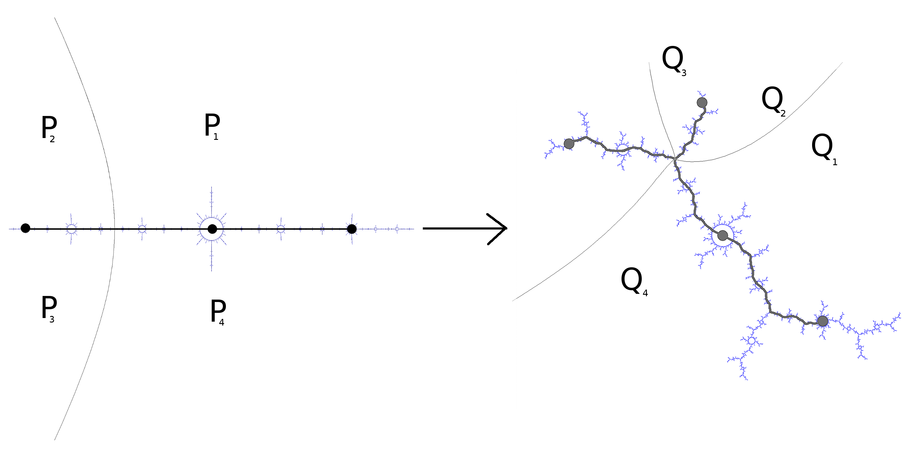
Figure 9. The surgery map $\Psi_{1/3}$. The original tree (left) is a segment, which gets “broken” at the $\alpha$ fixed point and a new branch is added so as to form a tripod (right). External rays belonging to the sectors $P_{1},P_{2},P_{3},P_{4}$ are mapped to sectors $Q_{1},Q_{2},Q_{3},Q_{4}$ respectively.

The image of $1/2$ under $\Psi_{p/q}$ is the external angle of the “tip of the highest antenna” inside the $p/q$-limb and is denoted as $\tau_{p/q}:=\Psi_{p/q}(1/2)=0.\Sigma_{1}$.

Let us now fix a rotation number $p/q$ and denote the surgery map $\Psi_{p/q}$ simply as $\Psi$.

Lemma 14.2.

The map $\Psi$ is strictly increasing (hence injective), in the sense that if $0\leq\theta<\theta^{\prime}<1$, then $0\leq\Psi(\theta)<\Psi(\theta^{\prime})<1$.

Proof.

Let us consider the partitions $P_{1}:=[0,1/3),P_{2}:=[1/3,1/2),P_{3}:=[1/2,2/3)$, $P_{4}:=[2/3,1)$ and $Q_{1}:=[0,0.\overline{0\Sigma_{1}})$, $Q_{2}:=[0.\overline{\Sigma_{0}1},0.\Sigma_{1})$, $Q_{3}:=[0.\Sigma_{1},0.\overline{\Sigma_{1}0})$, $Q_{4}:=[0.\overline{1\Sigma_{0}},1)$. It is elementary (even though a bit tedious) to check that the map $\Psi$ respects the partitions, in the sense that $\Psi(P_{i})\subseteq Q_{i}$ for each $i=1,2,3,4$. Indeed, we know

$$\begin{array}[]{lll}D(P_{1})&\subseteq&P_{1}\cup P_{2}\cup P_{3}\\ D(P_{2})&=&P_{4}\\ D(P_{3})&=&P_{1}\\ D(P_{4})&\subseteq&P_{2}\cup P_{3}\cup P_{4}\end{array}$$

so the binary expansion of any element $\Psi(\theta)$ is represented by an infinite path in the graph

Let us now check for instance that $\Psi(P_{1})\subseteq Q_{1}$. Indeed, if $\theta\in P_{1}$ then in the above graph the coding of $\varphi(\theta)$ starts from $0$ and hence by looking at the graph can be either of the form

$$\Psi(\theta)=0.(0\Sigma_{1})^{k}0^{n}\Sigma_{0}\dots<0.\overline{0\Sigma_{1}}\qquad k\geq 0,n\geq 1$$

or

$$\Psi(\theta)=0.(0\Sigma_{1})^{k}0^{n}\Sigma_{1}\dots<0.\overline{0\Sigma_{1}}\qquad k\geq 0,n\geq 2$$

so in both cases $0\leq\Psi(\theta)<0.\overline{0\Sigma}$ and the claim is proven.

Then, given $0\leq\theta<\theta^{\prime}<1$, let $k$ the smallest integer such that $D^{k}(\theta)$ and $D^{k}(\theta^{\prime})$ lie in two different elements of the partition $\bigcup_{i}P_{i}$. Since the map $D^{k}$ is increasing and the preimage of $0$ lies on the boundary of the partition, we have $D^{k}(\theta)\in P_{i}$ and $D^{k}(\theta^{\prime})\in P_{j}$ with $i<j$, so $\Psi(D^{k}(\theta))<\Psi(D^{k}(\theta^{\prime}))$ because the first one belongs to $Q_{i}$ and the second one to $Q_{j}$, hence we have

$$\Psi(\theta)=0.s_{1}s_{2}\dots s_{k-1}\Psi(D^{k}(\theta))<0.s_{1}s_{2}\dots s_{k-1}\Psi(D^{k}(\theta^{\prime}))=\Psi(\theta^{\prime}).$$

∎

We can also define the map $\Psi$ on the set of real leaves by defining the image of a leaf to be the leaf joining the two images (if $\ell=(\theta_{1},\theta_{2})$, we set $\Psi(\ell):=(\Psi(\theta_{1}),\Psi(\theta_{2}))$). From the previous lemma it follows monotonicity on the set of leaves:

Lemma 14.3.

The surgery map $\Psi=\Psi_{p/q}$ is strictly increasing on the set of leaves. Indeed, if $\{0\}\leq\ell_{1}<\ell_{2}\leq\{1/2\}$, then $\{0\}\leq\Psi(\ell_{1})<\Psi(\ell_{2})\leq\{\tau_{p/q}\}$.

Let us now denote by $\Theta_{0}:=0.\overline{1\Sigma_{0}}$ and $\Theta_{1}:=0.\overline{0\Sigma_{1}}$ the two preimages of $\theta_{0}$ and $\theta_{1}$ which lie in the portrait $C_{p/q}$. Note that $D(\Theta_{i})=\theta_{i}$ for $i=0,1$.

14.3. Forbidden intervals

The leaves $(\theta_{0},\theta_{1})$ and $(\Theta_{0},\Theta_{1})$ divide the circle in three parts. Let us denote by $\Delta_{0}$ the part containing $0$, and as $\Delta_{1}$ the part containing $\tau_{p/q}$. Moreover, for $2\leq i\leq q-1$, let us denote $\Delta_{i}:=D^{i-1}(\Delta_{1})$. With this choice, the intervals $\Delta_{0},\Delta_{1},\dots,\Delta_{q-1}$ are the connected components of the complement of the $\alpha$ portrait $C_{p/q}$.

Let us also denote by $\hat{C}_{p/q}:=C_{p/q}+\frac{1}{2}$ the set of angles of rays landing on the preimage of the $\alpha$ fixed point, and $\hat{\Delta}_{i}:=\Delta_{i}+\frac{1}{2}$ for $0\leq i\leq q-1$, so that $\hat{\Delta}_{0},\hat{\Delta}_{1},\dots,\hat{\Delta}_{q-1}$ are the connected components of the complement of $\hat{C}_{p/q}$.

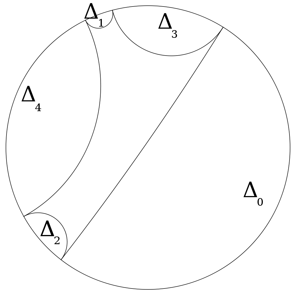
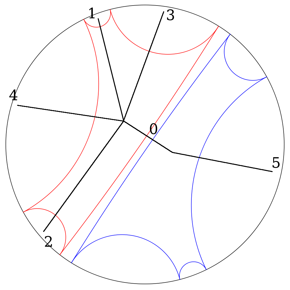
Figure 10. Left: the $\alpha$ fixed portrait $C_{p/q}$ when $p/q=2/5$, with the complementary intervals $\Delta_{i}$. Right: The portraits $C_{p/q}$ and $\hat{C}_{p/q}$, with the Hubbard tree drawn as dual to the lamination. The numbers indicate the position of the iterates of the critical value.

The forbidden interval $I_{p/q}$ is then defined as

$$I_{p/q}:=\bigcup_{i=1}^{q-2}\hat{\Delta}_{i}.$$

The name “forbidden interval” arises from the fact that this interval is avoided by the trajectory of an angle landing on the Hubbard tree of some parameter on the vein $v_{p/q}$. Indeed, the following characterization is true:

Proposition 14.4.

Let $\ell\in P(\tau_{p/q})$ be the characteristic leaf of a parameter $c$ on the principal vein $v_{p/q}$, with $\ell=(\theta^{-},\theta^{+})$, and let $J:=(D^{q-1}(\theta^{-}),D^{q-1}(\theta^{+}))$ the interval delimited by $D^{q-1}(\ell)$ and containing $0$. Then the set of rays landing on the Hubbard tree of $c$ is characterized as

$$H_{c}:=\{\theta\in S^{1}\ :\ D^{n}(\theta)\notin I_{p/q}\cup J\ \ \forall n\geq 0\}.$$

Proof.

It follows from the description of $H_{c}$ in Proposition 8.3 together with the fact that the Hubbard tree is a $q$-pronged star. ∎

The explicit characterization also immediately implies that the sets $H_{c}$ are increasing along principal veins:

Proposition 14.5.

Let $\ell<\ell^{\prime}$ be the characteristic leaves of parameters $c,c^{\prime}$ which belong to the principal vein $v_{p/q}$.

1. Then we have the inclusion

   $$H_{c}\subseteq H_{c^{\prime}};$$

2. if $T_{c}$ and $T_{c^{\prime}}$ are the respective Hubbard trees, we have

   $$h_{top}(f_{c}\mid_{T_{c}})\leq h_{top}(f_{c}\mid_{T_{c^{\prime}}}).$$

Proof.

(1) Let $J$ be the interval containing $0$ delimited by $D^{q-1}(\ell)$, and $J^{\prime}$ the interval delimited by $D^{q-1}(\ell^{\prime})$. Since $\ell<\ell^{\prime}<\{\tau_{p/q}\}$, one has $\{0\}<D^{q-1}(\ell^{\prime})<D^{q-1}(\ell)$, so $J^{\prime}\subseteq J$. If $\theta\in H_{c}$, then by Proposition 14.4 its orbit avoids $I_{p/q}\cup J$, hence it also avoids $I_{p/q}\cup J^{\prime}$ so it must belong to $H_{c^{\prime}}$.

(2) From (1) and Theorem 7.1,

$$h_{top}(f_{c}\mid_{T_{c}})=\textup{H.dim }H_{c}\cdot\log 2\leq\textup{H.dim }H_{c^{\prime}}\cdot\log 2=h_{top}(f_{c^{\prime}}\mid_{T_{c^{\prime}}}).$$

∎

Monotonicity of entropy along arbitrary veins is proven, for postcritically finite parameters, in Tao Li’s thesis [TaoL]. Recently, the following very elegant argument, proving monotonicity along veins without the restriction to postcritically finite parameters, was suggested by Tan Lei.

Proposition 14.6.

Let $\ell<\ell^{\prime}$ be the characteristic leaves of $c,c^{\prime}$, with $\ell^{\prime}$ non-degenerate. Then the entropies of the respective Hubbard trees satisfy the inequality

$$h_{top}(f_{c}\mid_{T_{c}})\leq h_{top}(f_{c^{\prime}}\mid_{T_{c^{\prime}}}).$$

Proof.

Fix $\ell=(\theta^{-},\theta^{+})$ a leaf of $QML$, and consider the sets

$$U_{1}:=\left(\frac{\theta^{+}}{2},1+\frac{\theta^{-}}{2}\right)$$

$$U_{2}:=\left(1+\frac{\theta^{+}}{2},\frac{\theta^{-}}{2}\right).$$

Define the set $\Sigma(\ell)$ to be the set of angle pairs whose forward orbit never lies outside $U_{1}\cup U_{2}$, and which always have the same itinerary with respect to the partition $U_{1}\cup U_{2}$:

$$\begin{array}[]{ll}\Sigma(\ell):=\{(\xi,\eta)\in S^{1}\times S^{1}\ :\ \xi\neq\eta,\ \forall n\geq 0&D^{n}(\eta)\in U_{1}\cup U_{2},\\ &D^{n}(\xi)\in U_{1}\cup U_{2},\\ &D^{n}(\xi)\in U_{i}\Leftrightarrow D^{n}(\eta)\in U_{i}\}.\\ \end{array}$$

and denote $U(\ell):=\{\theta\in S^{1}\ :\exists\eta\in S^{1}\textup{ s.t. }(\theta,\eta)\in\Sigma(\ell)\}$ the set of endpoints of angle pairs in $\Sigma(\ell)$. Since the intervals $(\theta^{-}/2,\theta^{+}/2)$ and $(1+\theta^{-}/2,1+\theta^{+}/2)$ do not contain rays landing on the Hubbard tree, then we have (up to a countable set of angles which hit the boundary of the partition) the inclusion

$$H_{c}\subseteq U(\ell).$$

On the other hand, the two elements of an angle pair $(\xi,\eta)$ which belongs to $\Sigma(\ell)$ have the same itinerary with respect to the partition $(\theta^{-}/2,1+\theta^{-}/2)\cup(1+\theta^{-}/2,\theta^{-}/2)$, so the rays at angles $\xi$ and $\eta$ must land at the same point, which is then biaccessible. This proves the inclusion

$$U(\ell)\subseteq B_{c},$$

which combined with the previous one implies that $\textup{H.dim }H_{c}=\textup{H.dim }U(\ell)$. Now, from the definition it is clear that if $\ell<\ell^{\prime}$ then $\Sigma(\ell)\subseteq\Sigma(\ell^{\prime})$, since the sets $U_{1}$ and $U_{2}$ become larger as $\ell$ gets larger. Hence we have $U(\ell)\subseteq U(\ell^{\prime})$ and $\textup{H.dim }H_{c}\leq\textup{H.dim }H_{c^{\prime}}$, which proves the claim.

∎

14.4. Surgery in the dynamical and parameter planes

The usefulness of the surgery map comes from the fact that it maps the real vein in parameter space to the other principal veins, and also the Hubbard trees of parameters along the real vein to Hubbard trees along the principal veins. As we will see in this subsection, the correspondence is almost bijective.

Let $Z$ denote the set of angles which never map to the endpoints of fixed leaf $\ell_{0}=(1/3,2/3)$:

$$Z:=\{\theta\in S^{1}\ :\ D^{n}(\theta)\neq 1/3,2/3\ \ \forall n\geq 0\}.$$

Moreover, we denote by $\Omega$ the set of angles which never map to either the forbidden interval $I_{p/q}$ or the $\alpha$ portrait $C_{p/q}$:

$$\Omega:=\{\theta\in\Delta_{0}\cup\Delta_{1}\ :\ D^{n}(\theta)\notin I_{p/q}\cup C_{p/q}\ \ \forall n\geq 0\}.$$

It is easy to check the following

Lemma 14.7.

The map $\Psi$ is continuous on $Z$, and the image $\Psi(Z)$ is contained in $\Omega$. Given $\theta\in\Omega$, let $0=n_{0}<n_{1}<n_{2}<\dots$ be the return times of $\theta$ to $\Delta_{0}\cup\Delta_{1}$. Then the map

$$\Phi(\theta):=0.s_{0}s_{1}s_{2}\dots\qquad\textup{with }s_{k}=\left\{\begin{array}[]{ll}0&\textup{if }D^{n_{k}}(\theta)\in[0,\Theta_{1})\cup(\theta_{0},\tau_{p/q})\\ 1&\textup{if }D^{n_{k}}(\theta)\in[\tau_{p/q},\theta_{1})\cup(\Theta_{0},1)\end{array}\right.$$

defined on $\Omega$ is an inverse of $\Psi$, in the sense that $\Phi\circ\Psi(\theta)=\theta$ for all $\theta\in Z$.

Proposition 14.8.

The surgery map $\Psi=\Psi_{p/q}$ maps the real combinatorial vein bijectively onto the principal combinatorial vein $P(\tau_{p/q})$ in the $p/q$-limb, up to a countable set of prefixed parameters; indeed, one has the inclusions

$$P(\tau_{p/q})\setminus\bigcup_{n\geq 0}D^{-n}(C_{p/q})\subseteq\Psi(P(1/2))\subseteq P(\tau_{p/q}).$$

Proof.

Let $m\in P(1/2)$ be a minor leaf, and $M_{1}$, $M_{2}$ its major leaves. By the criterion of Proposition 3.3, all the elements of the forward orbit of $m$ have disjoint interior, and their interior is also disjoint from $m$, $M_{1}$ and $M_{2}$, so the set of leaves $\{D^{n}(m)\ :\ n\geq 0\}\cup\{M_{1},M_{2}\}$ (which may be finite or infinite) is totally ordered, and they all lie between $\{0\}$ and $\{1/2\}$. Indeed, they are all smaller than $m$, which is also the shortest leaf of the set. Now, by Lemma 14.3, the set

$$\{\Psi(D^{n}(m))\ :\ n\geq 0\}\cup\{\Psi(M_{1}),\Psi(M_{2})\}$$

is also totally ordered, and all its elements have disjoint interior and lie between $\{0\}$ and $\Psi(m)$. Note that all leaves smaller than $\ell_{0}:=(1/3,2/3)$ map under $\Psi$ to leaves smaller than $(\Theta_{0},\Theta_{1})$, and all leaves larger than $\ell_{0}$ map to leaves larger than $\Psi(\ell_{0})=(\theta_{0},\theta_{1})$. Note moreover that if a leaf $\mathcal{L}$ is larger than $(\theta_{0},\theta_{1})$, then its length increases under the first $q-1$ iterates (i.e. until it comes back to $\Delta_{0}$):

$$\ell(D^{k}(\mathcal{L}))=2^{k}\ell(\mathcal{L})\qquad 0\leq k\leq q-1.$$

As a consequence, the shortest leaf in the set

$$S:=\{D^{n}(\Psi(m))\ :\ n\geq 0\}\cup\{\Psi(M_{1}),\Psi(M_{2})\}$$

is $\Psi(m)$, and its images all have disjoint interiors, hence by Proposition 3.3 we have that $\Psi(m)$ belongs to $QML$, and it is smaller than $\tau_{p/q}$ by monotonicity of $\Psi$. Conversely, any leaf $\ell$ of $P(\tau_{p/q})$ whose endpoints never map to the fixed orbit portrait $C_{p/q}$ belongs to $\Omega$, hence $\Psi(\ell)$ is well-defined and, since $\Psi$ preserves the ordering, it belongs to $P(1/2)$ by Proposition 3.3. ∎

Proposition 14.9.

Let $c\in[-2,1/4]$ be a real parameter, with characteristic leaf $\ell$, and let $c^{\prime}$ be a parameter with characteristic leaf $\ell^{\prime}=\Psi(\ell)$. Moreover, let us set $\tilde{H}_{c^{\prime}}:=H_{c^{\prime}}\cap(\Delta_{0}\cup\Delta_{1})\setminus\bigcup_{n}D^{-n}(C_{p/q})$. Then the inclusions

$$\tilde{H}_{c^{\prime}}\subseteq\Psi(H_{c})\subseteq H_{c^{\prime}}$$

hold. As a consequence,

$$\textup{H.dim }\Psi(H_{c})=\textup{H.dim }H_{c^{\prime}}.$$

Proof.

Let $\theta\in H_{c}$ and $\ell:=(\theta,1-\theta)$ be its associated real leaf and let $\ell_{c}$ the postcharacteristic leaf for $f_{c}$. Let us first assume $D^{n}(\theta)\neq 1/3,2/3$ for all $n$. Then by Lemma 14.7 $\Psi(\theta)$ lies in $\Omega$, so its orbit always avoids $I_{p/q}$. Moreover, by Proposition 8.3

$$D^{n}(\ell)\geq\ell_{c}\qquad\textup{for all }n\geq 0.$$

Then, by monotonicity of the surgery map (Lemma 14.3)

$$\Psi(D^{n}(\ell))\geq\Psi(\ell_{c})\qquad\textup{for all }n\geq 0.$$

Moreover, given $N\geq 0$ either

$$D^{N}(\Psi(\ell))\notin\Delta_{0}\cup\Delta_{1}$$

or one can write

$$D^{N}(\Psi(\ell))=\Psi(D^{n}(\ell))$$

for some integer $n$, so the orbit of $\Psi(\theta)$ always avoids the interval delimited by the leaf $\Psi(\ell_{c})$, hence by Proposition 8.3 we have $\Psi(\theta)\in H_{c^{\prime}}$. The case when $D^{n}(\theta)$ hits $\{1/3,2/3\}$ is analogous, except that the leaf $\ell$ is eventually mapped to the leaf $(\theta_{0},\theta_{1})$ which belongs to the $\alpha$ portrait.

Conversely, let $\theta^{\prime}\in\tilde{H}_{c^{\prime}}$ and $\ell^{\prime}$ be its corresponding leaf. Then by Proposition 14.4 it never maps to $I_{p/q}$, so by Lemma 14.7 there exists $\theta\in Z$ such that $\theta^{\prime}=\Psi(\theta)$. Let $\ell:=(\theta,1-\theta)$ be its corresponding real leaf. Moreover, also by Proposition 14.4 all iterates of $\ell^{\prime}$ are larger than $\Psi(\ell_{c})$, so by monotonicity of the surgery map all iterates of $\ell$ are larger than $\ell_{c}$, so, by Proposition 8.3, $\theta$ lies in $H_{c}$. The equality of dimensions arises from the fact that for $2\leq i\leq q-1$ one has

$$H_{c^{\prime}}\cap\Delta_{i}=D^{q-1}(H_{c^{\prime}}\cap\Delta_{1})$$

and the doubling map preserves Hausdorff dimension. ∎

Finally, we need to check that the surgery map behaves well under renormalization. Indeed we have the

Lemma 14.10.

Let $W$ be a real hyperbolic component, and $\Psi$ the surgery map. Then for each $\theta\in\mathcal{R}$,

$$\Psi(\tau_{W}(\theta))=\tau_{\Psi(W)}(\theta)$$

where $\Psi(W)$ is the hyperbolic component whose endpoints are the images via surgery of the endpoints of $W$.

Proof.

Let $\theta=0.\theta_{1}\theta_{2}\dots$ be the binary expansion of $\theta$. Denote as $\theta^{-}=0.\overline{S_{0}}$, $\theta^{+}=0.\overline{S_{1}}$ the angles of parameter rays landing at the root of $W$, and as $\Theta^{-}:=\Psi(\theta^{-})=0.\overline{T_{0}}$ and $\Theta^{+}:=\Psi(\theta^{+})=0.\overline{T_{1}}$ the angles landing at the root of $\Psi(W)$. Finally, let $p:=|S_{0}|$ denote the the period of $W$. Then $\tau_{W}(\theta)$ has binary expansion

$$\tau_{W}(\theta)=0.S_{\theta_{1}}S_{\theta_{2}}\dots$$

By using the fact that either $\theta^{-}\leq\theta^{+}<1/3$ or $2/3<\theta^{-}\leq\theta^{+}$, one checks that for each $0\leq k<p$, the points

$$D^{k}(0.S_{\theta_{1}}S_{\theta_{2}}\dots)$$

and

$$D^{k}(0.\overline{S_{\theta_{1}}})$$

lie in the same element of the partition $\bigcup_{i=1}^{4}P_{i}$. As a consequence, by definition of the surgery map $\Psi$, we get that

$$\Psi(\tau_{W}(\theta))=0.T_{\theta_{1}}T_{\theta_{2}}\dots$$

and the claim follows.

∎

14.5. Proof of Theorem 1.3

Definition 14.11.

The set $\mathcal{D}_{p/q}$ of dominant parameters along $v_{p/q}$ is the image of the set of (real) dominant parameters $\mathcal{D}$ under the surgery map:

$$\mathcal{D}_{p/q}:=\Psi_{p/q}(\mathcal{D}).$$

We can now use the surgery map to transfer the inclusion of the Hubbard trees of real maps in the real slice of the Mandelbrot set to an inclusion of the Hubbard trees in the set of angles landing on the vein in parameter space.

Proposition 14.12.

Let $c\in v_{p/q}$ be a parameter along the vein with non-renormalizable combinatorics, and $c^{\prime}$ another parameter along the vein which separates $c$ from the main cardioid (i.e. if $\ell$ and $\ell^{\prime}$ are the characteristic leaves, $\ell^{\prime}<\ell\leq\{\tau_{p/q}\}$). Then there exists a piecewise linear map $F:\mathbb{R}/\mathbb{Z}\to\mathbb{R}/\mathbb{Z}$ such that

$$F(\tilde{H}_{c^{\prime}})\subseteq P_{c}.$$

Proof.

Let $\theta\in[0,\tau_{p/q}]$ be a characteristic angle for $c$. Let us first assume that the forward orbit of $\theta$ never hits $C_{p/q}$. Then by Proposition 14.8 there exists an angle $\theta_{R}\in[0,1/2]\cap\mathcal{R}$ such that $\theta=\Psi(\theta_{R})$, and by Lemma 14.10 $\theta_{R}$ is not renormalizable. Then, by Proposition 10.1, there exist a $\theta^{\prime}_{R}<\theta_{R}$ arbitrarily close to $\theta_{R}$ (and by continuity of $\Psi$ we can choose it so that $\Psi(\theta^{\prime}_{R})$ lands on the vein closer to $c$ than $c^{\prime}$) and a piecewise linear map $F_{R}$ of the circle such that

(10) $$F_{R}(H_{\theta^{\prime}_{R}})\subseteq P_{\theta_{R}}.$$

We claim that the map $F:=\Psi\circ F_{R}\circ\Psi^{-1}$ satisfies the claim. Indeed, if $\xi\in[0,1/2)$ recall that the map $F_{R}$ constructed in Proposition 10.1 has the form

$$F_{R}(\xi)=s+\xi\cdot 2^{-N}$$

where $s$ is a dyadic rational number and $N$ is some positive integer. Thus, $D^{N}(F_{R}(\xi))=\xi$, so also

$$\Psi(\xi)=\Psi(D^{N}(F_{R}(\xi)))=D^{M}(\Psi(F_{R}(\xi)))$$

for some integer $M$. Thus we can write for $\xi\in H_{\theta^{\prime}_{R}}\cap Z$

$$\Psi(F_{R}(\xi))=t+\Psi(\xi)\cdot 2^{-M}$$

where $t$ is a dyadic rational number, and $t$ and $M$ only depend on $s$ and the element of the partition $\bigcup P_{i}$ to which $\xi$ belongs. Thus we have proven that $F=\Psi\circ F_{R}\circ\Psi^{-1}$ is piecewise linear. Now, by Proposition 14.9, eq. (10), and Proposition 14.8 we have the chain of inclusions

$$\Psi\circ F_{R}\circ\Psi^{-1}(\tilde{H}_{c^{\prime}})\subseteq\Psi\circ F_{R}(H_{\theta^{\prime}_{R}})\subseteq\Psi(P_{\theta_{R}})\subseteq P_{c}.$$

Finally, if the forward orbit of $\theta$ hits $C_{p/q}$, then by density one can find an angle $\tilde{\theta}\in(\theta^{\prime},\theta)$ such that its forward orbit does not hit $C_{p/q}$, and apply the previous argument to the parameter $\tilde{c}$ with characteristic angle $\tilde{\theta}$, thus getting the inclusion

$$F(\tilde{H}_{c^{\prime}})\subseteq P_{\tilde{c}}\subseteq P_{c}.$$

∎

Proof of Theorem 1.3..

Let $c$ be a parameter along the vein $v_{p/q}$. Then by Theorem 5.5

$$\frac{h_{top}(f_{c}\mid_{T_{c}})}{\log 2}=\textup{H.dim }H_{c}.$$

We shall prove that the right hand side equals $\textup{H.dim }P_{c}$. Now, since $P_{c}\subseteq H_{c}$, it is immediate that

$$\textup{H.dim }P_{c}\leq\textup{H.dim }H_{c}$$

hence we just have to prove the converse inequality. Let us now assume $c\in v_{p/q}$ non-renormalizable. Then by Proposition 14.12 for each $c^{\prime}\in[0,c]$ we have the inclusion

$$F(\tilde{H}_{c^{\prime}})\subseteq P_{c}$$

so, since $F$ is linear hence it preserves Hausdorff dimension, we have

$$\textup{H.dim }H_{c^{\prime}}=\textup{H.dim }\tilde{H}_{c^{\prime}}\leq\textup{H.dim }P_{c}$$

and as a consequence

$$\textup{H.dim }P_{c}\geq\sup_{c^{\prime}\in[0,c]}\textup{H.dim }H_{c^{\prime}}$$

where $[0,c]$ is the segment of the vein $v_{p/q}$ joining $0$ with $c$. Now by continuity of entropy (Theorem 13.5)

$$\sup_{c^{\prime}\in[0,c]}\textup{H.dim }H_{c^{\prime}}=\textup{H.dim }H_{c}$$

hence the claim is proven for all non-renormalizable parameters along the vein. Now, the general case follows as in the proof of Theorem 1.7 by successively renormalizing and using the formulas of Proposition 11.2. ∎

So far we have worked with the combinatorial model for the veins, which conjecturally coincide with the set of angles of rays which actually land on the vein. Finally, the following proposition proves that the vein and its combinatorial model actually have the same dimension, independently of the MLC conjecture.

Proposition 14.13.

Let $c\in v_{p/q}\cap\partial\mathcal{M}$ and $\ell$ its characteristic leaf. Let

$$\overline{P}_{c}:=\{\theta\in S^{1}\ :\ R_{M}(\theta)\textup{ lands on }v\cap[0,c]\}$$

be the set of angles of rays landing on the vein $v$ closer than $c$ to the main cardioid, and

$$P_{c}:=\{\theta\in S^{1}\ :\ \theta\textup{ is endpoint of some }\ell^{\prime}\in QML,\ \ell^{\prime}\leq\ell\}$$

its combinatorial model. Then the two sets have equal dimension:

$$\textup{H.dim }\overline{P}_{c}=\textup{H.dim }P_{c}.$$

Proof.

Fix a principal vein $v_{p/q}$, and let $\tau_{W}$ be the tuning operator relative to the hyperbolic component of period $q$ in $v_{p/q}$; moreover, denote as $\tau$ the tuning operator relative to the hyperbolic component of period $2$. Let $P_{c}^{fr}$ the set of angles which belong to the $P_{c}$ with finitely renormalizable combinatorics; then Proposition 3.2 yields the inclusions

$$\textup{H.dim }P_{c}^{fr}\subseteq\textup{H.dim }\overline{P}_{c}\subseteq\textup{H.dim }P_{c}$$

hence to prove the proposition it is sufficient to prove the equality

$$\textup{H.dim }P_{c}^{fr}=\textup{H.dim }P_{c}.$$

Let now $c_{n}:=\tau_{W}(\tau^{n}(-2))$ the tips of the chain of nested baby Mandelbrot sets which converge to the Feigenbaum parameter in the $p/q$-limb, and let $\ell_{n}$ be the characteristic leaf of $c_{n}$. Then if $\textup{H.dim }P_{c}>0$, there exists a unique $n\geq 1$ such that $\ell_{n}<\ell\leq\ell_{n-1}$, hence by monotonicity and by Theorem 1.3 we know

$$\textup{H.dim }P_{c}\geq\textup{H.dim }P_{c_{n}}=\frac{1}{2^{n}q}.$$

Now, each element of $P_{c}$ is either of the form $\tau_{W}\tau^{n-1}(c^{\prime})$ with $c^{\prime}$ non-renormalizable, or of the form $\tau_{W}(\tau^{n-1}(\tau_{V}(c^{\prime})))$ where $V$ is some hyperbolic window of period larger than $2$. However, we know by Proposition 11.2 that the image of $\tau_{W}\circ\tau^{n-1}\circ\tau_{V}$ has Hausdorff dimension at most $\frac{1}{q\cdot 2^{n-1}\cdot 3}<\textup{H.dim }P_{c}$, hence one must have

$$\textup{H.dim }P_{c}=\textup{H.dim }\{\theta\in\overline{P}_{c}\ :\ \theta=\tau_{W}\tau^{n-1}(\theta^{\prime}),\ \theta^{\prime}\textup{ non-renormalizable}\}\leq\textup{H.dim }P_{c}^{fr}$$

which yields the claim. ∎

References

- [BdC] M. Baillif, A. de Carvalho, Piecewise linear model for tree maps, Internat. J. Bifur. Chaos Appl. Sci. Engrg. 11 (2001), no. 12, 3163–3169.
- [Bi] P. Billingsley, Ergodic theory and information, John Wiley & Sons Inc., New York, 1965, xiii+195.
- [BCIT] C. Bonanno, C. Carminati, S. Isola, G. Tiozzo, Dynamics of continued fractions and kneading sequences of unimodal maps, Discrete Contin. Dyn. Syst. 33 (2013), no. 4, 1313–1332.
- [Bo] R. Bowen, Entropy for group endomorphisms and homogeneous spaces, Trans. Amer. Math. Soc. 153 (1971), 401–414.
- [BD] B. Branner, A. Douady, Surgery on complex polynomials, Holomorphic dynamics (Mexico, 1986), Lecture Notes in Math. 1345, 11–72, Springer, Berlin, 1988.
- [BS] H. Bruin, D. Schleicher, Hausdorff dimension of biaccessible angles for quadratic polynomials, preprint arXiv:1205.2544.
- [CT] C. Carminati, G. Tiozzo, A canonical thickening of and the entropy of -continued fraction transformations, Ergodic Theory Dynam. Systems 32 (2012), no. 4, 1249–1269.
- [CT2] C. Carminati, G. Tiozzo, The bifurcation locus for numbers of bounded type, arxiv:1109.0516.
- [CFS] I. P. Cornfeld, S. V. Fomin, and Ya. G. Sinaĭ, Ergodic theory, Grundlehren der Mathematischen Wissenschaften [Fundamental Principles of Mathematical Sciences] 245, Springer-Verlag, New York, 1982.
- [dMvS] W. de Melo and S. van Strien, “One-dimensional Dynamics,” Springer-Verlag, Berlin, Heidelberg, 1993.
- [Do1] A. Douady, Algorithms for computing angles in the Mandelbrot set, in Chaotic dynamics and fractals (Atlanta, Ga., 1985), Notes Rep. Math. Sci. Engrg. 2, 155–168, Academic Press, Orlando, 1986.
- [Do2] A. Douady, Descriptions of compact sets in , in Topological methods in modern mathematics (Stony Brook, NY, 1991), 429–465, Publish or Perish, Houston, 1993.
- [Do3] A. Douady, Topological entropy of unimodal maps: monotonicity for quadratic polynomials, in Real and complex dynamical systems (Hillerød, 1993), NATO Adv. Sci. Inst. Ser. C Math. Phys. Sci. 464, 65–87, Kluwer, Dordrecht, 1995.
- [DH] A. Douady, J. H. Hubbard, On the dynamics of polynomial-like mappings, Ann. Sci. École Norm. Sup. (4), 18, (1985), no. 2, 287–343.
- [DH2] A. Douady, J. H. Hubbard, Étude dynamique des polynômes complexes, Publications Mathématiques d’Orsay 84, Université de Paris-Sud, Département de Mathématiques, Orsay, 1984.
- [Fa] K. Falconer, Fractal geometry: mathematical foundations and applications, Wiley, Chichester, 1990.
- [Fu] H. Furstenberg, Disjointness in ergodic theory, minimal sets, and a problem in Diophantine approximation, Math. Systems Theory 1 (1967), 1–49.
- [Hu] J. H. Hubbard, Local connectivity of Julia sets and bifurcation loci: three theorems of J.-C. Yoccoz, in Topological methods in modern mathematics (Stony Brook, NY, 1991), 467–511, Publish or Perish, Houston, 1993.
- [LeYo] F. Ledrappier, L.-S. Young, The metric entropy of diffeomorphisms. II. Relations between entropy, exponents and dimension, Ann. of Math. (2) 122 (1985), no. 3, 540–574.
- [LvS] G. Levin, S. van Strien, Local connectivity of the Julia set of real polynomials, Ann. of Math. (2) 147 (1998), no. 3, 471–541.
- [Ly] M. Yu. Lyubich, Entropy of analytic endomorphisms of the Riemann sphere, Funktsional. Anal. i Prilozhen. 15 (1981), no. 4, 83–84, translated in Functional Anal. Appl. 15 (1981), no. 4, 300–302.
- [Ly2] M. Yu. Lyubich, Feigenbaum-Coullet-Tresser universality and Milnor’s hairiness conjecture, Ann. of Math. (2) 149 (1999), no. 2, 319–420.
- [Ma] A. Manning, A relation between Lyapunov exponents, Hausdorff dimension and entropy, Ergodic Theory Dynam. Systems 1 (1981), no. 4, 451–459.
- [Mc] C. T. McMullen, Complex dynamics and renormalization, Annals of Mathematics Studies 135, Princeton University Press, Princeton, NJ, 1994.
- [Mi1] J. Milnor, Periodic orbits, external rays and the Mandelbrot set: an expository account, Astérisque 261 (2000), 277-333.
- [Mi2] J. Milnor, Local connectivity of Julia sets: expository lectures, in The Mandelbrot set, theme and variations, London Math. Soc. Lecture Note Ser. 274, 67–116, Cambridge Univ. Press, Cambridge, 2000.
- [MT] J. Milnor, W. Thurston, On iterated maps of the interval, Dynamical systems (College Park, MD, 1986–87), Lecture Notes in Math., 1342, 465–563, Springer, Berlin, 1988.
- [MS] M. Misiurewicz, W. Szlenk, Entropy of piecewise monotone mappings, Studia Math. 67 (1980), no. 1, 45–63.
- [Po] C. Pommerenke, Boundary behaviour of conformal maps, Grundlehren der Mathematischen Wissenschaften 299, Springer-Verlag, Berlin, 1992.
- [Ri] J. Riedl, Arcs in Multibrot Sets, Locally Connected Julia Sets and Their Construction by Quasiconformal Surgery, PhD Thesis, TU München, 2001.
- [Sch] D. Schleicher, On Fibers and Renormalization of Julia Sets and Multibrot Sets, Stony Brook IMS preprint 1998/13b, available on arXiv:math/9902156 [math.DS].
- [Sm] S. Smirnov, On supports of dynamical laminations and biaccessible points in polynomial Julia sets, Colloq. Math. 87, (2001), 2, 287–295.
- [Th1] W. Thurston, On the Geometry and Dynamics of Iterated Rational Maps, in D Schleicher, N Selinger, editors, “Complex dynamics”, 3–137, A K Peters, Wellesley, MA, 2009.
- [Th2] W. Thurston, Entropy in dimension one, preprint 2011.
- [TanL] Tan Lei, Similarity between the Mandelbrot set and the Julia sets, Commun. Math. Phys. 134 (1990), 587–617.
- [TaoL] Tao Li, A monotonicity conjecture for the entropy of Hubbard trees, PhD Thesis, SUNY Stony Brook, 2007.
- [Wi] S. Willard, General topology, Addison-Wesley Publishing Co., Reading, Mass.-London-Don Mills, Ont., 1970.
- [Yo] L.-S. Young, Dimension, entropy and Lyapunov exponents, Ergodic Theory Dynam. Systems 2 (1982), no. 1, 109–124.
- [Za1] S. Zakeri, Biaccessibility in quadratic Julia sets, Ergodic Th. Dyn. Sys. 20 no. 6 (2000), 1859–1883.
- [Za] S. Zakeri, External Rays and the Real Slice of the Mandelbrot Set, Ergod. Th. Dyn. Sys. 23 (2003), 637–660.
- [Za2] S. Zakeri, On biaccessible points of the Mandelbrot set, Proc. Amer. Math. Soc. 134 (2006), no. 8, 2239–2250.
- [Zd] A. Zdunik, On biaccessible points in Julia sets of polynomials, Fund. Math. 163 (2000), no. 3, 277–286.