More on Superconductors via Gauge/Gravity Duality with Nonlinear Maxwell Field

Abstract

We have developed the recent investigations on the second-order phase transition in the holographic superconductor using the probe limit for a nonlinearMaxwell field strength coupled to amassless scalar field. By analytical methods, based on the variational Sturm-Liouville minimization technique, we study the effects of the spacetime dimension and the nonlinearity parameter on the critical temperature and the scalar condensation of the dual operators on the boundary. Further, as a motivated result, we analytically deduce theDCconductivity in the lowand zero temperatures regime. Especially in the zero temperature limit and in two dimensional toy model, we thoroughly compute the conductivity analytically. Our work clarifies more features of the holographic superconductors both in different space dimensions and on the effect of the nonlinearity in Maxwell’s strength field.

I Introduction

In the recent years, using the holographic picture of the world, the AdS/CFT (anti de Sitter/conformal field theory) correspondence [1-3] has been applied to study some strongly correlated systems in condensed matter physics, especially for strongly coupled systems with the scaleinvariance. Particularly, people studied the low temperature, quantum critical systems near critical point (see, e.g., [4, 5] and references therein). The critical phenomena, which happen here, is a second-order phase transition from normal phase to the superconducting phase, in which below a specific temperature 𝑇 𝑐, the DC conductivity becomes infinite. Such second-order phase transitions happen in the high-temperature superconductors and can be described very well by the AdS/CFT dictionary [6, 7]. From the classical and phenomenological point of view, superconductivity, in the high-temperature type II superconductors,formulated using a phenomenological based Landau-Ginzburg Lagrangian. This Lagrangian contains a general complex value scalar field Ψ, plays the role of a condensate in a superconductive phase. Basically, to have a scalar condensation in the boundary quantumfield theory using CFT on the boundary of the bulk,Hartnoll et al [8] proposed a Lagrangian of an abelian gauge field 𝐴 𝜇and a complex scalar field with mass above the Breitenlohner-Freedman (BF) bound [9]. Later Gubser [10] stdied the hairy black holes and he showed that how the dual operators has the same temperature dependence as the condensation in superconductors.

The full description of the superconductivity in the probe limit or away this limit needs to provide the numerical solutions of a couple of nonlinear differential equations. By simplicity, they can be solved using the shooting approach by expanding in series the functions and matching these by varying the free parameters of the series in a typical point between the horizon and the spatial infinity. Parallel to the numerical studies, recently some analytical approaches have been proposed to find the universal properties of secondorder phase transitions in holographic superconductors [11– 18]. In particular, the authors in [18] used the variational functional method. In [18, 19] this analytical method has been used to calculate critical properties like temperature and critical exponent. The eigenvalue of this variational problem is a function of the critical chemical potential 𝜇 𝑐$\mu_{c}$, and consequently, it is related to the 𝑇 𝑐$T_{c}$. another types of super criticality have been studied depending on the dual operators on boundary [20]. Also, one can apply this method to superconductors with external magnetic fields[21, 22]. Furthermore, a number of aspects of external and bulk magnetic fields in holographic superconductors have been investigated [23-26]. The phase transition can be interpreted in terms of the string interactions [27-31]. The effects of the nonlinear electrodynamics in the holographic superconductors have been investigated recently [32-36]. There are many interests in the modified gravity theories. For example, on Gauss-Bonnet and Weyl corrected superconductors, on which, we are working with a higher derivative corrected bulk black hole, like Weyl corrections [37] numerically. Furthermore, we have studied the Weyl corrections to the superconductors analytically [38, 39]. Moreover, we showed that there exists a family of p-wave holographic withWeyl corrections [40]. In the present paper, we would like to study the $((𝑑d-2)+1)$-dimensional holographic superconductor in the probe limit for a power law Maxwell field strength $(F^{\mu\nu}F_{\mu\nu})^{\delta}$ coupled to a scalar field. We focus just on the s-wave cases. We must clarify the motivation of the s-wave approximation in holographic models of superconductors. In the relativistic models of the gravity, it is highly known that s-wave approximation is not a good approximation, for example, in the cosmological models and black holes [41]. The meaning of the s-wave here does not back to the reduction of the action from four to two dimensional like the dilatonic action from the four dimensional spinor (Majorana) action. We mean by s-wave, in the context of holographic superconductors, a scalar order parameter, whose expectation value breaks the U(1) but not rotational symmetry.Moreover, we can have the Yang-Mills fields with 𝑆𝑈(2) symmetry which additionally they can generate another symmetry breaking of an axial vector type. The last case resembles the p-wave models. We mention here that the three dimensional non-linear model of the superconductors,which we used in this paper, is a realistic model and it will be more interesting that we can find a direct relation between this nonlinear model and the results of a higher dimensional model, by a principle like the detailed balance. Another additional point is to restrict ourselves just to the case of a single horizon. The problem of the multihorizon cases needs more investigation, for example, the case of the Nariai black holes. The theory here will be so different. This later appeared in the lower dimensional models. For example, the case of the quantum corrected BTZ like black hole is a good example [42]. In the holographic set up for superconductors one must identify a temperature in his gravitational bulk model to the CFT temperature on the boundary. If the black hole has only one horizon, in this case, we can use the Hawking-Bekenstein (horizon) or Kodama- Hayward temperature [43] as a reasonable candidate. But if our asymptotically AdS bulk has more than one horizon, for example, in the case of the charged BTZ like black holes, then we take the temperature of the real physical horizon (the temperature which is obtained by calculation the surface gravity of the biggest null hypersurface orthogonal surface) as the candidate for temperature of the CFT. In fact the effects of the quantum corrections and chargedMaxwell field on the background of the bulk are very interesting problems and can be investigated in more details. Also it is possible to relate the instability of such charged dilaton configurations in the AdS spacetime [44] to the symmetry breaking mechanism of the superconductors.The idea has motivation enough as a new work. In this paper we investigate analytically the effect of the spacetime dimension 𝑑 and the power $\delta$ on the critical temperature 𝑇 𝑐. Although our problem is the especial massless case of the model which has been investigated recently [45],49 , we study these corrections to the superconductors analytically. Additionally, we want to compute the DC conductivity for this kind of the superconductor using the perturbation method. In this approach, we apply an external linear electromagnetic field. This field is periodic in time. By calculating, the response in the first order linear approximation, we compute the conductivity for the low temperature case, especially for zero temperature configuration. Our plan in this paper is as the following. In Section 2, we clarify our motivation for considering the nonlinearMaxwell action instead of the linear theory. In Section 3, introduce ourmodel for holographic superconductors. In Section 4, we apply the variational method to obtain the critical temperature of the system. In Section 5, we calculate the critical exponent for the condensation operator. In Sections 6 and 7 we compute the conductivity for low and zero temperature cases.We summarize and conclude in the final section.

II Motivation for nonlinear Maxwell effects in holographic superconductors

Thelinear approximations in themathematical physics, as we know, have limitations, both in predictions of the model and especially on matching with the full description of the model using the numerical results.The linearMaxwell theory fails in some domains, and it is needed to consider the general form of the Lagrangian instead of the linear one. The Lagrangian of the Maxwell model is:

$$\mathcal{L}_{M}=-\frac{1}{4}F^{2},$$ (1)

where $F^{2}=F^{\mu\nu}F_{\mu\nu}$. A natural extension of (1) is obtained by replacing a general function of 𝐹 in the form $\Phi(F)$. Recently, it has been shown that such nonlinear general forms have a rich family of black holes in $f(R)$ gravity [46]. There are different reasons for investigating these forms. The oldest one may be the Born-Infeld (BI) alternative for linear Maxwell’s theory.In string theory language, this BI action can be replaced by the tachyonic action. The BI Lagrangian reads [47]:

$$\mathcal{L}_{BI}=\eta^{2}(1-\sqrt{1+\frac{F^{2}}{2\eta^{2}}}).$$ (2)

Here $\eta$ is the string’s tension parameter. This form reduces to the (1) in the limit of $\eta\rightarrow\infty$. Indeed, we can expand in series (2) in the following form:

$$\mathcal{L}_{BI}=\sum_{n=1}^{\infty}c_{n}\eta^{2(1-n)}F^{2n}.$$ (3)

The leading order term $n=1$ is just in form of (1). Even, if we don’t work with BI theory, this nonlinearity meets us from a geometrical point of view. Suppose that we want to write a conformal invariance (CI) Lagrangian, constructed from the $U(1)$ gauge fields $A^{\mu}$. Such CI is the invariance of the whole theory under geometrical transformation $g_{\mu\nu}\rightarrow e^{2\sigma}g_{\mu\nu}$ in a $d\geq 4$ Riemannian manifold without torsion or non metricity fields. However, previously, a version of such Lagrangian has been found in Weitznbock spacetime with torsion and non-metricity fieldstorsion . It is easy to show that the Lagrangian $\mathcal{L}\propto F^{d/2}$ is invariant under CI transformations. When $d=4$, the proper Lagrangian is $\mathcal{L}\propto F^{2}$ but in $d=5$ the suitable form is $\mathcal{L}\propto F^{5/2}$. The last form belongs to the nonlinear, non integer Maxwell family. Thus from geometrical view, the nonlinearity is welcome in our Lagrangian dynamical theory. Further, even if we don’t know any on BI or CI, when we are working with vacuum effects , there is a simple generalization of Maxwell Lagrangian in a logarithmic form

$$\mathcal{L}_{log}=-\eta^{2}\log(1+\frac{F^{2}}{4\eta^{2}}).$$ (4)

As BI case, in the limit of $|F|<<\eta$, by expanding this equation the leading order term $n=1$, is the linear theory(1). In brief, according to the above discussion, it seems that, consideration of the nonlinear effects of the Maxwell field as $F^{\delta}$ are important, and the significant differences between the usual linear theory $F^{2}$ and nonlinear theory $F^{\delta}$ can be shown. Holographic superconductors provide a rich background for testing such type of new physics. In this paper, we will describe a $d-1$ dimensional holographic superconductor (HSC) via 𝑑- dimensional gravity dual, described by a 𝑑$d$ dimensional AdS black hole on the static patch.We set the Stuckelberg field to zero and work with massless scalar fields.

III Field equations

We write the following action [32-36] for a powerMaxwell field , which it is coupled minimally to a massless scaler field 𝜓 in a 𝑑d-dimensional asymptotic $AdS_{d}$𝑑 spacetime [45]

$$S=\int d^{d}x\sqrt{-g}[R+(d-1)(d-2)-\xi(F^{\mu\nu}F_{\mu\nu})^{\delta}-|D_{\mu}\psi|^{2})$$ (5)

Here, we set the radius of the AdS, L=1, $D_{\mu}=\partial_{\mu}-ieA_{\mu}$, $F_{\mu\nu}\equiv 2\partial_{[\mu}A_{\nu]}=\partial_{\mu}A_{\nu}-\partial_{\nu}A_{\mu}$, $A_{\mu}$ is $U(1)$ vector potential. The exponent (power) $\delta$ can be non integer as we explained it in the previous section. Further, when we work with Maxwell linear electrodynamics $\delta=1,d=4$, then $\xi=\frac{1}{4}$. However, in our case with $\delta\neq 1$, in general, $\xi\in\mathcal{R}$ remains as a free parameter in our model. We set the electric charge $e=1$. In normal phase and in the absence of the scalar field we put $\psi=0$. This action has been used before in literature for full description of the nonlinear Maxwell field in the gravitational action. In the probe limitwhen thematter action and the gravitational part decouple, the system of the field equations has an exact solution which will be discussed here. The solution of the generalized Maxwell-Einstein equations is the simple 𝑑-dimensional static Reissner-Nordstrom-Anti de-Sitter (RNAdS) black hole with the following metric form:

$$g_{\mu\nu}=diag(-f(r),\frac{1}{f(r)},r^{2}\Sigma_{d-2}),$$ (6)

where $\Sigma_{d-2}$ is the metric on a $(d-2)$ dimensional sphere and the metric function is,

$$f(r)=r^{2}(1-(\frac{r_{+}}{r})^{d-1})$$

Here $r_{+}$ is the black hole horizon which in general is the largest root of the algebraic equation $f(r_{+})=0$. If we set $\delta=1$ in (5), we recover the usual holographic superconductors. In the probe limit by ignoring the backreaction effects of the matter fields in the background metric $g_{\mu\nu}$, and with spherically symmetric static metric and by choosing a suitable gauge fixing for the gauge field $A_{\mu}$ we can take the functions $(\psi,\phi)\in\mathcal{R}$ and one variable functions. We assume that the functions $\psi$ and $\phi$ have finite numbers of poles on the real axis. It means the analytical solutions are the forms of the Gauss-hypergeometric functions. To obtain the field equations, we assume that $A_{\mu}=\phi(r)\delta_{\mu t}$. So, the non zero components of the $F_{\mu\nu}$ reads as

$$F_{rt}=-F_{tr}=\phi^{\prime}.$$

Hence, we have

$$F^{\mu\nu}F_{\mu\nu}=-2\phi^{\prime 2}.$$

Also, the Ricci $R$ of a d-dimensional spacetime with spherical symmetry reads

$$R=-\Big{(}f^{\prime\prime}+\frac{2(d-2)f^{\prime}}{r}-\frac{(d-2)(d-3)f}{r^{2}}\Big{)}.$$

Further, we compute

$$|D_{\mu}\psi|^{2}=f\psi^{\prime 2}-\frac{\phi^{\prime 2}}{f}.$$

Finally, by plugging the above expressions into the action (5), making a partial integration, we get the following effective Lagrangian

$$\mathcal{L}=r^{d-2}\Big{[}-\Big{(}f^{\prime\prime}+\frac{2(d-2)f^{\prime}}{r}-\frac{(d-2)(d-3)f}{r^{2}}\Big{)}+(d-1)(d-2)-\xi(-2\phi^{\prime 2})^{\delta}-\Big{(}f\psi^{\prime 2}-\frac{\phi^{\prime 2}}{f}\Big{)}\Big{]}$$ (7)

As a first step, it is necessary to eliminate the $f^{\prime\prime}$ term, by integration part by part. After it, to write the field equation, we use the Euler-Lagrange equation as the following

$$\frac{d}{dr}(\frac{\partial\mathcal{L}}{\partial q_{,r}})=\frac{\partial\mathcal{L}}{\partial q},\ \ q=\{\phi,\psi\}.$$

The field equations, derived from the (7) reads

$$\psi^{\prime\prime}+(\frac{f^{\prime}}{f}+\frac{d-2}{r})\psi^{\prime}+\frac{\phi^{2}}{f^{2}}\psi=0$$ (8)

$$\phi^{\prime\prime}+\frac{d-2}{2\delta-1}\frac{\phi^{\prime}}{r}-C_{\delta}\frac{\psi^{2}}{\xi f}\phi(\phi^{\prime})^{2(1-\delta)}=0,$$ (9)

here $C_{\delta}=((-2)^{2-\delta}\delta(2\delta-1))^{-1}$. To avoid the pure complex numbers in our field equations, we assume that $\delta\neq 2-\frac{1}{2N}$. The case with $\delta=1,D=4$ is the usual four-dimensional HSC describes the three dimensional superconductors.
These field equations, are the special massless case of the model which has been investigated recently powermaxwell ; powermaxwell2 ; 49 . To avoid from the diverging near the singularity $f(r_{+})=0$ we write the boundary conditions for (8),(9) by

$$\phi(r_{+})=\psi^{\prime}(r_{+})=0.$$

The asymptotic solutions for system (8, 9) on the AdS boundary $r\rightarrow\infty$, are

$$\psi=D_{-}+\frac{D_{+}}{r^{d-1}}$$ (10)

$$\phi=A-\frac{B}{r^{\eta}}$$ (11)

in (11), $D_{\pm}=<\mathcal{O}_{\pm}>,\eta=\frac{d-2\delta-1}{2\delta-1}$, where $<\mathcal{O}_{\pm}>$ is the expectation value of the CFT operator $\mathcal{O}_{\pm}$ on the boundary, and the chemical potential and charge density of the dual theory are $A=\mu,B=\rho^{(2\delta-1)^{-1}}$ respectively.
We must clarify that why the form of the electric potential $\phi$ modified. In the asymptotic regime, we know that the metric function $f$ behaves like $f\sim r^{2}$. Also, the scalar field has the following asymptotic form $\psi\sim 0$, so the (9) gives us

$$\phi^{\prime\prime}_{\infty}\sim-\frac{d-2}{2\delta-1}\frac{\phi_{\infty}^{\prime}}{r},$$ (12)

The solution (12) reads

$$\phi_{\infty}(r)=c_{1}+\frac{c_{0}(2\delta-1)}{2\delta-d+1}\frac{1}{r^{\frac{d-2\delta-1}{2\delta-1}}}.$$ (13)

This solution coincides completely on the solution presented in (11). We mention here that the above function $\phi_{\infty}(r)$ in the limit of the linear electrodynamic theory $\delta=1$ has the true asymptotic form of $\phi_{\infty}(r)\sim r^{3-d},d\neq 2$. For $d=2$ the expression of $\phi_{\infty}(r)$ is in the form of a diverging log term $\phi_{\infty}(r)\sim\log(r)$ and the application of the AdS/CFT fails. At least, we don’t know the unique and true dictionary of the AdS/CFT in this lower dimensional bulk theory.

Just remain to identify the parameters with the physical quantities in the dual theory, i.e. the chemical potential $\mu$ and the charge density $\rho$. We did it before. So the asymptotic behaviors have the same forms.
The asymptotic solutions for $\phi,\psi$ are the same as the previous expressions which it has been presented in the powermaxwell . For normalization purposes, we set $D_{-}=0$.

IV Variational method

To solve the solutions of the field equations given by (8,9) the well-known technique is solving them by numerical algorithms. However, from these numerical solutions, it is not so easy and straightforward to read $<\mathcal{O}>$. Another method is using the matching method. It is a potentially powerful method. Even so, the results must be interpreted very carefully near the boundaries. The first step for solving system(8,9) using variational approach Siopsis , is rewriting the equations in a new dimensionless coordinate $z=\frac{r_{+}}{r}$ in the following forms

$$\psi^{\prime\prime}+(\frac{f^{\prime}}{f}-\frac{d-4}{z})\psi^{\prime}+(\frac{r_{+}}{z^{2}})^{2}\frac{\phi^{2}}{f^{2}}\psi=0$$ (14)

$$\phi^{\prime\prime}-\frac{\eta-1}{z}\phi^{\prime}-C_{\delta}\frac{r_{+}^{2\delta}}{\xi z^{4\delta}}\frac{\psi^{2}}{f}\phi(\phi^{\prime})^{2(1-\delta)}=0.$$ (15)

Now, ${}^{\prime}=\partial_{z}$. Near the critical point $T=T_{c}$, the following solution is valid

$$\phi\approx\phi_{B}(1-z^{\eta})$$ (16)

Here $\phi_{B}=\mu_{c}=\frac{\rho^{(2\delta-1)^{-1}}}{(r_{+})^{\eta+1}}$ is the value of the $\phi$ at the horizon $r=r_{+}$ , $\delta\neq\frac{d-1}{2}$ and the critical point corresponds by the critical chemical potential $\mu=\mu_{c}$. Further, we can write

$$\psi\approx<O_{+}>(\frac{z}{r_{+}})^{d-1}F(z)$$ (17)

near the AdS boundary $z\rightarrow 0$ with $F(0)=1$, $F^{\prime}(0)=0$. The function $F(z)$ satisfies the following second order Sturm-Liouville differential equation,

$$[\mu(z)F^{\prime}(z)]^{\prime}-Q(z)F(z)+(\frac{\phi_{B}}{r_{+}})^{2}P(z)F(z)=0$$ (18)

where

$$\mu(z)=z^{2d-2}(z^{d-1}-1)$$ (19)

$$P(z)=\mu(z)(\frac{1-z^{\eta}}{1-z^{d-1}})^{2}$$ (20)

$$Q(z)=-\mu(z)\Big{[}\frac{(d-1)(d-2)}{z^{2}}-\frac{d-1}{z}(\frac{2+(d-3)z^{d-1}}{z(1-z^{d-1})}+\frac{d-4}{z})\Big{]}$$ (21)

our strategy is to obtaining the minimum value of $\frac{\phi_{B}}{r_{+}}$ from the minimization of the following functional,

$$\Theta(\delta,d)\equiv(\frac{\phi_{B}}{r_{+}})^{2}_{Min}=\frac{\int_{0}^{1}(\mu(z)F^{\prime}(z)^{2}+Q(z)F^{2}(z))dz}{\int_{0}^{1}P(z)F^{2}(z)dz}$$ (22)

The minimum of the critical temperature $T_{c}$ is obtained from the $T=\frac{(d-1)r_{+}}{4\pi}$ . It reads

$$T_{c}=\gamma\rho^{\eta+1}$$ (23)

and $\gamma=\frac{d-1}{4\pi}((\frac{\phi_{B}}{r_{+}})_{Min})^{-(\eta+1)}$. We use from the trial function $F(z)=1-\alpha z^{2}$ in (22). It is useful to set $\rho=1$. The values of the critical temperature $T_{c}$ for $d=4,5$ , by minimizing the functional (22) with trial function F(z) and using (23)(in case $\rho=1$) are given by:

For $d=4$, $\delta=1$: $T_{c}=0.0844$, for $\delta=3/4$, $T_{c}=0.1692$.

For $d=5$, $\delta=1$: $T_{c}=0.01676$, for $\delta=3/4$, $T_{c}=0.2503$, for $\delta=5/4$, $T_{c}=0.0954$.

These values are in good agreements with the numerical values numeric and also coincides to the analytical values given in powermaxwell .

V Calculating the critical exponent

We begin from equation (15) by writing it near the critical point (CP) and in limit $T\rightarrow T_{c}$. The first step is rewriting the solution in a perturbative scheme with respect to the perturbation parameter $\epsilon=<O_{+}>^{2}$ , as it was described by Kanno kanno . Near the CP, the solution of the field $\phi$ is written as

$$\phi(z)=\phi_{0}+\epsilon\chi(z),$$ (24)

where $\phi_{0}=\kappa T_{c}(1-z^{\eta})$. Using (17) and (24) in first order with respect to the $O(\epsilon)$ we obtain the following differential equation

$$\chi^{\prime\prime}(z)-\frac{\eta-1}{z}\chi^{\prime}(z)=E(z).$$ (25)

Where

$$E(z)=\frac{C_{\delta}r_{+}^{2}z^{-\delta-2}F^{2}(z)}{\xi f(z)}\phi_{0}^{2}(\phi_{0})^{\prime 2(1-\delta)},\ \ F(z)|_{z\rightarrow 0}\approx 1.$$ (26)

Since $\phi(z)=\frac{A(T_{c})^{\eta+1}}{T^{\eta}}(1-z^{\eta})$,$A=\frac{d-1}{4\pi}$ writing the solution for $\phi$ in $z=0$, we have

$$\phi(0)=\phi_{0}(0)+\epsilon\chi(0).$$ (27)

The general solution for (25) is given by

$$\chi\left(z\right)=\sqrt{z}(c_{{1}}J_{1}(x)+c_{{2}}Y_{1}(x))+\sqrt{z}\pi\,{\eta}^{2-2\,\delta}{T_{{c}}}^{4-2\,\delta}{\kappa}^{4-2\,\delta}f(x),$$ (28)

with

$$f(x)=\alpha J_{1}(x)\int\!{\frac{{{\rm Y_{1}}\left(x\right)}\left({z}^{\eta}-1\right)^{2}{z}^{2\,\eta-1/2+\delta-2\,\delta\,\eta}}{{z}^{d}-z}}{dz}$$

$$+\beta Y_{1}(x)\int\!{\frac{{{\rm J_{1}}\left(x\right)}\left({z}^{\eta}-1\right)^{2}{z}^{2\,\eta-1/2+\delta-2\,\delta\,\eta}}{{z}^{d}-z}}{dz}.$$ (29)

Here, $x=2\sqrt{(1-\eta)z},\{J_{n}(x),Y_{n}(x)\}$ are Bessel functions of first and second kinds.

Finding the value of $\chi(0)$ from (28), and solving it for $<O_{+}>=\sqrt{\epsilon}$, we obtain (we take $T_{c}=1$)

$$<O_{+}>\propto T^{d-\delta-\frac{\eta}{2}}[1-T^{\eta}]^{\frac{1}{2}}$$ (30)

When the power $\delta$ decreases, the value of the $<O_{+}>$ increases. Thus we conclude that the effect of the power $\delta$ in $d=4$ model is in the direction of the increase of $<O_{+}>$.

However, in the five dimensions, the analysis is a little bit different. As we observe, in $d=5$, when the power $\delta$ increases, the value of the $<O_{+}>$ increases. Thus, we can say that the effect of the power $\delta$ in $d=5$ model is in the direction of the increase of $<O_{+}>$.

VI Calculating the low temperature DC conductivity

In this section, we compute the low-temperature DC conductivity. We concentrate on the general space time dimension $d$, and we will try to calculate the conductivity $\sigma$ as a function of the rescaled frequency

$$\hat{\omega}=\frac{\omega}{<O_{+}>^{\frac{1}{\Delta}}},\ \ \Delta=d-1.$$

In this limit, the behavior of the scalar field is

$$\psi(z)=\frac{b^{d-1}}{\sqrt{2}}z^{d-1}F(z),\ \ b\equiv<O_{+}>.$$ (31)

We follow the method in Siopsis . Assuming that there exists an external magnetic field $A(r,t)=A(r)e^{-i\omega t}$. Note that here, the applied Maxwell field is linear. It’s not related to the non linear Maxwell’s field in the bulk action. In fact, the non linearity of the Maxwell field now is stored in the background metric. As we know, the field equations have some terms which involve the exponent $\delta$. This parameter denotes the non linearity, which is hidden in the structure of the background metric and through it. Moreover, it diffuses to the dynamics of the scalar field and the Abelian gauge field $U(1)$. So, to compute the conductivity the applied external magnetic field is linear, and satisfies the usual linear Maxwell field $F_{\mu\nu}^{;\mu}=0$, which is nothing just the linear wave equation.
The linear wave equation for this field reduces to

$$-\frac{d^{2}A}{d\bar{r}^{2}}+V(r)A=\omega^{2}A.$$ (32)

The equation (32), is written in the Schrodinger’s form and in terms of the new tortoise coordinate $\bar{r}=-\frac{1}{r_{+}}\Sigma_{n=0}^{\infty}\frac{z^{n(d-1)+1}}{n(d-1)+1}$. The horizon $r=r_{+}$ is located at $z=1$ or $\bar{r}\rightarrow-\infty$. Here the potential is$V=2f(r)\psi^{2}(r)$. The ingoing waves in horizon behaves as a boundary condition (BC) for solving this wave equation (32), read as

$$A\sim e^{-i\omega\bar{r}}\sim(1-z)^{-\frac{i\omega}{(d-1)r_{+}}}$$ (33)

The electromagnetic wave equation (32), in the coordinate $z$ reads

$$A_{zz}+\Big{(}\frac{2}{z}+\frac{f^{\prime}}{2f}\Big{)}A_{z}+\Big{(}-\frac{2r_{+}^{2}\psi(z)^{2}}{z^{4}}+\frac{\omega^{2}r_{+}^{2}}{z^{4}f}\Big{)}A=0$$ (34)

By replacing the (31), we obtain

$$A_{zz}+p_{1}(z)A_{z}+Q_{1}(z)A=0,$$ (35)

$$p_{1}(z)=\Big{(}\frac{2}{z}+\frac{f^{\prime}}{2f}\Big{)},$$ (36)

$$Q_{1}(z)=-\frac{r_{+}^{2}b^{2(d-1)}z^{2(d-1)}F^{2}(z)}{z^{4}}+\frac{\omega^{2}r_{+}^{2}}{z^{4}f}.$$ (37)

To keep the boundary conditions, we put

$$A=(1-z)^{-\frac{i\omega}{(d-1)r_{+}}}e^{-\frac{i\omega z}{(d-1)r_{+}}}\Theta(z)$$

Substituting this ansatz in the (35), we obtain

$$\Theta^{\prime\prime}+P(z)\Theta^{\prime}+Q(z)\Theta=0,$$ (38)

$$P(z)=\,{\frac{\,r_{+}\left(1-z\right)\left(d-1\right)p_{{1}}\left(z\right)+2i\omega\,z}{r_{+}\left(1-z\right)\left(d-1\right)}}$$ (39)

$$Q(z)={\frac{iz\left(1-z\right)\omega\,r_{+}\left(d-1\right)p_{{1}}\left(z\right)+{r_{+}}^{2}\left(d-1\right)^{2}\left(1-z\right)^{2}Q_{{1}}\left(z\right)+\omega\,\left(i\left(d-1\right)r_{+}-\omega\,{z}^{2}\right)}{{r_{+}}^{2}\left(d-1\right)^{2}\left(1-z\right)^{2}}}.$$ (40)

By imposing the regularity condition on wave function $\Theta$ at the black hole horizon $z=1$, we obtain the following auxiliary boundary condition

$$0 = \Theta^{\prime}(1)\lim_{z\rightarrow 1}\Big{(}\frac{1}{2}\,r_{+}\left(1-z\right)\left(d-1\right)p_{{1}}(z)+i\omega\,z\Big{)}+$$ (41)

$$\Theta(1)\lim_{z\rightarrow 1}\Big{(}iz(1-z)\omega\,r_{+}(d-1)p_{{1}}(z)+{r_{+}}^{2}(d-1)^{2}(1-z)^{2}Q_{{1}}(z)+\omega\,(i(d-1)r_{+}-\omega\,{z}^{2})\Big{)}$$

Explicitly, by computing the limits, we have

$$i\left(-r_{+}+i\omega+r_{+}d\right)\omega\Theta(1)=0.$$ (42)

One possibility is $\Theta(1)=0$. Another $\omega=ir_{+}(d-1)$. But the last case from (33) leads to the

$$A\sim e^{-i\omega\bar{r}}\sim,(1-z)$$ (43)

which has no meaning as the ingoing wave toward the horizon. So we impose $\Theta(1)=0$. Since we are working in the low-temperature limit, we take the limit $b\rightarrow\infty$, so we rescale the coordinate $z$ by $z\rightarrow\frac{z}{b}$. Also we must put one suitable trial form for $F(z)$, for the case of $\Delta=d-1>\frac{3}{2},\ \ d>2$ we put $F(\frac{z}{b})\rightarrow F(0)=1$. We rescale (38), so we obtain

$$\Theta^{\prime\prime}+bP(z/b)\Theta^{\prime}+b^{2}Q(z/b)\Theta=0,\ \ ^{\prime}=\frac{d}{d(z/b)}$$ (44)

Finally, we obtain

$$\Theta^{\prime\prime}+\frac{z}{r_{+}^{2}}(1+\frac{2ir_{+}\hat{\omega}}{d-1})\Theta^{\prime}+\frac{3i\hat{\omega}}{r_{+}(d-1)}\Theta=0.$$ (45)

The general solution for (45) reads

$$\Theta(z)=z{{\rm e}^{-{\frac{{z}^{2}(\frac{1}{2}+i\hat{\omega}\,r_{+})}{{r_{+}}^{2}}}}}\Big{(}c_{+}M(\mu,\nu,\frac{1}{2}\,{\frac{(1+2\,i\hat{\omega}\,r_{+}){z}^{2}}{{r_{+}}^{2}}})+c_{-}U(\mu,\nu,{\frac{(1+2\,i\hat{\omega}\,r_{+}){z}^{2}}{{r_{+}}^{2}}})\Big{)}$$ (46)

$$\mu=\frac{1}{2}\,{\frac{2\,d-2+4\,i\hat{\omega}\,r_{+}d-7\,i\hat{\omega}\,r_{+}}{(1+2\,i\hat{\omega}\,r_{+})(d-1)}},\ \ \nu=\frac{3}{2}.$$ (47)

The DC conductivity in the low temperature limit is defined by

$$\sigma(\hat{\omega})=\frac{i}{\hat{\omega}}\frac{\Theta^{\prime}(-\hat{\omega}^{2})}{\Theta(-\hat{\omega}^{2})}$$ (48)

We need to the asymptotic limit of the (46). Indeed, we guess that $\lim_{z\rightarrow\infty}\Theta(z)\approx\Theta(-\hat{\omega}^{2})$ where here the $\hat{\omega}$ is the quasinormal modes, locates on the real axis, so we guess ${{\mathfrak{Re}}}[{\sigma(\hat{\omega})}]=0$ except at the poles of ${{\mathfrak{Im}}}[{\sigma(\hat{\omega})}]$ where as ${{\mathfrak{Re}}}[{\sigma(\hat{\omega})}]\approx\delta(\hat{\omega})$. First, by imposing $\Theta(1)=0$ we have

$$\Theta(z)=c_{-}\frac{z{{\rm e}^{-{\frac{{z}^{2}(\frac{1}{2}+i\hat{\omega}\,r_{+})}{{r_{+}}^{2}}}}}}{U(\mu,\nu,{\frac{1+2\,i\hat{\omega}\,r_{+}}{{r_{+}}^{2}}})}\times\Big{[}M(\mu,\nu,{\frac{(1+2\,i\hat{\omega}\,r_{+}){z}^{2}}{{r_{+}}^{2}}})U(\mu,\nu,{\frac{1+2\,i\hat{\omega}\,r_{+}}{{r_{+}}^{2}}})$$

$$-U(\mu,\nu,{\frac{(1+2\,i\hat{\omega}\,r_{+}){z}^{2}}{{r_{+}}^{2}}})M(\mu,\nu,{\frac{1+2\,i\hat{\omega}\,r_{+}}{{r_{+}}^{2}}})\Big{]}$$ (49)

Here $M(\mu,\nu,x),U(\mu,\nu,x)$ denote the Kummer functionskummer .

The quasinormal modes are the solutions of the following equation

$$U(\mu,\nu,{\frac{1+2\,i\hat{\omega}\,r_{+}}{{r_{+}}^{2}}})=M(\mu,\nu,{\frac{1+2\,i\hat{\omega}\,r_{+}}{{r_{+}}^{2}}})$$ (50)

Which has no closed, analytical solution and can be solved just numerically.

VII Calculating the zero temperature conductivity

In this section, we calculate analytically the conductivity $\sigma(\hat{\omega})$ in the zero-temperature $T=0$ limit. This case corresponds to the limiting case $b\rightarrow\infty$. We begin by writing the (32) in the coordinate $z^{\prime}=z/b$

$$A_{z^{\prime}z^{\prime}}+\frac{1}{2z^{\prime}}\Big{[}\frac{2-(d+1)(bz^{\prime})^{d-1}}{1-(bz^{\prime})^{d-1}}\Big{]}A+\frac{r_{+}^{2}}{(bz^{\prime})^{4}}\Big{[}\frac{b^{2}z^{\prime 2}\hat{\omega}^{2}}{1-(bz^{\prime})^{d-1}}$$

$$-(b^{2}z^{\prime})^{2(d-1)}F(bz^{\prime})^{2}\Big{]}A=0$$ (51)

By taking the limit $b\rightarrow\infty$ we’ve

$$A_{z^{\prime}z^{\prime}}+\frac{d+1}{2z^{\prime}}A_{z^{\prime}}+r_{+}^{2}\Big{[}-\frac{\hat{\omega}^{2}}{(bz^{\prime})^{d+1}}-b^{4(d-2)}z^{\prime 2(d-3)}\Big{]}A=0$$ (52)

In (52) we set $\lim_{b\rightarrow\infty}F(bz^{\prime})=F(0)=1$. The closed form of the exact solution for (52) depends on the value of the $d$. In the below we list the solutions for special dimensions $d=2,d=3$.

$$A(z^{\prime})=Cz^{\prime-1/4}N_{-\frac{\sqrt{1+16r_{+}^{2}}}{2}}(\frac{2i\hat{\omega}r_{+}}{b^{3/2}\sqrt{z^{\prime}}}),\ \ d=2$$ (53)

$$A(z^{\prime})=\frac{H(0,\beta,\delta,\gamma,\frac{z^{\prime 2}+1}{z^{\prime 2}-1})}{\sqrt{z^{\prime}}}\Big{(}c_{1}+c_{2}\int\frac{dz^{\prime}}{zH(0,\beta,\delta,\gamma,\frac{z^{\prime 2}+1}{z^{\prime 2}-1})}\Big{)},\ \ d=3$$ (54)

Here

$$\beta=-\frac{1}{4}\,{\frac{4\,{b}^{8}{r_{+}}^{2}+{b}^{4}+4\,{r_{+}}^{2}{\hat{\omega}}^{2}}{{b}^{4}}},\ \ \delta=-2\,{\frac{{r_{+}}^{2}\left({b}^{8}-{\hat{\omega}}^{2}\right)}{{b}^{4}}},\ \ \gamma=-\frac{1}{4}\,{\frac{4\,{r_{+}}^{2}{\hat{\omega}}^{2}-{b}^{4}+4\,{b}^{8}{r_{+}}^{2}}{{b}^{4}}}$$ (55)

Here $N_{\nu}(x)$ is the second kind of the Bessel function and $H(0,\beta,\delta,\gamma,x)$ denotes the Heun doubleconfluent function heun . By expending the (53,54) in series in the form

$$A(z^{\prime})=A_{0}+A_{2}(bz^{\prime})^{2}-...$$

The conductivity can be computed via the following simple formula

$$\sigma(\hat{\omega})=\frac{2}{i\hat{\omega}}\frac{A_{2}}{A_{0}}+\frac{i\hat{\omega}}{2}$$ (56)

So, by computing the asymptotic series, the conductivity will be determined by the analytical expression.
It’s appropriate here to present the explicit form of the conductivity for one case. We choose the case given by (53). In the zero-temperature limit, we treat the horizon size very tiny, so in application we take $\sqrt{1+16r_{+}^{2}}\approx 1$. Also, it’s better we define $x=\frac{2\hat{\omega}r_{+}}{b^{3/2}\sqrt{z^{\prime}}}$, which by the definition of the $z^{\prime}$ reads as $x=\frac{2\omega r_{+}}{b\sqrt{z}}$. When $b\rightarrow\infty$, then $x<<1$, so, we can expand the Bessel function in terms of the small argument $x$, and hence rewrite the (53) as the following form

$$A(z)=C\sqrt[4]{\frac{b}{z}}N_{-\nu}\Big{(}ix\Big{)},\ \ \nu=\frac{1}{2},\ \ x=\frac{2\omega r_{+}}{b\sqrt{z}}.$$ (57)

Remembering the following identities

$$N_{-\nu}(ix)=\frac{i^{-\nu-1}I_{-\nu}(x)\cosh(\nu x)-i^{\nu-1}I_{\nu}}{\sinh(\nu x)}$$ (58)

Also, we know that

$$I_{\frac{1}{2}}(x)=\sqrt{\frac{2}{\pi x}}\cosh(x),\ \ I_{-\frac{1}{2}}(x)=\sqrt{\frac{2}{\pi x}}\sinh(x),$$ (59)

So, we have

$$N_{-\frac{1}{2}}(ix)=\sqrt{\frac{2}{i\pi x}}\Big{[}\frac{i\cosh(x)\cosh(\frac{x}{2})-\sinh(x)}{\sinh(\frac{x}{2})}\Big{]}$$ (60)

Also, in limit $x<<1$,we have

$$\frac{i\cosh(x)\cosh(\frac{x}{2})-\sinh(x)}{\sinh(\frac{x}{2})}={\frac{2\,i}{x}}-2+\frac{7}{6}\,ix-\frac{1}{4}\,{x}^{2}+{\frac{59}{360}}\,i{x}^{3}+O({x}^{4})$$

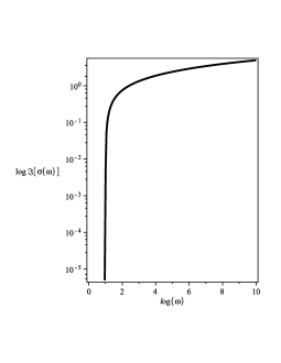
Figure 1: Variation of the $\log({{\mathfrak{Im}}}[{\sigma(\hat{\omega})}])$ for zero temperature limit in d=2.

so for the electromagnetic field we’ve

$$A(z)\approx C\frac{\sqrt[4]{b}}{\sqrt{i\pi r_{+}\hat{\omega}}}\Big{[}\frac{i\sqrt{z}}{\hat{\omega}r_{+}}-2+\frac{7}{3}i\frac{\hat{\omega}r_{+}}{\sqrt{z}}-\frac{\hat{\omega}^{2}r_{+}^{2}}{z}\Big{]}$$ (61)

Finally, we obtain the conductivity using (56) by the following simple formula

$$\sigma(\hat{\omega})=\frac{1}{2i\hat{\omega}}+\frac{i\hat{\omega}}{2}$$ (62)

Where as we guess ${{\mathfrak{Re}}}[{\sigma(\hat{\omega})}]=0$. The figure shows ${{\mathfrak{Im}}}[{\sigma(\hat{\omega})}]$ as a function of the $\hat{\omega}$ for zero temperature case and in $d=2$. The (62) gives the expression for DC conductivity in the zero temperature limit in $AdS_{2}/CFT_{1}$ model. Indeed, it’s comparable with the numerical results of the previous papers about one dimensional holographic superconductors Ren .

VIII Conclusion

In this paper, we investigated the analytical properties of a holographic superconductor with power Maxwell’s field. We studied the problem in the probe limit. We observed that it is possible to find the critical temperature $T_{c}$ and the condensation $<O_{+}>$ and the conductivity $\sigma(\omega)$ via Sturm-Liouville variational approach. We concluded that in $d=4$, when the power $\delta$ decreases, the value of the $<O_{+}>$ increases. Thus we can say that the effect of the power $\delta$ in $d=4$ model is in the direction of the increase of $<O_{+}>$. In $d=5$ when the power $\delta$ increases, the value of the $<O_{+}>$ increases. Thus, we can say that the effect of the power $\delta$ in $d=5$ model is in the direction of the increase of $<O_{+}>$. Further, we analytically deduced the low temperature and the zero-temperature DC conductivity $\sigma$ as a function of the $\hat{\omega}=\frac{\omega}{<O_{+}>^{\frac{1}{\Delta}}}$. Our work helps to giving a better understanding of some unfamiliar effects of the holographic superconductors both in different space dimensions and too on the effect of the non linearity in Maxwell’s strength field.

IX References

References

- (1) J. M. Maldacena, Adv. Theor. Math. Phys. 2, 231 (1998).
- (2) S. S. Gubser, I. R. Klebanov , A. M. Polyakov, Phys. Lett. B 428, 105 (1998).
- (3) E. Witten, Adv. Theor. Math. Phys. 2, 253 (1998).
- (4) C.P. Herzog, J. Phys. A 42,343001 (2009) .
- (5) S.A. Hartnoll, Class. Quant. Grav. 26,224002(2009).
- (6) G. Policastro, D. T. Son, and A. O. Starinets, Phys. Rev. Lett. 87, 081601 (2001).
- (7) P. Kovtun, D. T. Son, A. O. Starinets, JHEP 10,064(2003).
- (8) S.A. Hartnoll, C.P. Herzog , G.T. Horowitz, Phys. Rev. Lett. 101,031601 (2008).
- (9) P. Breitenlohner, D.Z. Freedman, Ann. Phys. 144, 249(1982).
- (10) S. S. Gubser, Phys.Rev.D78:065034 (2008),arXiv:0801.2977.
- (11) X. H. Ge, B. Wang, S. F. Wu , G. H. Yang, JHEP 1008, 108 (2010).
- (12) H. F. Li, R. G. Cai,H. Q. Zhang, JHEP 1104, 028 (2011).
- (13) R. G. Cai, H. F. Li , H. Q. Zhang, Phys. Rev. D 83, 126007 (2011).
- (14) C. M. Chen , M. F. Wu, arXiv:1103.5130.
- (15) X. H. Ge, arXiv:1105.4333.
- (16) M. R. Setare, D. Momeni, R. Myrzakulov, M. Raza, Phys. Scr. 86 , 045005 (2012),arXiv:1210.1062.
- (17) D. Momeni, M. R. Setare, N. Majd, JHEP05,118 (2011),arXiv:1003.0376
- (18) G. Siopsis , J. Therrien,arXiv:1011.2938.
- (19) H. B. Zeng, X. Gao, Y. Jiang , H. S. Zong, JHEP 1105, 002 (2011).
- (20) S. Gangopadhyay, D. Roychowdhury ,JHEP 08 (2012) 104.
- (21) M. R. Setare , D. Momeni, EPL, 96, 60006(2011),arXiv:1106.1025.
- (22) D. Momeni, E. Nakano, M. R. Setare , W.-Y. Wen, arXiv:1108.4340.
- (23) E. Nakano , Wen-Yu Wen, Phys. Rev. D 78, 046004 (2008).
- (24) T. Albash , C. V. Johnson, JHEP 0809, 121 (2008).
- (25) O. Domenech, M. Montull, A. Pomarol, A. Salvio, P. J. Silva,JHEP 1008:033,(2010),arXiv:1005.1776.
- (26) M. Montull, O. Pujolas, A. Salvio, P. J. Silva, arXiv:1105.5392.
- (27) M. Montull, O. Pujolas, A. Salvio, P. J. Silva, arXiv:1202.0006.
- (28) A. Salvio, arXiv:1207.3800.
- (29) N. Bobev, A. Kundu, K. Pilch, N. P. Warner, arXiv:1110.3454.
- (30) N. Bobev, N. Halmagyi, K. Pilch, N. P. Warner, arXiv:1006.2546.
- (31) N. Bobev, A. Kundu, K. Pilch, N. P. Warner, arXiv:1110.3454.
- (32) T. Fischbacher, K. Pilch, N. P. Warner, arXiv:1010.4910.
- (33) N. Bobev, A. Kundu, K. Pilch, N. P. Warner, arXiv:1110.3454.
- (34) D. Roychowdhury, Phys. Lett. B 718 ,1089(2013).
- (35) D. Roychowdhury,Phys Rev D 86, 106009 (2012).
- (36) R. Banerjee, S. Gangopadhyay, D. Roychowdhury, A. Lala, arXiv:1208.5902 .
- (37) S. Gangopadhyay, D. Roychowdhury, JHEP05(2012)156.
- (38) S. Gangopadhyay, D. Roychowdhury,JHEP05(2012)002.
- (39) J.-P. Wu, Y. Cao, X.-M. Kuang, W.-J. Li, Phys. Lett. B697, 153, (2011).
- (40) D. Momeni, M. R. Setare, Mod. Phys. Lett. A 26, 2889, (2011),arXiv:1106.0431.
- (41) D. Momeni, M. R. Setare, R. Myrzakulov, Int. J. Mod. Phys. A27, 1250128 (2012) ,arXiv:1209.3104.
- (42) D. Momeni, N. Majd, R. Myrzakulov,EPL, 97, 61001 (2012),arXiv:1204.1246.
- (43) S. Nojiri, S. D. Odintsov,Phys.Lett.B463,57, (1999)[hep-th/9904146]
- (44) S. Nojiri, S. D. Odintsov, Mod.Phys.Lett.A13:2695 (1998)[arXiv:gr-qc/9806034].
- (45) S. A. Hayward, Class. Quant. Grav. 15, 3147 (1998).
- (46) S. Nojiri, S. D. Odintsov, Phys.Rev.D59,044003(1999)[arXiv:hep-th/9806055].
- (47) J. Jing, Q. Pan, S. Chen, JHEP 1111, 045(2011) .
- (48) Q. Pan, J. Jing, B. Wang, arXiv: 1111.0714.
- (49) S. H. Mazharimousavi, M. Halilsoy, Phys. Rev. D 84, 064032 (2011).
- (50) M. Born , L. Infeld, Proc. R. Soc. A 144 , 425(1934).
- (51) Yu.N. Obukhov, Phys. Lett.A, 90, 13(1982).
- (52) Q. Pan, J. Jing, and B. Wang, Phys.Rev. D84 (2011).
- (53) S. Kanno, Class. Quant. Grav.28, 127001(2011).
- (54) G. T. Horowitz, M. M. Roberts, Phys. Rev. D 78 (2008) 126008.
- (55) M. Abramowitz, , I. Stegun, Handbook of Mathematical Functions. New York: Dover(1972).
- (56) Ronveaux, A. ed. Heun’s Differential Equations. Oxford University Press(1995).
- (57) J. Ren,JHEP 1011:055(2010),arXiv:1008.3904.