Hartree-Fock calculations for the photoionisation of helium and helium-like ions in neutron star magnetic fields

Abstract

We derive the photoionisation cross section in dipole approximation for many-electron atoms and ions for neutron star magnetic field strengths in the range of $10^{7}$ to $10^{9}$ T. Both bound and continuum states are treated in adiabatic approximation in a self-consistent way. Bound states are calculated by solving the Hartree-Fock-Roothaan equations using finite-element and $B$-spline techniques while the continuum orbital is calculated by direct integration of the Hartree-Fock equations in the mean-field potential of the remaining bound orbitals. We take into account mass and photon density in the neutron star’s atmosphere, finite nuclear mass as well as thermal occupation of the levels. The data may be of importance for the quantitative interpretation of observed x-ray spectra that originate from the thermal emission of isolated neutron stars. They can serve as input for modeling neutron star atmospheres as regards chemical composition, magnetic field strength, temperature, and redshift. Our main focus in this paper lies on helium and helium-like oxygen. These two-electron systems are simple enough to calculate all possible transitions when limiting the quantum numbers and should show all the basic structures and behaviour of other two-electron systems up to iron.

1 Introduction

Atoms in neutron star magnetic fields have been the subject of research for almost 40 years, starting with the analysis of the simplest chemical element, the hydrogen atom. A historical review of the work on the hydrogen atom in strong magnetic fields can be found in the book by Ruder et al. (Ruder et al., 1994). In particular, in the early 1980’s bound-bound (Ruder et al., 1994) as well as bound-free (Schmitt et al., 1981) transitions of hydrogen in strong magnetic fields were calculated.

Studies of heavier elements have received renewed impetus from the discovery of broad absorption features in the thermal X-ray emission spectra of the isolated neutron star 1E 1207.4-5209 (Sanwal et al., 2002; Mereghetti et al., 2002; Bignami et al., 2004) and three other isolated neutron stars (Haberl et al., 2003, 2004; van Kerkwijk et al., 2004) by the Chandra X-Ray Observatory of NASA and the XMM-Newton Observatory of ESA. These features could be of atomic origin (Mori & Hailey, 2002; Mori et al., 2005; Mori & Hailey, 2006). As can be seen from the review article on neutron star thermal emission by Zavlin (Zavlin, 2009), magnetized models of neutron star atmospheres have largely been confined to hydrogen atmospheres, partially or fully ionised. There were just a few attempts in the literature to model magnetized heavy element (carbon, oxygen, neon, iron) atmospheres. One attempt was undertaken by Mori and Ho (Ho & Mori, 2007). They showed that the features observed in 1E 1207 could be due to transitions of oxygen in different ionisation stages. Pavlov and Bezchastnov (Pavlov & Bezchastnov, 2005) suggested that the features can be produced by bound-bound transitions of singly ionised helium in strong magnetic fields. As noted by Zavlin and Pavlov (Zavlin & Pavlov, 2002), Rajagopal et al (Rajagopal et al., 1997) tried to model an iron atmosphere "‘with the use of rather crude approximations for the very complicated properties of iron ions in strong magnetic fields."’ A further interpretation in terms of peaks in the energy dependence of the free-free opacity has been put forward by Suleimanov et al. (Suleimanov et al., 2010), but again their modelling is restricted to hydrogen atmospheres.

In view of the unknown chemical compositions of the atmospheres of neutron stars, any possible fusion product, i.e., all elements from hydrogen to iron in various ionisation stages, could produce features in the thermal emission spectra of neutron stars. In order to be in a position to calculate synthetic spectra for models of neutron star atmospheres and to compare with observed spectra, in principle a complete knowledge of both the bound-bound transitions and the bound-free transitions of all these elements in strong magnetic fields, and in all ionisation stages, would be required. While bound-bound transitions in many-electron systems in neutron star magnetic field strengths have already been investigated in the literature (Engel & Wunner, 2008), calculations of photoionisation cross sections are few. Medin, Lai, and Potekhin (Medin et al., 2008) calculated a small number of bound-free transitions for helium in strong magnetic fields, as did Mori and Hailey (Mori & Hailey, 2006) for oxygen and neon ions.

We wish to extend these calculations by performing a systematic and complete study of the total photoionisation cross sections of two-electron atoms for the physically realistic situation that the initial bound states are thermally occupied, and the atoms are exposed to black body radiation of the same temperature. As in (Medin et al., 2008) we work with the adiabatic approximation (Schiff & Snyder, 1939; Canuto & Kelly, 1972) which implies that all electrons are in the lowest Landau level ($n=0$), with different magnetic quantum numbers ($m=0,-1,-2,-3,\cdots$), and the parts of the wave functions along the magnetic field are calculated self-consistently. (Adiabatic means, intuitively speaking, that the motion of the electrons in the plane perpendicular to the field is fast compared to the motion along the field, in which the electrons only feel the Coulomb potential of the nucleus, averaged over Landau orbitals.) In the low filed regime it is absolutely necessary to perform non-adiabatic calculations for bound states, as has been done, e.g. by (Becken et al., 1999; Schimeczek et al., 2012) but in the range of magnetic fields considered in this paper, the adiabatic approximation is applicable for bound states. Also the unbound state is accurately described in adiabatic approximation despite the strength of the magnetic field as long as its energy does not exceed the landau excitation threshold. The only effect appearing in a non-adiabatic treatment, is resonance of higher Landau-levels for bound-free transitions (Potekhin et al., 1997). But these resonances are much too high to be thermally excited ($\approx 10$ keV).

The specific difficulty in calculating photoionisation cross sections of many-electron atoms in strong magnetic fields lies in the lacking shell structure of these atoms. For every magnetic quantum number $m$ possible in the lowest Landau level there exists an energetically strongly lowered ground state (tightly bound state), while the energies of the excited states for every $m$ form a Rydberg series (hydrogen-like states). Thus all excited states are practically $m$-degenerate, and, assuming thermal occupation of the initial states, occupied with equal probability. The summation of the individual cross sections for the ionisation of the atoms from the $m$-degenerate states by photons of given energy would therefore diverge. We will introduce a physically reasonable cut-off criterion to avoid the divergence.

It is the purpose of this paper to demonstrate that we have developed a powerful tool for calculating practically complete photoionisation cross sections without the need to compromise accuracy for speed. These cross sections can serve as input for the computation of opacities and for more detailed astrophysical modelings.

The organisation of the paper is as follows: In Sec. 2, we briefly recapitulate the properties of atoms in intense magnetic fields and review the Hartree-Fock-Finite-Elements Roothaan (HFFER) method used to determine the bound initial states. The orbitals of the resulting ion and of the continuum electron after the photoionisation are calculated separately and then combined to a Slater determinant characterising the final state. The cross sections are derived in Sec. 3. Atomic data for helium and helium-like oxygen are presented in Sec. 4. The influences of photon and mass density, finite nuclear mass and thermal occupation are discussed in Sec. 5.

2 Atoms in very strong magnetic fields

For the readers’ convenience we briefly review the basics of atoms in strong magnetic fields (Ruder et al., 1994). A magnetic field $B$ is called strong if it exceeds the characteristic field strength $B_{0}=4.70108\times 10^{5}$ T, i.e., when the magnetic field parameter $\beta=B/B_{0}$ is large. In our calculations we will concentrate on a magnetic field strength of $B=10^{8}$ T which corresponds to $\beta\approx 212$. At $B_{0}$ the Larmor radius $a_{\rm L}$ becomes equal to the Bohr radius $a_{0}$. We note that $a_{\rm L}=a_{0}/\sqrt{\beta}$.

In strong fields the cylindrical symmetry of the magnetic field dominates, and it is therefore appropriate to work in cylindrical coordinates (we assume the field to point in the $z$ direction). Then we can write the Hamiltonian for an $N$-electron atom or ion with nuclear charge $Z$ (in atomic Rydberg units, i.e., $\hbar=4\pi\varepsilon_{0}=2m_{e}=e^{2}/2\equiv 1$) in the form $H=\sum_{i}^{N}\hat{H_{i}}\,$, with

$$\hat{H_{i}}=-\left(\frac{\partial^{2}}{\partial\rho_{i}^{2}}+\frac{1}{\rho_{i}}\frac{\partial}{\partial\rho_{i}}+\frac{1}{\rho_{i}^{2}}\frac{\partial^{2}}{\partial\phi_{i}^{2}}+\frac{\partial^{2}}{\partial z_{i}^{2}}\right)\mathds{1}\\ -2\,\mathrm{i}\,\beta\frac{\partial}{\partial\phi_{i}}\mathds{1}+\beta^{2}\rho_{i}^{2}\mathds{1}+2\beta\hat{\sigma}_{z,i}-\frac{2Z}{|\mathbf{r}_{i}|}\mathds{1}\\ +\frac{1}{2}\sum_{j\neq i}^{N}\frac{2}{|\mathbf{r}_{i}-\mathbf{r}_{j}|}\mathds{1}\,$$ (1)

being the Hamiltonian for the $i$-th electron. In (1) $\hat{\sigma}_{z}$ is the $z$ Pauli-matrix, and the term describes the interaction of the spin magnetic moment with the external field. At the magnetic field strength we consider, $B=10^{8}$ T, the splin flip energy, which is also the Landau excitation energy, amounts to $11.6$ keV, which is much larger than any single-orbital energy that we will encounter. Therefore it is justified to assume all electron spins to be aligned antiparallel to the magnetic field, and all single-electron states to occupy the lowest Landau level $n=0$. The spin part of the state will be omitted in what follows.

The single-particle orbital of electron $i$ is given by

$$\Psi_{i}(\rho,\phi,z)=\Phi_{m_{i}}(\rho,\phi)g_{m_{i}\nu_{i}}(z)\,,$$ (2)

where $\Phi_{m_{i}}(\rho,\phi)$ is the lowest Landau orbital, with magnetic quantum number $m_{i}$, and $g_{m_{i}\nu_{i}}(z)$ denotes the longitudinal part of the wave function. The quantum number $\nu_{i}$ counts the number of nodes of the wave function along the $z$ direction. In the following, states with quantum numbers $m$ and $\nu$ will be denoted by $(m,\nu)$. Recall that in the lowest Landau level $m$ only assumes non-positive values, $m=0,-1,-2,-3,\cdots$.

From the single-electron orbitals (2) of the bound electrons a Slater determinant is constructed, and the wave functions $g_{m_{i}\nu_{i}}(z)$ are determined self-consistently by solving the resulting Hartree-Fock equations. In our calculations, the $z$ axis is divided into finite elements, and the longitudinal wave functions are expanded in terms of $B$-splines. The $B$-spline expansion coefficients are determined by minimising the total energy functional (for computational details of this HFFER method cf. (Engel et al., 2009; Schimeczek et al., 2012)).

The final state of the bound-free transition consists of the ionised core and the electron which is photoionised into the continuum. Near the atomic core the unbound electron is influenced by the bound electrons, while the bound electrons can be assumed to be unaffected by the unbound electron (Medin et al., 2008). Therefore the initial state of the atom and the bound part of the final state, i.e., the ionised core, can be calculated separately in advance by the above mentioned method.

The wave function of the continuum electron is calculated by solving the Hartree-Fock equations that result from its interaction with the electrons of the remaining core:

$$\biggl{[}-\frac{\partial^{2}}{\partial z^{2}}+V_{m}(z)-E^{\prime}\\ +\sum_{j=1}^{N-1}\int\!\!\mathrm{d}z^{\prime}|g_{m_{j}\nu_{j}}(z^{\prime})|^{2}U_{m_{j}m}(z,z^{\prime})\biggr{]}g_{mE^{\prime}}(z)\\ =\!\!\sum_{j=1}^{N-1}\int\!\!\mathrm{d}z^{\prime}g_{mE^{\prime}}(z^{\prime})g_{m_{j}\nu_{j}}(z^{\prime})A_{m_{j}m}(z,z^{\prime})\times\\ \times g_{m_{j}\nu_{j}}(z)\,.$$ (3)

Here $V_{m}(z)$ represents the effective electron-core potential, $U_{mm^{\prime}}(z)$ and $A_{mm^{\prime}}(z)$ denote the effective electron-electron potential and the exchange potential, respectively. Their explicit forms are given in Appendix A. The energy $E^{\prime}$ replaces the number of nodes $\nu$ and is characteristic of the unbound electron.

The Hartree-Fock equations (3) are solved, for every given value of the continuum energy $E^{\prime}$, using a standard Runge-Kutta integrator. Since the $z$ parity is a good quantum number, one can calculate a symmetric and an antisymmetric wave function by imposing corresponding initial conditions at $z=0$. For $z\rightarrow\pm\infty$ these wave functions assume a sinusoidal shape, close to the nucleus both the amplitude and the period decrease due to the interaction with the ionic core and the bound electrons. Because of the delocalised nature of the continuum wave functions they can be normalised only over a finite periodicity length $d_{z}$. The latter, however, does not enter into the final results

3 Cross section for the photoionisation

In this section we give the formula for the photoionisation for the case that both the initial state $\psi_{\text{i}}$ and final state $\psi_{\text{f}}$ are Slater determinants. The former is composed of $N$ bound states, the latter consists of $N-1$ bound and one unbound wave function. The Hamiltonian $\hat{H}_{\text{int}}$ for the interaction of the electrons with the radiation field $\mathbf{A}_{\text{r}}~{}(\propto\boldsymbol{\varepsilon}\,\mathrm{e}^{\,\mathrm{i}\,\mathbf{k}\mathbf{r}})$ of the incoming photon is obtained by the usual minimal substitution of the momenta, $\mathbf{p}_{i}\to\boldsymbol{\pi}_{i}=\mathbf{p}_{i}-\sqrt{2}\mathbf{A}_{\text{r}}$ (recall that in atomic Rydberg units $e=\sqrt{2}$), and by taking into account the interaction of the spin magnetic moments of the electrons with the magnetic field $\mathbf{B}_{\rm r}=\nabla\times\mathbf{A}_{\text{r}}$ of the radiation field:

$$\hat{H}_{\text{int}}=\sum_{i=1}^{N}(2\boldsymbol{\beta}_{\text{r}}\mathbf{\hat{\boldsymbol{\sigma}}}_{i}-2\sqrt{2}\mathbf{A}_{\text{r}}{\boldsymbol{\pi}_{i}})\mathds{1}.$$ (4)

In (4), $\boldsymbol{\beta}_{\text{r}}=\mathbf{B}_{\rm r}/B_{0}$, and since we are interested in one-photon transitions the term quadratic in the vector potential has been omitted. The (one-dimensional) density of final states of the emitted (spin-down) electron is given by

$$\rho_{\text{f}}=\frac{d_{z}}{2\pi}\sqrt{\frac{1}{4E^{\prime}}}\,$$

where $d_{z}$ denotes the periodicity length in $z$-direction.

Starting from Fermi’s golden rule for the transition rate $w(\Psi_{\rm f},\Psi_{\rm i})=2\pi\left|\langle\Psi_{\rm f}|\hat{H}_{\text{int}}|\Psi_{\rm i}\rangle\right|^{2}\rho_{\text{f}}$, we can calculate the cross section by the usual relation $w=j\sigma$, with $j=c/V$ the photon flux of the incident radiation. Noting that in atomic Rydberg units $c=2/\alpha$, where $\alpha$ is the fine-structure constant, we have the relation $\sigma=\frac{V\alpha}{2}w$.

We calculate the photoionisation cross sections in dipole approximation. Therefore there are three types of transitions, which differ in the change of the total angular momentum in $z$ direction (quantum number $M=\sum m_{i}$) caused by the absorption of the photon. Linearly, right, and left circularly polarised light induces transitions, with $\Delta M=0$ ($\sigma_{0}$), $\Delta M=+1$ ($\sigma_{+}$) and $\Delta M=-1$ ($\sigma_{-}$), respectively.

It was shown in (Potekhin et al., 1997) that in the ’length form’ the cross sections in adiabatic and non-adiabatic form coincide. Therefore we also switch from the ’velocity form’ to the ’length form’ using the well known commutator relation

$$[\hat{H}_{i},\mathbf{r}_{i}]=-2\,\mathrm{i}\,\boldsymbol{\pi}_{i}\,,$$

where $\hat{H}_{i}$ designates the non-interaction-Hamiltonian of the $i$-th electron, cf. (1).

Lengthy but straightforward calculations finally yield explicit expressions for the photoionisation cross sections of the three types of dipole transitions, which can be found in Appendix B.

4 Cross sections of two-electron systems

For reasons of simplicity we choose helium and helium-like oxygen to be the systems of interest to demonstrate our method of calculation. They are still simple enough to compute a huge amount of single cross sections in reasonable time, and are complex enough to draw conclusions for other elements.

4.1 Single Cross Section

As an example, we discuss six single cross sections of helium and compare them to previously calculated cross sections (Medin et al., 2008). We will show that our algorithm can reproduce and improve upon these results. All presented cross sections are transitions where the ground state (configuration $(0,0)(1,0)$) is the initial state.

Figure 1: (Color online) Single cross sections for the first six transitions from the ground state $(0,0)(1,0)$ with different polarisations. The magnetic filed is $B=10^{8}$ T. In comparison to (Medin et al., 2008) these cross sections show more detail for higher energies.

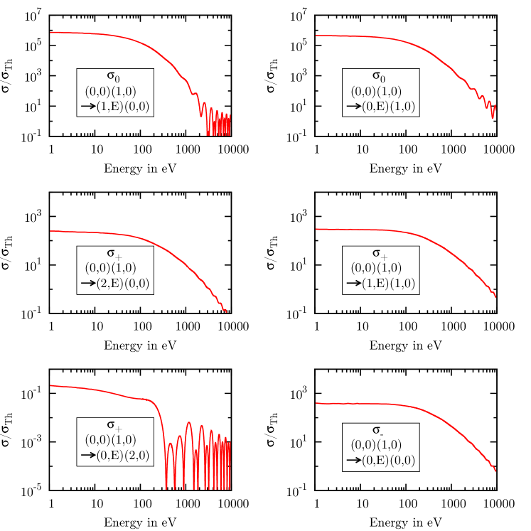
The six cross sections are shown in Figure 1, and are very similar to those calculated by Medin (see Figure .. in (Medin et al., 2008). However, there are differences in the low and high energy regime. For low energies, the values of the cross section are smaller as compared to those calculated by Medin et al.. Furthermore, from a certain energy on, the product of the bound and unbound wave functions becomes increasingly oscillating. This leads to a decline of the cross section and the occurrence of zero crossings.

We also have to analyse, what terms in the cross sections are important. For now the transition between the initial and the final state is given by $\left|g^{\mathrm{i}}_{m_{1}\nu_{1}}\right\rangle\left|g^{\mathrm{i}}_{m_{2}\nu_{2}}\right\rangle$ and $\left|g^{\mathrm{f}}_{m_{3}E^{\prime}}\right\rangle\left|g^{\mathrm{f}}_{m_{4}\nu_{4}}\right\rangle$. For two-electron atoms the double sum in (B1) reduces to four possible terms, two with the continuum wave function in the dipole matrix element, and two with the continuum wave function in the minor:

$$\begin{split}\left\langle g^{\mathrm{f}}_{m_{3}E^{\prime}}\left|\,z_{1}\,\right|g^{\mathrm{i}}_{m_{1}\nu_{1}}\right\rangle\delta_{m_{3},m_{1}}a^{\mathrm{fi}}_{31}\\ +\left\langle g^{\mathrm{f}}_{m_{3}E^{\prime}}\left|\,z_{2}\,\right|g^{\mathrm{i}}_{m_{2}\nu_{2}}\right\rangle\delta_{m_{3},m_{2}}a^{\mathrm{fi}}_{32}\\ +\left\langle g^{\mathrm{f}}_{m_{4}\nu_{4}}\left|\,z_{1}\,\right|g^{\mathrm{i}}_{m_{1}\nu_{1}}\right\rangle\delta_{m_{4},m_{1}}a^{\mathrm{fi}}_{41}\\ +\left\langle g^{\mathrm{f}}_{m_{4}\nu_{4}}\left|\,z_{2}\,\right|g^{\mathrm{i}}_{m_{2}\nu_{2}}\right\rangle\delta_{m_{4},m_{2}}a^{\mathrm{fi}}_{42}\end{split}$$ (5)

The behaviour of single cross sections is mainly determined by the unbound wave function. Since $z$-parity is a good quantum number the wave function is either symmetric or antisymmetric. In the transitions considered both single-particle orbitals of the initial state are symmetric. Therefore, if the continuum wave function appears in the minor, as is the case for the last two terms in (5), the latter has a value different from zero only for the symmetric continuum wave function. On the other hand, does the continuum wave function appear in the dipole matrix element, as is the case for the first two terms in (5), only the antisymmetric continuum wave function yields a nonvanishing contribution because of the antisymmetry of the operator $z$. So generally only two of the four terms are important for one cross section.

Figure 2: (Color online) Symmetric and antisymmetric continuum wave functions of helium for the state $(m_{3}=1,E^{\prime}=0.1~{}\rm{eV})\ (m_{4}=0,\nu_{4}=0)$ at $B=10^{8}$ T ($\beta\approx 212$).

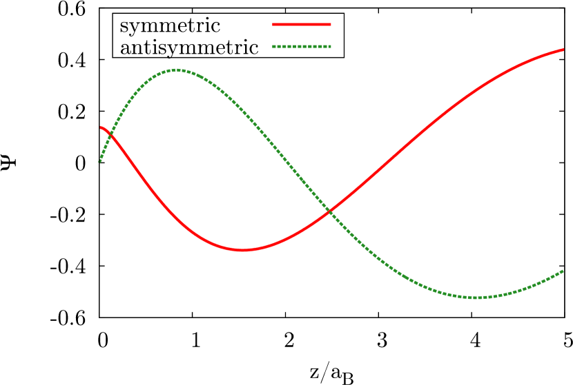
If we take a look at a typical wave function like the one presented in Figure 2, we can see that the form of the symmetric and the antisymmetric continuum wave function near zero is very different. In this region, the value of the cross section is determined by the form of the bound wave function and attains a high value when both the bound and continuum wave function coincide in their shapes.

4.2 Total Cross Section

We now wish to calculate the total cross section for the ionisation by a photon of a given energy, which is the sum over all single cross sections $\sigma=\sum_{i}\sigma_{i}$. Since in the lowest Landau level the magnetic quantum numbers in principle are not bounded below, this sum would diverge. To find a physically reasonable cut-off we make use of the fact that the spatial extension $\rho_{0}$ of a Landau state $\Phi_{m}(\rho,\phi)$ is characterized by (Canuto & Ventura, 1977)

$$\rho_{0}^{2}=a_{L}^{2}\left(|m|+\frac{1}{2}\right)$$ (6)

with $a_{L}=a_{0}/\sqrt{\beta}$ the Larmor radius. This means that as $|m|$ increases the atoms become broader and broader in the direction perpendicular to the field until, at a given mass density, for some $|m|$ they begin to ”touch” each other. This determines the maximum magnetic quantum number that has to be considered when summing for the total cross section. In the results presented below we chose a maximum value of $\left\lvert\,m\,\right\rvert=200$. In an analogous fashion we restrict ourselves to longitudinal wave functions with a maximum number of nodes $\nu=2$, since for larger number of nodes the orbitals would overlap at a given mass density. In Section V we will give values for the mass densities that are covered by these restrictions.

We note that with this the number of initial states amounts 180,300. Starting from these states, every possible transition has to be found. For every polarisation, these states lead in total to roughly 1 million transitions. In Fig. 3 we compare the total cross section of helium, summed over all possible ionisations, and helium-like oxygen.

Figure 3: (Color online) Left: Total cross section for the photoionisation of helium at $B=10^{8}$ T obtained by summing over all initial states with $|m|\leq 200$ and $\nu\leq 2$ as a function of the photon energy for the three different polarisations. Right: The corresponding cross section for helium-like oxygen.

In both cases, the cross sections with circularly polarised light are several orders of magnitude smaller than the cross section with linearly polarised light. Also the general behavior of the curves for both elements is similar. The main difference is the position of the maximum cross section. As can be expected, the maximum for oxygen is at higher energies, due to the higher binding energy. The second difference is the absolute value, which is smaller for oxygen.

5 Cross section for realistic physical conditions of a neutron star

In this section we calculate effective photoionisation cross sections by taking into account the physical conditions that prevail in the neutron star atmosphere. First we assume a thermal occupation of the initial states and calculate total cross sections as a function of photon energy. Then we determine cross sections averaged over the photon energies of a Planckian spectrum. Finally we explore the effects of the plasma density and estimate the values for the mass density for which the cut-off criteria are valid.

5.1 Thermal occupation probability

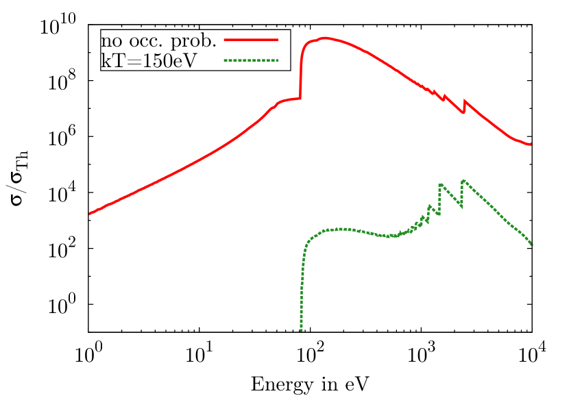
Neutron star atmospheres are hot, with temperatures up to $10^{6}$ K (Zavlin, 2009). We account for this fact by a thermal occupation of the initial states, and in summing the single photoionisation cross sections weight their contributions to the total cross section according to their occupation probability $p(E)=e^{-\Delta E/kT}$. From (Mori & Hailey, 2006) and (Bignami et al., 2002) we adopt a representative value of $kT=150$ eV and, to demonstrate the influence of an increase of temperature, of $kT=300$ eV.

Figure 4: (Color online) Total cross section for the photoionisation of helium at $B=10^{8}$ T as a function of the photon energy for linear polarisation obtained by summing over all initial states with $|m|\leq 200$ and $\nu\leq 2$ and assuming thermal occupation of the initial states. The cross section without thermal occupation from Fig. 3 is shown for comparison.

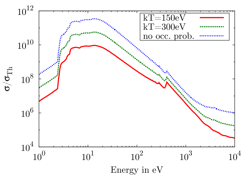
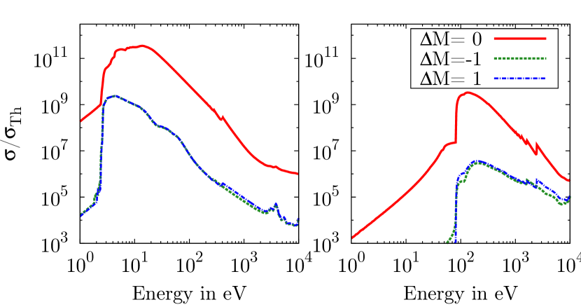
The resulting cross sections are shown in Fig. 4. At higher temperatures the occupation probabilities of the excited bound states are larger, which yields an increase of the total cross section. Also, without thermal occupation weighting the cross section was much larger. We have the effect that single cross sections of excited initial states which manifested themselves at lower energies can be rather large, but are suppressed if thermal occupation probability is taken into account.

This effect becomes even more pronounced when we proceed to heavier elements such as oxygen (see Fig. 5). Below 100 eV practically no transitions contribute, and the peak around 100 eV becomes suppressed. The reason is that the energy difference between excited states and the ground state of oxygen is much larger than for helium, therefore the occupation probability is very small. In fact, we can show that there are only 600 transitions left which contribute significantly to the cross section. All other transitions are negligible.

Figure 5: (Color online) As Fig. 4 but for helium-like oxygen.

In the following, we concentrate on the total cross section for thermal occupation of the initial states with $kT=150$ eV. Circularly polarised light is not considered in particular since it shows the same qualitative behavior as linearly polarised light.

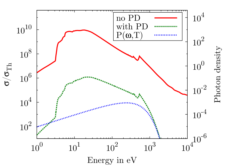
5.2 Photon density

We now take into account the temperature dependent spectral distribution of photons in the neutron star atmosphere, which we assume to be blackbody, and calculate total cross sections averaged over the photon energy distribution. This is only a simple model, to illustrate the influence of the energy dependence of the incident photon flux. It is these cross sections which are needed for the astrophysical modeling of the spectra of thermally emitting magnetised neutron stars. The starting point is Planck’s law divided by the photon frequency and, due to the assumption of a photon flux with one photon per volume element, normalized by the factor

$$\int_{0}^{\infty}\tilde{P}(\omega,T)\mathrm{d}\omega=\frac{4\pi T^{3}}{\alpha^{3}}2\zeta(3)\ ,$$ (7)

where $\zeta(x)$ is the Riemann zeta function. This yields the photon density

$$P(\omega,T)\mathrm{d}\omega=\frac{\omega^{2}}{2\operatorname{\zeta}(3)T^{3}}\frac{1}{\,\mathrm{e}^{\omega/T}-1}\mathrm{d}\omega\,.$$ (8)

The resulting photon density is shown in Fig. 6, for the temperature of $kT=150$ eV.

The effect of the photon density is best shown in a comparison between the cross sections without photon density and the same cross section multiplied by the photon density $P(\omega)$ (Fig. 6). The cross section changes its qualitative behavior towards the shape of the photon density. The peaks at energies around 20 eV are suppressed and the decay at energies greater than 400 eV is more rapid due to the low photon density.

Figure 6: (Color online) Total cross section for the photoionisation of helium at $B=10^{8}$ T obtained by summing over all initial states with $|m|\leq 200$ and $\nu\leq 2$ for thermal occupation of the initial states with $kT=150$ eV, and averaged over a blackbody spectrum of the incident photon (linear polarisation) with the same temperature (lower dotted curve). The spectrally not averaged cross section from Fig. 4 (upper curve) is shown for comparison.

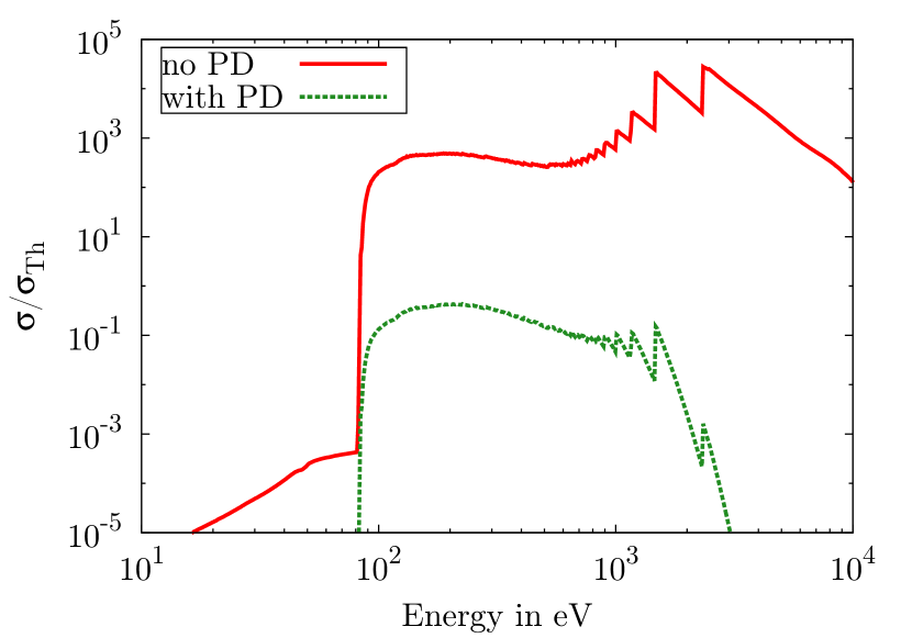
The same picture for helium-like oxygen shows intriguing behavior (Fig. 7). The last two peaks around 2 keV originally have about the same value. When the photon density is taken into account the last peak is two orders of magnitude smaller. Thus the photon density can change the the shape of the final total cross section significantly.

Figure 7: (Color online) As Fig. 6 but for helium-like oxygen at $B=10^{8}$ T.

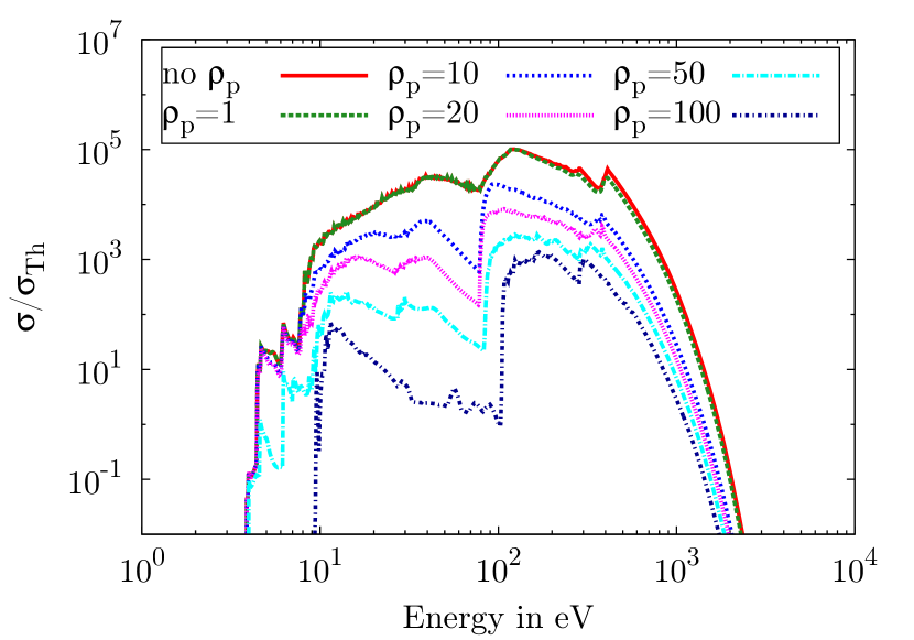
5.3 Density of the plasma

The atmosphere of a neutron star consists of ionised atoms. The volume an atom can fill is restricted by the particle density. Because of the enormous gravity at the surface neutron star atmospheres are strongly suppressed, and values for the mass density one finds in the literature range between $\varrho_{p}=1$ g/cm³ and $\varrho_{p}=100$ g/cm³ (see e.g. (Mori & Hailey, 2006; Zavlin, 2009)). Assuming that all atoms occupy the same state, the average volume available per atom $V_{s}$ can be written as $V_{s}={m_{\text{atom}}}/{\varrho_{p}}$ where $m_{\text{atom}}$ is the atomic mass. No overlap of adjacent atoms with volumes smaller than $V_{s}$ exists, and we have included only the contributions from these atomic states. We now wish to estimate for which mass densities in our calculations the restriction to $\left\lvert\,m\,\right\rvert\leq 200$ and $\nu\leq 2$ is justified, and whether or not for higher mass densities the maximum $\left\lvert\,m\,\right\rvert$ can even be decreased.

We make the simple approximation that the atoms are cylindrically shaped and aligned gaplessly. As already noted the spatial extension $\rho_{0}$ of a state perpendicular to the magnetic field is given by (6). We only consider the electron orbital with the largest extent, that is, with the maximum $\left\lvert\,m\,\right\rvert$. The corresponding volume of the atom is $V_{a}=2\pi\rho^{2}_{0}(|m|)\sqrt{\left\langle z^{2}\right\rangle_{\text{max}}}\ ,$ where $\sqrt{\left\langle z^{2}\right\rangle_{\text{max}}}$ denotes the maximum extension in $z$-direction. Generally, higher $\nu$ result in larger extensions. If the calculated volume $V_{a}$ is bigger than $V_{s}$, the state is omitted as an initial state. The same is true for final states.

In a more detailed treatment one would have to consider that the atoms are not purely cylindrical but cigar-shaped and therefore, more or less, aligned in an ellipsoidal packing. Moreover different states coexist, and the atoms are not aligned gaplessly but exhibit a separation. However, our simple approximation is good enough for the estimates that we are seeking For a more realistic approach, see e.g. (Hummer & Mihalas, 1988).

$\varrho$ in $\text{g}/\text{cm}^{3}$	$\nu$	highest $\left\lvert\,m\,\right\rvert$	$N_{t}$
	0	199
1	1	169	336 172
	2	125
	0	36
10	1	22	4 978
	2	15
	0	20
20	1	11	1 400
	2	7
	0	9
50	1	4	282
	2	2
	0	5
100	1	2	71
	2	1

Table 1: Highest $\left\lvert\,m\,\right\rvert$ depending on $\nu$ at different plasma densities and the total number of transitions $N_{t}$.

In Table 1 we list, for five different mass densities the maximum $\left\lvert\,m\,\right\rvert$ depending on $\nu$ for which the volume of this state is still small enough to contribute to the cross section. This maximum quantum number declines fast for higher densities. It is interesting to note that some volumes of states with $\nu=2$ at higher densities are still small enough. This is due to the very small $\rho_{0}$ if $m=0$, and for two electrons the interaction with the nucleus is very strong so that $\left\langle z^{2}\right\rangle$ increases only slowly. Therefore states with $m=0$ can still be small enough, even if $\nu$ becomes very large. This also implies, that we still do not have a complete total cross section, but due to the low $\left\lvert\,m\,\right\rvert$ and $\nu$ seen in Table 1, it is possible to calculate all states and transitions in reasonable time.

The Table also shows that the number of transitions that have to be considered when calculating the total cross section. This number decreases rapidly, until at 100 g/cm³ there is only 0.006% of the transitions necessary originally left.

Figure 8 shows the cross section, calculated for linearly polarised light, with mass densities between 1 and 100 g/cm³. It can be seen that at 1 g/cm³ the cross section changes only quantitatively, but not its qualitative behavior, while the number of transitions decreases by 740,000, which is 70% of the total transitions. The consequence is that many single cross section are negligible.

Figure 8: (Color online) Total photoionisation cross section of helium at $B=10^{8}$ T for linear polarisation obtained by summing only over as many initial states as are compatible with the mass density $\varrho_{p}$ (cf. Table 1). Values of $\varrho_{p}$ are given in $[\text{g}/\text{cm}^{3}]$. Thermal occupation of the initial states with $kT=150$ eV is assumed. The thermally averaged cross section from Fig. 4 in which the mass density is not taken into account (top most curve) is shown for comparison. It can be seen that as the density increases the cross sections significantly change in height and shape.

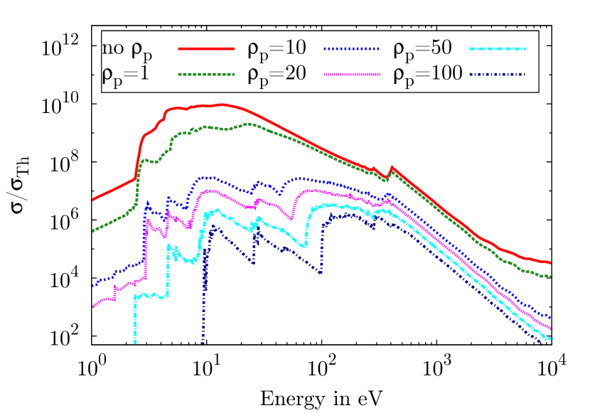
Starting at 10 g/cm³, the cross section is significantly changed. There is only a fraction of the originally calculated cross sections left, which is the reason for this huge change.

In particular, mostly highly excited states drop out. These transitions contribute to the lower energy range (1-50 eV) and this is why the cross section changes significantly in this range.

5.4 Finite Core Mass

In all our calculations we have worked in the infinite-nuclear-mass approximation. We therefore finally discuss the influence of the finite nucleus mass on the results. It has been shown (Wunner et al., 1980; Ruder et al., 1994) that the single-particle levels are raised by the cyclotron energy $\hbar\omega^{+}$ of the charged atomic nucleus. Intuitively this corresponds to its own gyration as a charged particle in the magnetic field.

This so called $m$-shift rises the energy levels of every state, so that many of these are shifted over the ionisation edge, and therefore need no longer be accounted for in the total cross section.

For the magnetic field strength considered here ($B=10^{8}$ T), $\hbar\omega^{+}=1.67$ eV for helium, and $0.39$ eV and $0.11$ eV for helium-like oxygen and iron, respectively. This does not influence transition energies with $\Delta M$ = 0, since all levels are raised by the same amount, and gives only a small correction for the, as compared to $\Delta M=0$, weaker transitions with $\Delta M=\pm 1$.

Figure 9: (Color online) The cross section for helium at $B=10^{8}$ T for linear polarisation and thermal weight at $kT=150$ eV with account for the finite nuclear mass. For comparison the total cross section with infinite nuclear mas is shown (upper curve).

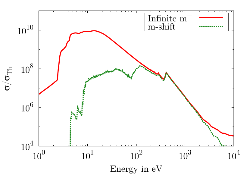
Figure 9 shows the total cross section calculated with finite nuclear mass. As was expected, the highly excited states are no longer accounted for, so mainly the low level transitions are dropping out. This behaviour is similar to the mass density effect.

The reduction of the number and composition of transitions is important when calculating opacities. If oversized and autoionising atoms are neglected, we know that no transitions are missing in the total cross section.

All physical conditions prevailing in the neutron star atmosphere are taken into account in Fig. 10, for a thermal occupation probability at $kT=150$ eV, the photon density $P(\omega)$ with $kT=150$ eV, different plasma densities and finite nuclear mass. The Figure shows that the peaks at energies between 10 and 50 eV are suppressed due to the low photon density, and the overall shift towards the shape of the photon density is obvious.

Figure 10: (Color online) As Fig. 8 but additionally with spectral averaging over a blackbody spectrum with $kT=150$ eV. Values of $\varrho_{p}$ are again given in $[\text{g}/\text{cm}^{3}]$.

We can again look at the number of transitions remaining for different plasma densities in Table 2. Here we are only interested in the total number, without the splitting into $\nu$-channels. A comparison quickly shows, that only few atoms that are not oversized drop out of the calculation. This does not mean that finite nuclear mass is negligible, but both effects have to be taken into account, for a complete cross section.

$\varrho$ in $\text{g}/\text{cm}^{3}$	$N_{t}$
1	44967
10	4506
20	1264
50	251
100	59

Table 2: The total number of transitions $N_{t}$ at different plasma densities with finite nuclear mass.

6 Summary

We have developed a program code which allows calculating bound-free transitions of few-electron atoms and ions in neutron star magnetic fields in a routine way. For the examples of helium and helium-like oxygen we have analysed, for realistic physical parameters, which transitions contribute significantly to the total photoionisation cross sections and which are negligible. In this way we have succeeded in drastically reducing the numbers of transitions that have to be considered. The strategies developed in reducing the number of contributing transitions can also be applied in the calculation of the photoionisation of atoms and ions with more than two electrons.

The present results clearly demonstrate the complexity of ab-initio calculations of realistic photoionisation cross sections in neutron star magnetic fields that can be used in astrophysical modeling. An alternative would be the development of phenomenological models for the cross sections. Here our results could serve as useful starting point for developing such models.

7 Acknowledgements

We thank the bwGRiD project (http://www.bw-grid.de), member of the German D-Grid initiative, funded by the Ministry for Education and Research (Bundesministerium für Bildung und Forschung) and the Ministry for Science, Research and Arts Baden-Württemberg (Ministerium für Wissenschaft, Forschung und Kunst Baden-Württemberg) for providing the computational resources, and Christoph Schimeczek and Sebastian Boblest for valuable discussions and input.

Appendix A Potentials

The explicit forms of the potetials in (3) read

$$V_{m}(z)= -2Z\int\text{d}\mathbf{r}_{\bot}\frac{|\Phi_{m}(\mathbf{r}_{\bot})|^{2}}{|\mathbf{r}|}\,,$$

$$U_{mm^{\prime}}(z,z^{\prime})= \ 2\iint\text{d}\mathbf{r}_{\bot}\text{d}\mathbf{r}_{\bot}^{{}^{\prime}}\frac{|\Phi_{m}(\mathbf{r}_{\bot})|^{2}|\Phi_{m^{\prime}}(\mathbf{r}_{\bot}^{{}^{\prime}})|^{2}}{|\mathbf{r}^{{}^{\prime}}-\mathbf{r}|}\,,$$

$$A_{mm^{\prime}}(z,z^{\prime})= \ 2\iint\text{d}\mathbf{r}_{\bot}\text{d}\mathbf{r}_{\bot}^{{}^{\prime}}\frac{\Phi_{m^{\prime}}^{*}(\mathbf{r}_{\bot})\Phi_{m}(\mathbf{r}_{\bot})\Phi_{m}^{*}(\mathbf{r}_{\bot}^{{}^{\prime}})\Phi_{m^{\prime}}(\mathbf{r}_{\bot}^{{}^{\prime}})}{|\mathbf{r}^{{}^{\prime}}-\mathbf{r}|}\,.$$

These three potentials can be computed numerically by evaluating the integrals. For a detailed description of the evaluation of the above integrals we refer to (Pröschel et al., 1982).

Appendix B Cross Section

The photoionization cross section of the three types of dipole transitions are

$$\begin{split}\sigma_{0}=&\frac{3}{8}\frac{d_{z}\sigma_{\text{Th}}\omega_{\mathrm{fi}}^{2}}{\alpha^{3}\omega_{\text{ph}}}\sqrt{\frac{1}{E^{\prime}}}\,\varepsilon_{z}^{2}\left|\,\sum_{k=1}^{N-1}\sum_{l=1}^{N}\left\langle g^{\mathrm{f}}_{m_{k}\nu_{k}}\left|\,z_{l}\,\right|g^{\mathrm{i}}_{m_{l}\nu_{l}}\right\rangle\delta_{m_{k},m_{l}}a^{\mathrm{fi}}_{kl}\right.\\ &\phantom{\frac{3}{8}\frac{d_{z}\sigma_{\text{Th}}\omega_{\mathrm{fi}}^{2}}{\alpha^{3}\omega_{\text{ph}}}\sqrt{\frac{1}{E^{\prime}}}\,\varepsilon_{z}^{2}\left|\,\sum_{k=1}^{N-1}\right.}+\left.\sum_{l=1}^{N}\left\langle g^{\mathrm{f}}_{m_{N}E^{\prime}}\left|\,z_{l}\,\right|g^{\mathrm{i}}_{m_{l}\nu_{l}}\right\rangle\delta_{m_{N},m_{l}}a^{\mathrm{fi}}_{Nl}\,\right|^{2}\\ \sigma_{-}=&\frac{3}{8}\frac{d_{z}\sigma_{\text{Th}}\omega_{\mathrm{fi}}^{2}}{\alpha^{3}\omega_{\text{ph}}}\sqrt{\frac{1}{E^{\prime}}}\left\lvert\,\varepsilon_{+}\,\right\rvert^{2}\left|\,\sum_{k=1}^{N-1}\sum_{l=1}^{N}\left\langle g^{\mathrm{f}}_{m_{k}{\nu_{k}}}\left|\,\sqrt{\frac{-m_{l}+1}{4\beta}}\,\right|g^{\mathrm{i}}_{m_{l}\nu_{l}}\right\rangle\delta_{m_{k}-1,m_{l}}a^{\mathrm{fi}}_{kl}\right.\\ &\phantom{\frac{3}{8}\frac{d_{z}\sigma_{\text{Th}}\omega_{\mathrm{fi}}^{2}}{\alpha^{3}\omega_{\text{ph}}}\sqrt{\frac{1}{E^{\prime}}}\,\varepsilon_{z}^{2}\left|\,\sum_{k=1}^{N-1}\right.}+\left.\sum_{l=1}^{N}\left\langle g^{\mathrm{f}}_{m_{N}E^{\prime}}\left|\,\sqrt{\frac{-m_{l}+1}{4\beta}}\,\right|g^{\mathrm{i}}_{m_{l}\nu_{l}}\right\rangle\delta_{m_{N}-1,m_{l}}a^{\mathrm{fi}}_{Nl}\,\right|^{2}\\ \sigma_{+}=&\frac{3}{8}\frac{d_{z}\sigma_{\text{Th}}\omega_{\mathrm{fi}}^{2}}{\alpha^{3}\omega_{\text{ph}}}\sqrt{\frac{1}{E^{\prime}}}\left\lvert\,\varepsilon_{-}\,\right\rvert^{2}\left|\,\sum_{k=1}^{N-1}\sum_{l=1}^{N}\left\langle g^{\mathrm{f}}_{m_{k}\nu_{k}}\left|\,\sqrt{\frac{-m_{l}}{4\beta}}\,\right|g^{\mathrm{i}}_{m_{l}\nu_{l}}\right\rangle\delta_{m_{k}+1,m_{l}}a^{\mathrm{fi}}_{kl}\right.\\ &\phantom{\frac{3}{8}\frac{d_{z}\sigma_{\text{Th}}\omega_{\mathrm{fi}}^{2}}{\alpha^{3}\omega_{\text{ph}}}\sqrt{\frac{1}{E^{\prime}}}\,\varepsilon_{z}^{2}\left|\,\sum_{k=1}^{N-1}\right.}+\left.\sum_{l=1}^{N}\left\langle g^{\mathrm{f}}_{m_{N}E^{\prime}}\left|\,\sqrt{\frac{-m_{l}}{4\beta}}\,\right|g^{\mathrm{i}}_{m_{l}\nu_{l}}\right\rangle\delta_{m_{N}+1,m_{l}}a^{\mathrm{fi}}_{Nl}\,\right|^{2}\,.\end{split}$$ (B1)

In (B1) $\omega_{\text{ph}}$ is the energy of the incident photon and $\sigma_{\text{Th}}=8\pi\alpha^{4}/3$ is the Thomson cross section.

The subdeterminant $a_{kl}^{\mathrm{fi}}$ is defined by $a_{kl}^{\mathrm{fi}}=(-1)^{k+l}\det(A_{kl})$, where $\det(A_{kl})$ is the minor (remove row $k$ and column $l$) of the matrix consisting of the elements $S_{kl}^{\mathrm{fi}}=\left\langle\psi_{\mathrm{f},k}\right|\left.\!\psi_{\mathrm{i},l}\right\rangle$, which represent the overlaps between the single-particle-orbitals $\psi_{\mathrm{i},l}$ and $\psi_{\mathrm{f},k}$.

A few remarks are in order regarding equation (B1). Since we do not take multi-photon transitions into account, we can replace the photon’s energy $\omega_{\text{ph}}$ by the energy difference between final and initial state $\omega_{\mathrm{fi}}$ ($\omega_{\text{ph}}=\omega_{\mathrm{fi}}$ for single-photon transitions). Although the periodicity length $d_{z}$ occurs in the formulae, the calculated cross sections are independent of $d_{z}$. This is due to the fact that the continuum wave function of the ionised electron is normalised with respect to $d_{z}$ and therefore contains a factor $1/\sqrt{d_{z}}$.

References

- Becken et al. (1999) Becken, W., Schmelcher, P., & Diakonos, F. 1999, OURNAL OF PHYSICS B-ATOMIC MOLECULAR AND OPTICAL PHYSICS, 32, 1557
- Bignami et al. (2002) Bignami, G., De Luca, A., Caraveo, P., et al. 2002, Memorie della Società Astronomica Italiana, 73
- Bignami et al. (2004) Bignami, G. F., De Luca, A., Caraveo, P. A., et al. 2004, Memories of the Italian Astronomical Society, 75, 448
- Canuto & Kelly (1972) Canuto, V., & Kelly, D. 1972, Astrophys. Sp. Sc., 17, 277
- Canuto & Ventura (1977) Canuto, V., & Ventura, J. 1977, Fundamentals of Cosmic Physics, 2, 203
- Engel et al. (2009) Engel, D., Klews, M., & Wunner, G. 2009, Comp. Phys. Comm., 180, 302
- Engel & Wunner (2008) Engel, D., & Wunner, G. 2008, Phys. Rev. A, 78, 032515
- Haberl et al. (2003) Haberl, F., Schwope, A. D., Hambaryan, V., Hasinger, G., & Motch, C. 2003, Astron. Astrophys., 403, L19
- Haberl et al. (2004) Haberl, F., Zavlin, V. E., Trümper, J., & Burwitz, V. 2004, Astron. Astrophys., 419, 1077
- Ho & Mori (2007) Ho, W. C. G., & Mori, K. 2007, Mon. Not. R. Astron. Soc., 377, 903
- Hummer & Mihalas (1988) Hummer, D., & Mihalas, D. 1988, Astrophys. J., 331, 794
- Medin et al. (2008) Medin, Z., Lai, D., & Potekhin, A. Y. 2008, Mon. Not. R. Astron. Soc., 383, 161–172
- Mereghetti et al. (2002) Mereghetti, S., Luca, A. D., Caraveo, P. A., et al. 2002, Astrophys. J., 581, 1280
- Mori et al. (2005) Mori, K., Chonko, J. C., & Hailey, C. J. 2005, Astrophys. J., 631, 1082
- Mori & Hailey (2002) Mori, K., & Hailey, C. J. 2002, Astrophys. J., 564, 914
- Mori & Hailey (2006) —. 2006, Astrophys. J., 648, 1139
- Pavlov & Bezchastnov (2005) Pavlov, G. G., & Bezchastnov, V. G. 2005, Astrophys. J., 635, L61
- Potekhin et al. (1997) Potekhin, A., Pavlov, G., & Ventura, J. 1997, ASTRONOMY & ASTROPHYSICS, 317, 618
- Pröschel et al. (1982) Pröschel, P., Rösner, W., Wunner, G., Ruder, H., & Herold, H. 1982, J. Phys. B: At. Mol Phys., 15, 1959
- Rajagopal et al. (1997) Rajagopal, M., Romani, R., & Miller, M. 1997, ASTROPHYSICAL JOURNAL, 479, 347
- Ruder et al. (1994) Ruder, H., Wunner, G., Herold, H., & Geyer, F. 1994, Atoms in Strong Magnetic Fields, Astronomy and Astrophysics Library (Springer-Verlag)
- Sanwal et al. (2002) Sanwal, D., Pavlov, G. G., Zavlin, V. E., & Teter, M. A. 2002, Astrophys. J., 574, L61
- Schiff & Snyder (1939) Schiff, L., & Snyder, H. 1939, Phys. Rev., 55, 0059
- Schimeczek et al. (2012) Schimeczek, C., Engel, D., & Wunner, G. 2012, Comp. Phys. Comm., 183, 1502
- Schmitt et al. (1981) Schmitt, W., Herold, W. H., Ruder, H., & Wunner, G. 1981, Astron. Astrophys., 94, 194
- Suleimanov et al. (2010) Suleimanov, V. F., Pavlov, G. G., & Werner, K. 2010, Astrophys. J., 714, 630
- van Kerkwijk et al. (2004) van Kerkwijk, M. H., Kaplan, D. L., Durant, M., Kulkarni, S. R., & Paerels, F. 2004, Astrophys. J., 608, 432
- Wunner et al. (1980) Wunner, G., Ruder, H., & Herold, H. 1980, Phys. Lett. A, 79, 159
- Zavlin & Pavlov (2002) Zavlin, V., & Pavlov, G. 2002, arXiv:astro-ph/0206025v1
- Zavlin (2009) Zavlin, V. E. 2009, in Astrophysics and Space Science Library, Vol. 357, Neutron Stars and Pulsars, ed. W. Becker (Heidelberg: Springer-Verlag), 181–211