Modified trigonometric integrators

Abstract

We study modified trigonometric integrators, which generalize the popular class of trigonometric integrators for highly oscillatory Hamiltonian systems by allowing the fast frequencies to be modified. Among all methods of this class, we show that the IMEX (implicit-explicit) method, which is equivalent to applying the midpoint rule to the fast, linear part of the system and the leapfrog (Störmer/Verlet) method to the slow, nonlinear part, is distinguished by the following properties: (i) it is symplectic; (ii) it is free of artificial resonances; (iii) it is the unique method that correctly captures slow energy exchange to leading order; (iv) it conserves the total energy and a modified oscillatory energy up to to second order; (v) it is uniformly second-order accurate in the slow components; and (vi) it has the correct magnitude of deviations of the fast oscillatory energy, which is an adiabatic invariant. These theoretical results are supported by numerical experiments on the Fermi–Pasta–Ulam problem and indicate that the IMEX method, for these six properties, dominates the class of modified trigonometric integrators.

1 Introduction

1.1 Overview

Over the past two decades, there has been considerable interest in so-called geometric numerical integrators, particularly symplectic integrators for Hamiltonian systems [10, 12]. In contrast to general-purpose numerical integrators, geometric integrators are designed especially to be applied to systems with some additional underlying structure (symmetries, invariants, etc.) that the algorithm must preserve exactly, at least up to round-off error.

While there have been many successes in this area, the integration of highly oscillatory Hamiltonian systems—which feature both stiff, linear forces and soft, nonlinear forces—has remained persistently difficult, due to the simultaneous presence of fast and slow time scales. Such systems are especially prevalent, for instance, in molecular dynamics, where one must contend with strong, short-range bonding forces, as well as weak, long-range electrostatic forces.

One of the main advances has been the development and analysis of trigonometric integrators, which are numerical methods designed especially to integrate certain highly oscillatory systems. However, these methods have certain drawbacks: in particular, there is a trade-off between numerical stability and consistency with respect to certain dynamical features, such as the emergent multiscale phenomenon of slow energy exchange and the near-preservation of adiabatic invariants.

In this paper, we show that modified trigonometric integrators—that is, trigonometric integrators with modified oscillatory frequencies—provide a way around this obstacle. Naively, one might expect that perturbing the frequency would increase the error, so it may seem counterintuitive to suggest that this can actually improve numerical performance. Yet, we show that this is indeed the case: allowing for the frequency to be modified provides an additional degree of freedom, which makes it possible to sidestep the aforementioned trade-off between stability and multiscale structure preservation. Specifically, we show that a particular, unique choice of modified frequency yields an integrator that is both stable and structure-preserving, and this is precisely the implicit-explicit (IMEX) method of Stern and Grinspun [15].

1.2 The numerical challenge of fast oscillations

Consider a prototypical highly oscillatory problem, given by the second-order equation

(1) $$\ddot{q}+\Omega^{2}q=g(q),$$

where $q(t)\in\mathbb{R}^{d}$ is a trajectory, $\Omega=\bigl{(}\begin{smallmatrix}0&0\\ 0&\omega I\end{smallmatrix}\bigr{)}$ is a ${d}\times{d}$ matrix with constant fast frequency $\omega\gg 1$, and $g\colon\mathbb{R}^{d}\rightarrow\mathbb{R}^{d}$ is a conservative nonlinear force, so that $g=-\nabla U$ for some scalar potential $U\colon\mathbb{R}^{d}\rightarrow\mathbb{R}$. The equation (1) can also be written as a first-order system on $(q,p)\in\mathbb{R}^{2{d}}$,

(2) $$\dot{q} =p,$$

$$\dot{p} =-\Omega^{2}q+g(q),$$

which are Hamilton’s equations for the separable Hamiltonian

$$H(q,p)=\frac{1}{2}\lVert p\rVert^{2}+\frac{1}{2}\lVert\Omega q\rVert^{2}+U(q).$$

Due to this underlying Hamiltonian structure, it is desirable to use a symplectic integrator to obtain numerical solutions to (1)–(2).

One of the most popular, widely used symplectic integrators is the Störmer/Verlet (or leapfrog) method, which discretizes (1) by the centered finite-difference equation

(3) $$\frac{q_{n+1}-2q_{n}+q_{n-1}}{h^{2}}+\Omega^{2}q_{n}=g(q_{n}),$$

where $h$ denotes the time step size. An equivalent approximation for the first-order system (2) is given by the symmetric algorithm

$$p_{n+1/2} =p_{n}+\frac{1}{2}h\bigl{[}-\Omega^{2}q_{n}+g(q_{n})\bigr{]},$$

$$q_{n+1} =q_{n}+hp_{n+1/2},$$

$$p_{n+1} =p_{n+1/2}+\frac{1}{2}h\bigl{[}-\Omega^{2}q_{n+1}+g(q_{n+1})\bigr{]},$$

which is sometimes called the velocity Verlet method. Note that, if (3) is used to compute a numerical trajectory $(\ldots,q_{n-1},q_{n},q_{n+1},\ldots)$, then we can still recover $p_{n}$, after the fact, by taking $p_{n}=\frac{q_{n+1}-q_{n-1}}{2h}$. This method corresponds to splitting the Hamiltonian into kinetic and potential components, $H(q,p)=T(p)+V(q)$, where

$$T(p)=\frac{1}{2}\lVert p\rVert^{2},\qquad V(q)=\frac{1}{2}\lVert\Omega q\rVert^{2}+U(q),$$

and alternating between the purely kinetic flow of $T(p)$ and the purely potential flow of $V(q)$. This is an example of a splitting method (see McLachlan and Quispel [13]), and since the flows of $T(p)$ and $V(q)$ are each Hamiltonian, the composition $(q_{n},p_{n})\mapsto(q_{n+1},p_{n+1})$ is a symplectic map.

Despite these desirable geometric properties, however, the Störmer/Verlet method cannot integrate highly oscillatory systems efficiently. As an explicit method, it remains stable only for time steps on the order $h=\mathcal{O}(\omega^{-1})$; in particular, when $g=0$, we have the linear stability condition $h\omega\leq 2$. Therefore, to integrate over a time interval of fixed size, the method requires $\mathcal{O}(\omega)$ time steps, and hence $\mathcal{O}(\omega)$ evaluations of the nonlinear force $g$, which becomes prohibitively expensive for large $\omega$.

A typical implicit method encounters similar difficulties. For example, the implicit midpoint method discretizes (2) by the one-step algorithm

$$q_{n+1} =q_{n}+h\Bigl{(}\frac{p_{n}+p_{n+1}}{2}\Bigr{)},$$

$$p_{n+1} =p_{n}+h\biggl{[}-\Omega^{2}\Bigl{(}\frac{q_{n}+q_{n+1}}{2}\Bigr{)}+g\Bigl{(}\frac{q_{n}+q_{n+1}}{2}\Bigr{)}\biggr{]},$$

which is equivalent to the centered finite-difference scheme

(4) $$\begin{multlined}\frac{q_{n+1}-2q_{n}+q_{n-1}}{h^{2}}+\Omega^{2}\Bigl{(}\frac{q_{n+1}+2q_{n}+q_{n-1}}{4}\Bigr{)}\\ =\frac{1}{2}g\Bigl{(}\frac{q_{n}+q_{n+1}}{2}\Bigr{)}+\frac{1}{2}g\Bigl{(}\frac{q_{n-1}+q_{n}}{2}\Bigr{)}\end{multlined}\frac{q_{n+1}-2q_{n}+q_{n-1}}{h^{2}}+\Omega^{2}\Bigl{(}\frac{q_{n+1}+2q_{n}+q_{n-1}}{4}\Bigr{)}\\ =\frac{1}{2}g\Bigl{(}\frac{q_{n}+q_{n+1}}{2}\Bigr{)}+\frac{1}{2}g\Bigl{(}\frac{q_{n-1}+q_{n}}{2}\Bigr{)}$$

for the second-order equation (1). While this method is linearly unconditionally stable, it requires a nonlinear solve at each time step, since $q_{n+1}$ appears inside the nonlinear force $g$. However, a numerical solver (e.g., Newton’s method) will require several evaluations of $g$ at each time step, so this method is also computationally expensive.

The failure of these traditional symplectic integrators has motivated the development of numerical methods designed especially for highly oscillatory Hamiltonian systems. The goal of this research has been to obtain efficient, explicit integrators that are stable and accurate for large time steps $h$. By “large time steps,” we mean that the step size can be chosen independently of the fast frequency $\omega$, so that $h^{-1}=\mathcal{O}(1)$ as $\omega\rightarrow\infty$. Therefore, in sharp contrast to the Störmer/Verlet method, such integrators require only $\mathcal{O}(1)$ evaluations of the nonlinear force, rather than $\mathcal{O}(\omega)$.

1.3 Trigonometric integrators

Trigonometric integrators are designed to integrate (1)–(2) exactly when the nonlinear force $g$ vanishes, i.e., when the system reduces to a harmonic oscillator. Let $\psi$ and $\phi$ be a pair of even, real-valued filter functions satisfying $\psi(0)=\phi(0)=1$, and denote $\Psi=\psi(h\Omega)$, $\Phi=\phi(h\Omega)$, and $g_{n}=g(\Phi q_{n})$. Then the trigonometric integrator corresponding to the filters $\psi$, $\phi$, is defined by the difference equation

(5) $$q_{n+1}-2\cos(h\Omega)q_{n}+q_{n-1}=h^{2}\Psi g_{n}.$$

We can extend this to a symmetric, one-step method for $(q,p)\in\mathbb{R}^{2{d}}$ by introducing a new filter function $\psi_{1}$, which satisfies $\psi(\xi)=\operatorname{sinc}(\xi)\psi_{1}(\xi)$, and taking $\Psi_{1}=\psi_{1}(h\Omega)$. We then obtain a velocity Verlet-like algorithm,

$$p_{n}^{+} =p_{n}+\frac{1}{2}h\Psi_{1}g_{n},$$

$$\begin{pmatrix}q_{n+1}\\ p_{n+1}^{-}\end{pmatrix} =\begin{pmatrix}\cos(h\Omega)&h\operatorname{sinc}(h\Omega)\\ -\Omega\sin(h\Omega)&\cos(h\Omega)\end{pmatrix}\begin{pmatrix}q_{n}\\ p_{n}^{+}\end{pmatrix},$$

$$p_{n+1} =p_{n+1}^{-}+\frac{1}{2}h\Psi_{1}g_{n+1}.$$

Similarly to Störmer/Verlet, if (5) is used to compute a numerical trajectory $(\ldots,q_{n-1},q_{n},q_{n+1},\ldots)$, then $p_{n}$ can be recovered by taking $\operatorname{sinc}(h\Omega)p_{n}=\frac{q_{n+1}-q_{n-1}}{2h}$, as long as $\operatorname{sinc}(h\omega)\neq 0$. Whatever the choice of $\psi$ and $\phi$, these methods reduce to Störmer/Verlet in the case $\omega=0$, and to the exact solution of the harmonic oscillator in the case $g=0$.

One of the simplest trigonometric integrators is the Deuflhard/impulse method, which corresponds to the choice of filters $\psi(\xi)=\operatorname{sinc}(\xi)$ (i.e., $\psi_{1}=1$) and $\phi=1$. In this case, the trigonometric integrator corresponds to a splitting method: the Hamiltonian is split as $H(q,p)=H_{\text{fast}}(q,p)+U(q)$, where $H_{\text{fast}}(q,p)=\frac{1}{2}\bigl{(}\lVert p\rVert^{2}+\lVert\Omega q\rVert^{2}\bigr{)}$. While the Deuflhard/impulse method has many desirable properties, it has one major drawback: spurious numerical resonances arise when $h\omega$ is close to a nonzero integer multiple of $\pi$, causing a loss of stability and accuracy. This resonance instability causes serious problems whenever $h\omega\geq\pi$, so effectively, the method forces us to choose $h=\mathcal{O}(\omega^{-1})$, just like the Störmer/Verlet method, making it unsuitable for integration with long time steps. (Similar resonance phenomena also plague other impulse-type methods, including multiple-time-stepping methods, cf. Biesiadecki and Skeel [1].)

In contrast to the “unfiltered” Deuflhard/impulse method, other trigonometric integrators use $\phi$ to filter (or “mollify”) the slow force, so as to lessen the problem of resonance instability. Mollified impulse methods allow the filter $\phi$ to be chosen arbitrarily, and then take $\psi(\xi)=\operatorname{sinc}(\xi)\phi(\xi)$, i.e., $\psi_{1}=\phi$. Like the Deuflhard/impulse method (which corresponds to the special case $\phi=1$), these are also Hamiltonian splitting methods, where the potential $U$ is replaced by the mollified potential $\overline{U}(q)=U(\Phi q)$. Consequently, mollified impulse methods are symplectic; in fact, it is straightforward to show that a trigonometric integrator is symplectic if and only if $\psi(\xi)=\operatorname{sinc}(\xi)\phi(\xi)$, i.e., it is a mollified impulse method.

Various trigonometric integrators, corresponding to different choices of the filter functions $\psi$ and $\phi$, have appeared in the literature, and are summarized in Table 1. The alphabetical labels for these methods (A–E and G) follow the convention of Hairer et al. [10], which has since been adopted by several other authors. (We have omitted “method F,” from [10], which is a two-force method rather than a trigonometric integrator.) Of these, note that only method B (Deuflhard/impulse) and method C (mollified impulse) satisfy the symplecticity condition $\psi(\xi)=\operatorname{sinc}(\xi)\phi(\xi)$.

Method	$\psi(\xi)$	$\phi(\xi)$	Reference
A	$\operatorname{sinc}^{2}(\frac{1}{2}\xi)$	$1$	Gautschi [7]
B	$\operatorname{sinc}(\xi)$	$1$	Deuflhard [3]
C	$\operatorname{sinc}^{2}(\xi)$	$\operatorname{sinc}(\xi)$	García-Archilla et al. [6]
D	$\operatorname{sinc}^{2}(\frac{1}{2}\xi)$	$\operatorname{sinc}(\xi)\bigl{(}1+\frac{1}{3}\sin^{2}(\frac{1}{2}\xi)\bigr{)}$	Hochbruck and Lubich [11]
E	$\operatorname{sinc}^{2}(\xi)$	$1$	Hairer and Lubich [9]
G	$\operatorname{sinc}^{3}(\xi)$	$\operatorname{sinc}(\xi)$	Grimm and Hochbruck [8]

Table 1: Filter functions corresponding to various trigonometric integrators.

1.4 Modulated Fourier expansion and slow exchange

The modulated Fourier expansion is a powerful technique for analyzing the dynamics of highly oscillatory systems, as well as the numerical behavior of trigonometric integrators for such systems. We give only a brief summary here; for a detailed treatment, see Hairer and Lubich [9], Hairer et al. [10].

Suppose that $q(t)$ is a solution of the highly oscillatory system (1). To separate out its fast- and slow-scale features, we approximate $q(t)$ asymptotically by a trajectory $x(t)$ of the form

(6) $$x(t)=y(t)+e^{i\omega t}z(t)+e^{-i\omega t}\overline{z}(t),$$

where $y(t)$ is real-valued and $z(t)$ is complex-valued. Assuming that the energy of $x(t)$ is bounded on the time interval of interest, this implies that $z(t)=\mathcal{O}(\omega^{-1})$. Next, we can decompose $x=(x_{0},x_{1})$, $y=(y_{0},y_{1})$, and $z=(z_{0},z_{1})$, according to the blocks of $\Omega$. Plugging $x(t)$ into (1), Taylor expanding $g(x)$ around $y$, and matching the terms on both sides up to $\mathcal{O}(\omega^{-3})$ yields the system of equations

(7) $$\ddot{y}_{0} =g_{0}\bigl{(}y_{0},\omega^{-2}g_{1}(y_{0},0)\bigr{)}+\frac{\partial^{2}g_{0}}{\partial x_{1}^{2}}(y_{0},0)(z_{1},\overline{z}_{1}),$$

$$2i\omega\dot{z}_{1} =\frac{\partial g_{1}}{\partial x_{1}}(y_{0},0)z_{1}.$$

(The $y_{1}$ and $z_{0}$ components can both be eliminated up to this order of accuracy.) Here, $y_{0}$ evolves on the time scale $\mathcal{O}(1)$ and describes the non-stiff dynamics of the system, while $z_{1}$ evolves on the time scale $\mathcal{O}(\omega)$ and corresponds to a multiscale phenomenon known as slow energy exchange. If $I_{j}=\frac{1}{2}p_{1,j}^{2}+\frac{1}{2}\omega^{2}q_{1,j}^{2}$ is the energy in the $j$th stiff component of the system, then it can be shown that, up to $\mathcal{O}(\omega^{-1})$, we have $I_{j}\approx 2\omega^{2}\lvert z_{1,j}\rvert^{2}$. Here, we have split $q=(q_{0},q_{1})$ and $p=(p_{0},p_{1})$ into non-stiff and stiff blocks, as above, and $q_{1,j}$, $p_{1,j}$, $z_{1,j}$ denote the $j$th components of the corresponding vectors $q_{1}$, $p_{1}$, $z_{1}$. It follows that the evolution of $z_{1}$ describes the slow exchange of energy between the stiff components, coupled through the nonlinear force. Moreover, the total stiff energy $I=\sum_{j}I_{j}\approx 2\omega^{2}\lVert z_{1}\rVert^{2}$ is an adiabatic invariant, since

$$\frac{\mathrm{d}}{\mathrm{d}t}2\omega^{2}\lVert z_{1}\rVert^{2}=4\omega^{2}\operatorname{Re}\langle z_{1},\dot{z}_{1}\rangle=\mathcal{O}(\omega^{-1}),$$

and therefore $\dot{I}=\mathcal{O}(\omega^{-1})$. Hence, deviations in $I$ are also $\mathcal{O}(\omega^{-1})$ over a fixed time interval.

A similar technique can be applied to analyze numerical behavior. For a trigonometric integrator with time step size $h$, the numerical trajectory $q_{n}$ can be approximated asymptotically by $x_{h}(nh)$, where

(8) $$x_{h}(t)=y_{h}(t)+e^{i\omega t}z_{h}(t)+e^{-i\omega t}\overline{z}_{h}(t).$$

As we did for the continuous dynamics, we can plug this ansatz into (5) and match terms, obtaining a system of equations,

(9) $$\delta_{h}^{2}y_{h,0} =g_{0}\bigl{(}y_{h,0},\gamma\omega^{-2}g_{1}(y_{h,0},0)\bigr{)}+\beta\frac{\partial^{2}g_{0}}{\partial x_{1}^{2}}(y_{h,0},0)(z_{h,1},\overline{z}_{h,1}),$$

$$2i\omega\dot{z}_{h,1} =\alpha\frac{\partial g_{1}}{\partial x_{1}}(y_{h,0},0)z_{h,1},$$

which hold up to $\mathcal{O}(\omega^{-3})$. Here, $\delta_{h}^{2}$ denotes the second finite-difference operator, defined by

$$\delta_{h}^{2}y_{h,0}(t)=\frac{y_{h,0}(t+h)-2y_{h,0}(t)+y_{h,0}(t-h)}{h^{2}},$$

while the constants $\alpha$, $\beta$, and $\gamma$ are given by

$$\alpha=\frac{\psi(h\omega)\phi(h\omega)}{\operatorname{sinc}(h\omega)},\qquad\beta=\phi(h\omega)^{2},\qquad\gamma=\frac{\psi(h\omega)\phi(h\omega)}{\operatorname{sinc}^{2}(\frac{1}{2}h\omega)}.$$

Comparing (7) and (9), it follows that the dynamics of $z_{h,1}$ are consistent with those for $z_{1}$ only if $\alpha=1$. Moreover, to fully capture the coupled dynamics between $y_{0}$ and $z_{1}$, one would also require $\beta=1$ and $\gamma=1$.

Of the methods listed in Table 1, only Method B, the Deuflhard/impulse method, satisfies $\alpha=1$. However, as discussed previously, the resonance instability of this method makes it practically impossible to take large time steps. Hence, we cannot hope to model the slow-energy exchange accurately, using a trigonometric integrator, unless we sacrifice either stability or efficiency. A more fundamental problem is that $\alpha\neq\gamma$ in general, so even if we are willing to make the aforementioned trade-off, it is impossible for a trigonometric integrator to satisfy $\alpha=\beta=\gamma=1$.

Multi-force methods provide one way around this obstacle, but as their name suggests, they require multiple evaluations of the slow force $g$ per time step. However, we show that there is another way around this obstacle: by modifying the fast frequency $\omega$, it is possible for a stable, efficient method to achieve $\alpha=\beta=\gamma=1$, with only a single evaluation of $g$ per time step.

Remark

Strictly speaking, (6) and (8) contain only the principal (i.e., leading-order) terms of the modulated Fourier expansion. While the constant and $e^{\pm i\omega t}$ terms are sufficient to describe slow energy exchange, other properties—including long-time conservation of the total and oscillatory energies—require further expansion in the higher-order terms $e^{\pm 2i\omega t}$, $e^{\pm 3i\omega t}$, etc. Again, we refer the reader to Hairer and Lubich [9], Hairer et al. [10] for a full account.

1.5 Overview of results

We begin, in Section 2, by defining modified trigonometric integrators, and by giving a few examples. We then show how the modulated Fourier expansion can be applied to these methods, and we use this to derive consistency conditions for slow energy exchange. The main result of this section, Theorem 1, shows that modified trigonometric integrators can indeed satisfy the full consistency condition $\alpha=\beta=\gamma=1$; in fact, we prove that there is a unique modified trigonometric integrator which does so, coinciding with the implicit-explicit (IMEX) method of Stern and Grinspun [15]. Furthermore, Theorem 2 shows that IMEX conserves total energy and a modified oscillatory energy up to $\mathcal{O}(h^{2})$.

Section 3 presents the results of several numerical experiments for the widely-studied and dynamically rich Fermi–Pasta–Ulam test problem. We compare the numerical behavior of the trigonometric integrators listed in Table 1 with that of the IMEX modified trigonometric integrator. These experiments demonstrate the trade-off between stability, consistency, and accuracy inherent to standard trigonometric integrators. By contrast, the IMEX modified method performs well in all of these experiments, without any observed trade-off, as predicted by Theorem 1 and Theorem 2.

Finally, one of these numerical experiments reveals that, although the total oscillatory energy $I=\sum_{j}I_{j}$ is well-conserved by all of the methods considered (both modified and unmodified), the integrators vary considerably with respect to the magnitude of deviations in this adiabatic invariant. In Section 4, we analyze the deviation in total oscillatory energy by examining higher-order terms in the modulated Fourier expansion. This analysis provides a theoretical explanation for the behavior observed in the numerical experiments.

Relationship to previous work

As mentioned above, the IMEX method was introduced for highly oscillatory problems in Stern and Grinspun [15]. This earlier paper focused primarily on the variational, symplectic, and stability properties of IMEX, and on its comparison with multiple-time-stepping methods (as opposed to trigonometric integrators). It was observed that IMEX can be viewed as a Deuflhard/impulse method with modified frequency, implying the partial consistency condition $\alpha=1$ for slow energy exchange [15, Theorem 4.1]. Theorem 1 is a substantial strengthening of this consistency result; the other results and numerical experiments presented in the current paper are independent of those in [15].

2 Modified trigonometric integrators

2.1 Basic definitions

A modified trigonometric integrator for the highly oscillatory system (1) is defined by the second-order difference equation

(10) $$q_{n+1}-2\cos(h\widetilde{\Omega})q_{n}+q_{n-1}=h^{2}\Psi g_{n},$$

where $\widetilde{\Omega}=\bigl{(}\begin{smallmatrix}0&0\\ 0&\widetilde{\omega}I\end{smallmatrix}\bigr{)}$ and $\widetilde{\omega}$ is called the modified frequency. If $\psi$ and $\phi$ are even, real-valued filter functions satisfying $\psi(0)=\phi(0)=1$, we now take $\Psi=\psi(h\widetilde{\Omega})$ and $\Phi=\phi(h\widetilde{\Omega})$, while as before, we denote $g_{n}=g(\Phi q_{n})$.

Although $\Omega$ is generally singular, we commit a slight abuse of notation by taking $\Omega^{-1}\widetilde{\Omega}$ to mean the matrix $\bigl{(}\begin{smallmatrix}I&0\\ 0&(\widetilde{\omega}/\omega)I\end{smallmatrix}\bigr{)}$. Letting $\Psi=\Omega^{-1}\widetilde{\Omega}\operatorname{sinc}(h\widetilde{\Omega})\Psi_{1}$, we consider the following symmetric, one-step algorithm:

$$p_{n}^{+} =p_{n}+\frac{1}{2}h\Psi_{1}g_{n},$$

$$\begin{pmatrix}q_{n+1}\\ p_{n+1}^{-}\end{pmatrix} =\begin{pmatrix}\cos(h\widetilde{\Omega})&h\Omega^{-1}\widetilde{\Omega}\operatorname{sinc}(h\widetilde{\Omega})\\ -\Omega\sin(h\widetilde{\Omega})&\cos(h\widetilde{\Omega})\end{pmatrix}\begin{pmatrix}q_{n}\\ p_{n}^{+}\end{pmatrix},$$

$$p_{n+1} =p_{n+1}^{-}+\frac{1}{2}h\Psi_{1}g_{n+1}.$$

As with standard trigonometric integrators, this method is symplectic when the filters satisfy $\psi_{1}=\phi$; since this gives $\Psi_{1}g_{n}=-\nabla\overline{U}(q_{n})$, by the chain rule, and hence the integrator corresponds to a splitting method for the modified Hamiltonian. This symplecticity condition can also be written as $\psi(h\widetilde{\omega})=\omega^{-1}\widetilde{\omega}\operatorname{sinc}(h\widetilde{\omega})\phi(h\widetilde{\omega})$.

If (10) is used to compute a numerical trajectory $(\ldots,q_{n-1},q_{n},q_{n+1},\ldots)$, then the $p_{n}$ can be recovered by taking $\Omega^{-1}\widetilde{\Omega}\operatorname{sinc}(h\widetilde{\Omega})p_{n}=\frac{q_{n+1}-q_{n-1}}{2h}$, as long as $\operatorname{sinc}(h\widetilde{\omega})\neq 0$; note that this is slightly different from the previous expression for a standard trigonometric integrator. If we define the modified momentum $\widetilde{p}_{n}=\Omega^{-1}\widetilde{\Omega}p_{n}$, then it follows that $\operatorname{sinc}(h\widetilde{\Omega})\widetilde{p}_{n}=\Omega^{-1}\widetilde{\Omega}\operatorname{sinc}(h\widetilde{\Omega})p_{n}=\frac{q_{n+1}-q_{n-1}}{2h}$. Hence, the numerical algorithm in $(q,\widetilde{p})$ corresponds to

$$\widetilde{p}_{n}^{+} =\widetilde{p}_{n}+\frac{1}{2}h\widetilde{\Psi}_{1}g_{n},$$

$$\begin{pmatrix}q_{n+1}\\ \widetilde{p}_{n+1}^{-}\end{pmatrix} =\begin{pmatrix}\cos(h\widetilde{\Omega})&h\operatorname{sinc}(h\widetilde{\Omega})\\ -\widetilde{\Omega}\sin(h\widetilde{\Omega})&\cos(h\widetilde{\Omega})\end{pmatrix}\begin{pmatrix}q_{n}\\ \widetilde{p}_{n}^{+}\end{pmatrix},$$

$$\widetilde{p}_{n+1} =\widetilde{p}_{n+1}^{-}+\frac{1}{2}h\widetilde{\Psi}_{1}g_{n+1},$$

where $\widetilde{\Psi}_{1}=\Omega^{-1}\widetilde{\Omega}\Psi_{1}$, which implies $\Psi=\operatorname{sinc}(h\widetilde{\Omega})\widetilde{\Psi}_{1}$. This is precisely a standard trigonometric integrator for the modified frequency $\widetilde{\omega}$.

2.2 Examples

The first example of a modified trigonometric integrator is simply a standard trigonometric integrator, where we make the trivial choice of modified frequency $\widetilde{\omega}=\omega$.

A more interesting, nontrivial example is the Störmer/Verlet method. Observe that the finite-difference scheme (3) can be rewritten as

$$q_{n+1}-2(I-\tfrac{1}{2}h^{2}\Omega^{2})q_{n}+q_{n-1}=h^{2}g(q_{n}).$$

If we choose $\widetilde{\omega}$ such that $\sin(\frac{1}{2}h\widetilde{\omega})=\frac{1}{2}h\omega$, then it follows that $1-\tfrac{1}{2}h^{2}\Omega^{2}=1-2\sin^{2}(\tfrac{1}{2}h\widetilde{\Omega})=\cos(h\widetilde{\Omega})$, and therefore

$$q_{n+1}-2\cos(h\widetilde{\Omega})q_{n}+q_{n-1}=h^{2}g(q_{n}).$$

Hence, the Störmer/Verlet method is a modified trigonometric integrator with the above choice of $\widetilde{\omega}$, and with the filters $\psi=\phi=1$. It should be observed, though, that $\sin(\frac{1}{2}h\widetilde{\omega})=\frac{1}{2}h\omega$ has no solution when $\frac{1}{2}h\omega>1$; we are again limited by the linear stability condition $h\omega\leq 2$, as in Section 1.2.

Note that, although (10) coincides with Störmer/Verlet, the approximation of $p_{n}$ is different from that used in velocity Verlet. From $\sin(\frac{1}{2}h\widetilde{\omega})=\frac{1}{2}h\omega$, we obtain

$$\frac{\widetilde{\omega}}{\omega}\operatorname{sinc}(h\widetilde{\omega})=\frac{h\widetilde{\omega}\operatorname{sinc}(h\widetilde{\omega})}{h\omega}=\frac{\sin(h\widetilde{\omega})}{h\omega}=\frac{2\sin(\tfrac{1}{2}h\widetilde{\omega})\cos(\tfrac{1}{2}h\widetilde{\omega})}{h\omega}=\cos(\tfrac{1}{2}h\widetilde{\omega}).$$

Substituting this into $\Omega^{-1}\widetilde{\Omega}\operatorname{sinc}(h\widetilde{\Omega})p_{n}=\frac{q_{n+1}-q_{n-1}}{2h}$, it follows that the momentum $p_{n}$ satisfies $\cos(\frac{1}{2}h\widetilde{\Omega})p_{n}=\frac{q_{n+1}-q_{n-1}}{2h}$.

A third, particularly interesting example is the implicit-explicit (or IMEX) integrator first suggested by Zhang and Skeel [16] as a “cheap” version of the implicit midpoint method, and more recently introduced and analyzed by Stern and Grinspun [15] as an attractive method in its own right for highly oscillatory problems. (An essentially similar method has also been applied to the linear Schrödinger equation, cf. Debussche and Faou [2].) Combining the left-hand side of the implicit midpoint method (4) with the right-hand side of the Störmer/Verlet method (3), and multiplying both sides by $h^{2}$, we get the IMEX method,

$$(q_{n+1}-2q_{n}+q_{n-1})+(\tfrac{1}{2}h\Omega)^{2}(q_{n+1}+2q_{n}+q_{n-1})=h^{2}g(q_{n}),$$

which is only linearly implicit, and hence avoids the difficulty of solving a nonlinear equation for $q_{n+1}$. Now, if we choose $\widetilde{\omega}$ such that $\tan(\frac{1}{2}h\widetilde{\omega})=\frac{1}{2}h\omega$, then this becomes

$$(q_{n+1}-2q_{n}+q_{n-1})+\tan^{2}(\tfrac{1}{2}h\widetilde{\Omega})(q_{n+1}+2q_{n}+q_{n-1})=h^{2}g(q_{n}),$$

or

$$q_{n+1}-2\cos(h\widetilde{\Omega})q_{n}+q_{n-1}=h^{2}\cos^{2}(\tfrac{1}{2}h\widetilde{\Omega})g(q_{n}).$$

Hence, the IMEX method can be reframed as a modified trigonometric method, with the modified frequency $\widetilde{\omega}$ satisfying $\tan(\frac{1}{2}h\widetilde{\omega})=\frac{1}{2}h\omega$, and with the filters $\psi(\xi)=\cos^{2}(\frac{1}{2}\xi)$ and $\phi=1$. In contrast to Störmer/Verlet, it is always possible to solve for this $\widetilde{\omega}$, since $\arctan$ (unlike $\arcsin$) is defined on the entire real line. Note that the IMEX method is also symplectic, since it satisfies the aforementioned condition

$$\omega^{-1}\widetilde{\omega}\operatorname{sinc}(h\widetilde{\omega})\phi(h\widetilde{\omega})=\frac{\tfrac{1}{2}h\widetilde{\omega}}{\tfrac{1}{2}h\omega}\operatorname{sinc}(h\widetilde{\omega})=\frac{\tfrac{1}{2}\sin(h\widetilde{\omega})}{\tan(\tfrac{1}{2}h\widetilde{\omega})}=\cos^{2}(\tfrac{1}{2}h\widetilde{\omega})=\psi(h\widetilde{\omega}).$$

See Stern and Grinspun [15] for a discussion of IMEX as a splitting method, which also implies its symplecticity.

2.3 Modulated Fourier expansion and slow exchange

We have seen that a modified trigonometric integrator has the same form as a standard trigonometric integrator with frequency $\widetilde{\omega}$ (modulo the choice of $\widetilde{p}_{n}=\Omega^{-1}\widetilde{\Omega}p_{n}$ instead of $p_{n}$). Therefore, applying the modulated Fourier expansion, we get

(11) $$\delta_{h}^{2}y_{h,0} =g_{0}\bigl{(}y_{h,0},\widetilde{\gamma}\widetilde{\omega}^{-2}g_{1}(y_{h,0},0)\bigr{)}+\widetilde{\beta}\frac{\partial^{2}g_{0}}{\partial x_{1}^{2}}(y_{h,0},0)(z_{h,1},\overline{z}_{h,1}),$$

$$2i\widetilde{\omega}\dot{z}_{h,1} =\widetilde{\alpha}\frac{\partial g_{1}}{\partial x_{1}}(y_{h,0},0)z_{h,1},$$

where

$$\widetilde{\alpha}=\frac{\psi(h\widetilde{\omega})\phi(h\widetilde{\omega})}{\operatorname{sinc}(h\widetilde{\omega})},\qquad\widetilde{\beta}=\phi(h\widetilde{\omega})^{2},\qquad\widetilde{\gamma}=\frac{\psi(h\widetilde{\omega})\phi(h\widetilde{\omega})}{\operatorname{sinc}^{2}(\frac{1}{2}h\widetilde{\omega})}.$$

Now, if we define $\widetilde{I}_{j}=\frac{1}{2}\lvert\widetilde{p}_{1,j}\rvert^{2}+\frac{1}{2}\widetilde{\omega}^{2}\lvert q_{1,j}\rvert^{2}$, then we have previously seen that $\widetilde{I}_{j}\approx 2\widetilde{\omega}^{2}\lvert z_{1,j}\rvert^{2}$. However, we are interested not in the behavior of $\widetilde{I}_{j}$, but in that of the original stiff energies $I_{j}$. Since $\widetilde{p}_{1,j}=(\widetilde{\omega}/\omega)p_{1,j}$, we get

$$I_{j}=\frac{1}{2}\lvert p_{1,j}\rvert^{2}+\frac{1}{2}\omega^{2}\lvert q_{1,j}\rvert^{2}=\frac{\omega^{2}}{\widetilde{\omega}^{2}}\biggl{(}\frac{1}{2}\lvert\widetilde{p}_{1,j}\rvert^{2}+\frac{1}{2}\widetilde{\omega}^{2}\lvert q_{1,j}\rvert^{2}\biggr{)}=\frac{\omega^{2}}{\widetilde{\omega}^{2}}\widetilde{I}_{j},$$

and therefore $I_{j}\approx 2\omega^{2}\lvert z_{1,j}\rvert^{2}$.

It follows that, if (11) is consistent with (7), then the modified trigonometric integrator will be consistent for the corresponding energy exchange behavior. To compare these, let us rewrite (11) as

$$\delta_{h}^{2}y_{h,0} =g_{0}\bigl{(}y_{h,0},\gamma\omega^{-2}g_{1}(y_{h,0},0)\bigr{)}+\beta\frac{\partial^{2}g_{0}}{\partial x_{1}^{2}}(y_{h,0},0)(z_{h,1},\overline{z}_{h,1}),$$

$$2i\omega\dot{z}_{h,1} =\alpha\frac{\partial g_{1}}{\partial x_{1}}(y_{h,0},0)z_{h,1},$$

where $\alpha=(\omega/\widetilde{\omega})\widetilde{\alpha}$, $\beta=\widetilde{\beta}$, and $\gamma=(\omega/\widetilde{\omega})^{2}\widetilde{\gamma}$, i.e.,

$$\alpha=\frac{\omega\psi(h\widetilde{\omega})\phi(h\widetilde{\omega})}{\widetilde{\omega}\operatorname{sinc}(h\widetilde{\omega})},\qquad\beta=\phi(h\widetilde{\omega})^{2},\qquad\gamma=\frac{\omega^{2}\psi(h\widetilde{\omega})\phi(h\widetilde{\omega})}{\widetilde{\omega}^{2}\operatorname{sinc}^{2}(\frac{1}{2}h\widetilde{\omega})}.$$

Hence, consistency will require $\alpha=\beta=\gamma=1$. We now arrive at the main result of this section.

Theorem 1.

The IMEX method is the unique modified trigonometric integrator satisfying $\alpha=\beta=\gamma=1$.

Proof.

Clearly $\beta=1$ if and only if $\phi=1$. Substituting this into $\alpha=1$ and solving for the filter $\psi$, we get $\psi(h\widetilde{\omega})=(\widetilde{\omega}/\omega)\operatorname{sinc}(h\widetilde{\omega})$. Therefore,

$$\gamma=\frac{\omega\operatorname{sinc}(h\widetilde{\omega})}{\widetilde{\omega}\operatorname{sinc}^{2}(\frac{1}{2}h\widetilde{\omega})}=\frac{\omega\operatorname{sinc}(\frac{1}{2}h\widetilde{\omega})\cos(\frac{1}{2}h\widetilde{\omega})}{\widetilde{\omega}\operatorname{sinc}^{2}(\frac{1}{2}h\widetilde{\omega})}=\frac{\omega\cos(\frac{1}{2}h\widetilde{\omega})}{\widetilde{\omega}\operatorname{sinc}(\frac{1}{2}h\widetilde{\omega})}=\frac{\frac{1}{2}h\omega}{\tan(\frac{1}{2}h\widetilde{\omega})}.$$

Hence, for $\gamma=1$, the modified frequency must satisfy $\tan(\frac{1}{2}h\widetilde{\omega})=\frac{1}{2}h\omega$. Finally, applying this to the prior equation for $\psi$, we get

$$\psi(h\widetilde{\omega})=\frac{\widetilde{\omega}\operatorname{sinc}(h\widetilde{\omega})}{\omega}=\frac{\sin(h\widetilde{\omega})}{h\omega}=\frac{2\sin(\frac{1}{2}h\widetilde{\omega})\cos(\frac{1}{2}h\widetilde{\omega})}{2\tan(\frac{1}{2}h\widetilde{\omega})}=\cos^{2}(\tfrac{1}{2}h\widetilde{\omega}).$$

Therefore, $\alpha=\beta=\gamma=1$ holds if and only if $\tan(\frac{1}{2}h\widetilde{\omega})=\frac{1}{2}h\omega$, $\psi(\xi)=\cos^{2}(\frac{1}{2}\xi)$, and $\phi=1$, which is precisely the IMEX method. ∎

Achieving consistency thus requires solving three equations (for $\alpha$, $\beta$, and $\gamma$) in three unknowns ($\psi$, $\phi$, and $\widetilde{\omega}$). This is impossible for standard trigonometric integrators, since fixing $\widetilde{\omega}=\omega$ results in an overdetermined system. However, allowing $\widetilde{\omega}$ to be modified introduces the missing degree of freedom necessary to satisfy all three consistency conditions.

2.4 Long-time near-conservation of total energy and modified oscillatory energy

Away from resonances, standard trigonometric integrators nearly conserve the total energy $H(q,p)$ and stiff oscillatory energy $I(q,p)$, up to order $\mathcal{O}(h)$ (Hairer et al. [10, Chapter XIII, Theorem 7.1]). In fact, they note that this result can be refined further: under the same assumptions, trigonometric integrators nearly conserve the related quantities

$$H(q,p)-\rho q_{1}^{T}g_{1}(q),\qquad J(q,p)-\rho q_{1}^{T}g_{1}(q),$$

each up to order $\mathcal{O}(h^{2})$, where

$$\rho=\frac{\psi(h\omega)}{\operatorname{sinc}^{2}(\frac{1}{2}h\omega)}-1,$$

and where $J(q,p)=I(q,p)-q_{1}^{T}g_{1}(q)$ is called the modified oscillatory energy. In particular, we have $\rho=0$ for Gautschi-type methods with $\psi(\xi)=\operatorname{sinc}^{2}(\frac{1}{2}\xi)$ (e.g., Methods A and D in Table 1), so it follows that these methods exhibit even better long-time energy behavior, with $H(q,p)$ and $J(q,p)$ nearly conserved up to order $\mathcal{O}(h^{2})$. (See Hairer et al. [10, Chapter XIII, Exercise 8].)

We now show that this improved long-time energy behavior also holds for the IMEX method. Observe that, since IMEX corresponds to a trigonometric integrator with frequency $\widetilde{\omega}$ in the modified coordinates $(q,\widetilde{p})$, it follows that the total and modified oscillatory energies,

$$\widetilde{H}(q,\widetilde{p})-\widetilde{\rho}q_{1}^{T}g_{1}(q),\qquad\widetilde{J}(q,\widetilde{p})-\widetilde{\rho}q_{1}^{T}g_{1}(q),$$

are nearly conserved up to order $\mathcal{O}(h^{2})$. Here, $\widetilde{H}$, $\widetilde{J}$, and $\widetilde{\rho}$ are defined just as above, with $\widetilde{\omega}$ in place of $\omega$. For the IMEX method, note also that

$$\frac{\psi(h\widetilde{\omega})}{\operatorname{sinc}^{2}(\frac{1}{2}h\widetilde{\omega})}=\frac{\cos^{2}(\frac{1}{2}h\widetilde{\omega})}{\operatorname{sinc}^{2}(\frac{1}{2}h\widetilde{\omega})}=\frac{(\frac{1}{2}h\widetilde{\omega})^{2}}{\tan^{2}(\frac{1}{2}h\widetilde{\omega})^{2}}=\frac{(\frac{1}{2}h\widetilde{\omega})^{2}}{(\frac{1}{2}h\omega)^{2}}=\frac{\widetilde{\omega}^{2}}{\omega^{2}},$$

so $\widetilde{\rho}=\widetilde{\omega}^{2}/\omega^{2}-1$. The following theorem expresses the true energies $H(q,p)$ and $J(q,p)$ in terms of their modified counterparts $\widetilde{H}(q,\widetilde{p})$ and $\widetilde{J}(q,\widetilde{p})$, thereby yielding near-conservation of both quantities up to $\mathcal{O}(h^{2})$.

Note that the IMEX method avoids the undesirable phenomenon of resonance instability, since $h\widetilde{\omega}$ is bounded away from nonzero integer multiples of $\pi$ whenever $h\omega$ is bounded. (An alternative proof for the stability of this method is given in Stern and Grinspun [15].) Therefore, this convergence result can be stated without placing non-resonance restrictions on $h\omega$.

Theorem 2.

For the IMEX method,

$$H(q,p) =\bigl{[}\widetilde{H}(q,\widetilde{p})-\widetilde{\rho}q_{1}^{T}g_{1}(q)\bigr{]}-\widetilde{\rho}J(q,p),$$

$$J(q,p) =\frac{\omega^{2}}{\widetilde{\omega}^{2}}\bigl{[}\widetilde{J}(q,\widetilde{p})-\widetilde{\rho}q_{1}^{T}g_{1}(q)\bigr{]}.$$

Consequently, both $H$ and $J$ are nearly conserved up to $\mathcal{O}(h^{2})$ as $h\rightarrow 0$ for any fixed $h\omega$.

Proof.

The modified Hamiltonian $\widetilde{H}(q,\widetilde{p})$ only differs from $H(q,p)$ in replacing $I(q,p)$ by $\widetilde{I}(q,\widetilde{p})=\widetilde{\omega}^{2}/\omega^{2}I(q,p)=(\widetilde{\rho}+1)I(q,p)$. Therefore,

$$H(q,p) =\widetilde{H}(q,\widetilde{p})-\widetilde{I}(q,\widetilde{p})+I(q,p)$$

$$=\widetilde{H}(q,\widetilde{p})-\widetilde{\rho}I(q,p)$$

$$=\widetilde{H}(q,\widetilde{p})-\widetilde{\rho}\bigl{[}J(q,p)+q_{1}^{T}g_{1}(q)\bigr{]}$$

$$=\bigl{[}\widetilde{H}(q,\widetilde{p})-\widetilde{\rho}q_{1}^{T}g_{1}(q)\bigr{]}-\widetilde{\rho}J(q,p),$$

which proves the first equality. By a similar calculation,

$$J(q,p) =\widetilde{J}(q,\widetilde{p})-\widetilde{I}(q,\widetilde{p})+I(q,p)$$

$$=\bigl{[}\widetilde{J}(q,\widetilde{p})-\widetilde{\rho}q_{1}^{T}g_{1}(q)\bigr{]}-\widetilde{\rho}J(q,p),$$

which rearranges to

$$J(q,p)=(\widetilde{\rho}+1)^{-1}\bigl{[}\widetilde{J}(q,\widetilde{p})-\widetilde{\rho}q_{1}^{T}g_{1}(q)\bigr{]}=\frac{\omega^{2}}{\widetilde{\omega}^{2}}\bigl{[}\widetilde{J}(q,\widetilde{p})-\widetilde{\rho}q_{1}^{T}g_{1}(q)\bigr{]},$$

yielding the second equality. Since we have already seen that $\widetilde{J}(q,\widetilde{p})-\widetilde{\rho}q_{1}^{T}g_{1}(q)$ is nearly conserved up to $\mathcal{O}(h^{2})$, it follows that the same is true of $J(q,p)$. Finally, since $\widetilde{H}(q,\widetilde{p})-\widetilde{\rho}q_{1}^{T}g_{1}(q)$ and $J(q,p)$ are nearly conserved up to $\mathcal{O}(h^{2})$, the first equality implies that so is $H(q,p)$. ∎

3 Numerical experiments

3.1 The Fermi–Pasta–Ulam problem

Due to its rich multiscale coupling behavior, a variant of the Fermi–Pasta–Ulam (FPU) problem has become a popular highly oscillatory test problem for numerical integrators. The original FPU problem is due to Fermi et al. [4], while the version considered here is due to Galgani et al. [5], and appears extensively in Hairer et al. [10, I.5 and XIII].

Suppose we have $2\ell$ unit point masses, connected together in series by alternating weak cubic and stiff linear springs. Denote the displacements of the point masses by $q_{1},\ldots,q_{2\ell}\in\mathbb{R}$, where the endpoints $q_{0}=q_{2\ell+1}=0$ are fixed, and let $p_{i}=\dot{q}_{i}$ for $i=1,\ldots,2n$. In these variables, the FPU system has the Hamiltonian

$$H(q,p)=\frac{1}{2}\sum_{i=1}^{\ell}(p_{2i-1}^{2}+p_{2i}^{2})+\frac{\omega^{2}}{4}\sum_{i=1}^{\ell}(q_{2i}-q_{2i-1})^{2}+\sum_{i=0}^{\ell}(q_{2i+1}-q_{2i})^{4}.$$

To put this into the standard form of a highly oscillatory problem, we follow Hairer et al. [10, p. 22] in defining the coordinate transformation

$$x_{0,i} =\frac{q_{2i}+q_{2i-1}}{\sqrt{2}}, x_{1,i} =\frac{q_{2i}-q_{2i-1}}{\sqrt{2}},$$

$$y_{0,i} =\frac{p_{2i}+p_{2i-1}}{\sqrt{2}}, y_{1,i} =\frac{p_{2i}-p_{2i-1}}{\sqrt{2}},$$

so that the Hamiltonian becomes

$$H(x,y)=\frac{1}{2}\sum_{i=1}^{\ell}(y_{0,i}^{2}+y_{1,i}^{2})+\frac{\omega^{2}}{2}\sum_{i=1}^{\ell}x_{1,i}^{2}\\ +\frac{1}{4}\biggl{[}(x_{0,1}-x_{1,1})^{4}+\sum_{i=1}^{\ell-1}(x_{0,i+1}-x_{1,i+1}-x_{0,i}-x_{1,i})^{4}+(x_{0,\ell}+x_{1,\ell})^{4}\biggr{]},$$

which has the desired form.

Following the numerical examples in Hairer et al. [10], we consider an instance of the FPU problem with $\ell=3$, and where the initial conditions are given by

$$x_{0,1}(0)=1,\qquad y_{0,1}(0)=1,\qquad x_{1,1}(0)=\omega^{-1},\qquad y_{1,1}(0)=1,$$

with all other initial values set to zero. In terms of the stiff energies $I_{j}=\frac{1}{2}(y_{1,j}^{2}+\omega^{2}x_{1,j}^{2})$, where $j=1,2,3$, these conditions initialize the FPU system with $I_{1}=1$ and $I_{2}=I_{3}=0$. As the system evolves dynamically, the phenomenon of slow energy exchange causes this energy to be transferred among $I_{1}$, $I_{2}$, and $I_{3}$, on the time scale $\mathcal{O}(\omega^{-1})$, while the total stiff energy $I=I_{1}+I_{2}+I_{3}$ remains nearly constant.

3.2 Resonance stability and oscillatory energy deviation

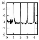
(a) Method A

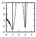
(b) Method B

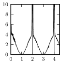
(c) Method C

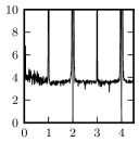
(d) Method D

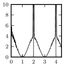
(e) Method E

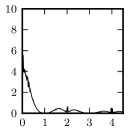
(f) Method G

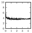
(g) IMEX Method

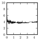
(h) Reference

Fig. 1: Maximum deviation of scaled oscillatory energy $\omega I$ on the time interval $[0,1000]$ vs. $h\omega/\pi$ ($h=0.02$).

Figure 1 depicts the maximum deviation in frequency-scaled oscillatory energy $\omega I$, over the time interval $[0,1000]$, for a range of different frequencies. As discussed in Section 1.4, deviations in $I$ are $\mathcal{O}(\omega^{-1})$, whereas those in $\omega I$ are $\mathcal{O}(1)$, making the latter more appropriate for comparison across frequencies. (To our knowledge, the use of $\omega I$ rather than $I$ for numerical experiments originated in O’Neale and McLachlan [14].) The time step size is fixed at $h=0.02$, while $h\omega/\pi$ ranges over $(0,4.5]$.

The “spikes” seen at nonzero integer values of $h\omega/\pi$ correspond to resonance instability. Note that the energy blowup is particularly severe for Method B (the Deuflhard/impulse method), while Methods C and E have resonances only at even values of $h\omega/\pi$. Only Method G and the IMEX method display no resonance spikes at all.

Away from the resonance instabilities, the energy deviation behavior is also interesting. For all of the methods considered, $\omega I$ appears to be $\mathcal{O}(1)$ away from the resonance spikes. Indeed, as long as the methods are stable (i.e., the solutions remain bounded), we have $I=\mathcal{O}(\omega^{-1})$, so all of the methods nearly conserve the adiabatic invariant $I$. (This holds true whether or not the method is consistent for the individual oscillatory energies $I_{j}$.)

However, the methods behave quite differently with respect to the magnitude of the deviations in oscillatory energy. For the reference solution, the maximum deviation in $\omega I$ is nearly constant with respect to $\omega$, with an approximate numerical value of $4$. Methods B, C, and E display a significant decrease in oscillatory energy deviation near odd integer values of $h\omega/\pi$, indicating that the adiabatic invariant is conserved too well, compared to the reference solution. (This artificial “anti-resonance” can be seen as a sort of numerical damping.) This behavior is even more dramatic for Method G, where the energy deviation is artificially low for nearly all values of $h\omega/\pi$, not just values close to odd integers. Of the methods considered, the IMEX method is the only one which correctly captures the magnitude of these deviations in oscillatory energy. This phenomenon will be revisited and analyzed in Section 4, where we will show that this behavior is governed by higher-order terms in the modulated Fourier expansion.

3.3 Long-time near-conservation of total energy

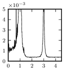
(a) Method A

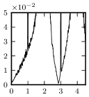
(b) Method B

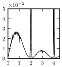
(c) Method C

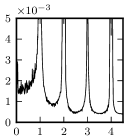
(d) Method D

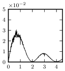
(e) Method E

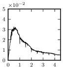
(f) Method G

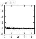
(g) IMEX Method

(h) IMEX Method

Fig. 2: Maximum deviation of total energy on the time interval $[0,1000]$ vs. $h\omega/\pi$ ($h=0.02$). The $y$-axis is scaled 10 times smaller for Methods A, D, and IMEX due to the smaller energy deviations for these methods.

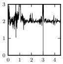
(a) Method A

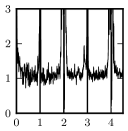
(b) Method B

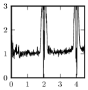
(c) Method C

(d) Method D

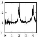
(e) Method E

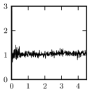
(f) Method G

(g) IMEX Method

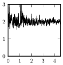
(h) IMEX Method

Fig. 3: Log ratio of the maximum deviations in total energy on the the time interval $[0,1000]$, for $h=0.02$ and $h=0.04$, plotted against $h\omega/\pi$. Away from resonances, Methods A, D and IMEX conserve total energy up to $\mathcal{O}(h^{2})$, while the remaining trigonometric integrators only conserve total energy up to $\mathcal{O}(h)$.

Figure 2 shows the maximum deviation in total energy (i.e., in the Hamiltonian), over the time interval $[0,1000]$, for a range of different frequencies. (This is in contrast to Figure 1, which depicted only the oscillatory energy component of the Hamiltonian.) The reference plot is omitted, as the exact solution preserves total energy exactly. As in Figure 1, Methods A–D again exhibit “spikes” in the energy error at resonant frequencies. Notably, this is not the case for Method E—despite the fact that it exhibited resonance spikes for the oscillatory energy alone—nor for Method G or IMEX. Furthermore, observe that Methods A, D, and IMEX conserve energy much more closely than the other methods (at least away from resonances), by roughly an order of magnitude. This is consistent with the discussion in Section 2.4, including the result in Theorem 2, which stated that these methods conserve total energy up to $\mathcal{O}(h^{2})$, whereas the remaining methods only do so up to $\mathcal{O}(h)$.

Figure 3 illustrates the relationship of total energy conservation to step size, plotting the log ratio of the deviation in total energy for $h=0.02$ and $h=0.04$. As anticipated by the theoretical results in Section 2.4, including Theorem 2, we see that the energy deviations are $\mathcal{O}(h^{2})$ for Methods A, D, and IMEX, and $\mathcal{O}(h)$ for the remaining methods (at least away from resonances). Only the IMEX method exhibits second-order conservation of total energy, while also remaining free of resonance spikes.

3.4 Slow energy exchange

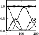
(a) Method A

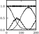
(b) Method B

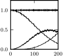
(c) Method C

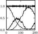
(d) Method D

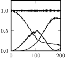
(e) Method E

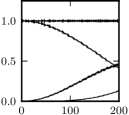
(f) Method G

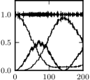
(g) IMEX Method

(h) Reference

Fig. 4: Slow exchange of individual and total oscillatory energies vs. time ($\omega=50$, $h=0.03$).

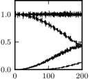
(a) Method A

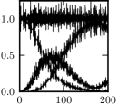
(b) Method B

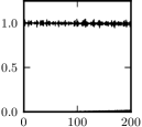
(c) Method C

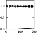
(d) Method D

(e) Method E

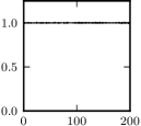
(f) Method G

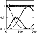
(g) IMEX Method

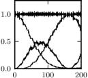
(h) Reference

Fig. 5: Slow exchange of individual and total oscillatory energies vs. time ($\omega=50$, $h=0.1$).

(a) Method A

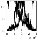
(b) Method B

(c) Method C

(d) Method D

(e) Method E

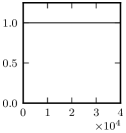
(f) Method G

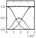
(g) IMEX Method

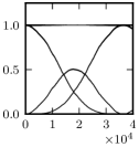
(h) Reference

Fig. 6: Slow exchange of individual and total oscillatory energies vs. time ($\omega=10000$, $h=0.1$).

Figures 4, 5, and 6 depict the phenomenon of slow energy exchange for the FPU problem, following similar numerical experiments in Hairer et al. [10]. Each plot contains four curves, corresponding to the three stiff energies, $I_{1},I_{2},I_{3}$, along with the adiabatic invariant $I=I_{1}+I_{2}+I_{3}\approx 1$.

In Figure 4, the parameters $\omega=50$ and $h=0.03$ correspond to a moderate choice of time step size: since $h\omega/\pi\approx 0.48$, this is prior to the onset of resonance instability at nonzero integer values. Methods B, D, and the IMEX method give qualitatively correct energy exchange behavior on the time interval $[0,200]$. By contrast, the exchange occurs too quickly for Method A, and too slowly for Methods C, E, and G (the latter quite dramatically).

In Figure 5, the fast frequency remains $\omega=50$, but we take a significantly larger time step size of $h=0.1$ (with $h\omega/\pi\approx 1.59$). Method B and the IMEX method still capture the correct rate of energy exchange on the time interval $[0,200]$, while for the other methods, the exchange occurs much too slowly. Notice that we are also beginning to see the effects of oscillatory energy deviation, as in Figure 1. Indeed, the excessive “noise” visible for Method B is due to the wide resonance band at $h\omega/\pi=2$, while the pronounced lack of noise in Method G is due to its artificially low deviations in oscillatory energy. Only the IMEX method displays the correct oscillatory energy behavior, capturing both the rate of exchange and the magnitude of deviations.

Next, in Figure 6, we depict the behavior of these methods as they approach their high-frequency limit, keeping $h=0.1$ but taking $\omega=10000$ (hence $h\omega/\pi\approx 318$). Since $\omega$ has been scaled by a factor of $200$ compared to the previous experiments, the time interval must also be scaled correspondingly, so we look at energy exchange over the interval $[0,40000]$. As before, only Method B and the IMEX method capture the correct rate of exchange, while for the other methods, the exchange occurs so slowly that it cannot be seen at all on the time scale considered. Method B is again hampered by resonance instability, as in Figure 5, which manifests as excess noise in the oscillatory energy plot. Of the methods considered, only the IMEX method captures the correct energy behavior in the high-frequency limit.

3.5 Global error in slow components

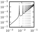
(a) Method A

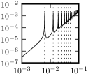
(b) Method B

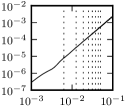
(c) Method C

(d) Method D

(e) Method E

(f) Method G

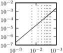
(g) IMEX Method

(h) Störmer/Verlet

Fig. 7: Global error in the slow position $x_{0}$ at the first time step after $t=1$ vs. time step size ($\omega=1000$).

(a) Method A

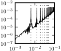
(b) Method B

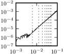
(c) Method C

(d) Method D

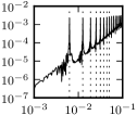
(e) Method E

(f) Method G

(g) IMEX Method

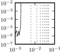
(h) Störmer/Verlet

Fig. 8: Global error in the slow momentum $y_{0}$ at the first time step after $t=1$ vs. time step size ($\omega=1000$).

Finally, in Figures 7 and 8, we investigate the global error in the slow position $x_{0}$ and slow momentum $y_{0}$, plotted against the time step size $h$. (These are the only components of real concern: indeed, trigonometric methods are designed precisely for problems where we are not interested in resolving the fast oscillations.) For both figures, the error plotted is the Euclidean distance between the numerical solution and a reference solution, taken at the first time step after $t=1$. Dotted vertical lines indicate values for which $h\omega$ is an integer multiple of $2\pi$, where some of the methods suffer from resonance instabilities that manifest as spikes in the global error. Note that the Störmer/Verlet blows up due to linear instability near $h=2/\omega=2\times 10^{-3}$, illustrating its unsuitability for this type of highly oscillatory problem.

Using the modulated Fourier expansion, the analysis of Hairer et al. [10, Chapter XIII, Theorem 4.1] shows that each of the trigonometric methods is second-order, as long as $h\omega$ is bounded away from an integer multiple of $\pi$. However, near these resonance points, the order of accuracy reduces to one unless the filter functions satisfy certain conditions. (See also Grimm and Hochbruck [8].) Among the standard trigonometric integrators, Methods C, D, and G satisfy these conditions, and hence are second-order uniformly in $h\omega$. By contrast, Methods A, B, and E do not satisfy these conditions, and the resulting error spikes (visible in Figures 7 and 8) lead to a reduction in their uniform order of accuracy.

By construction, however, the IMEX method always has $h\widetilde{\omega}$ bounded away from nonzero integer multiples of $\pi$. Indeed, since $h\widetilde{\omega}=2\arctan(\frac{1}{2}h\omega)$, we have $-\pi<h\widetilde{\omega}<\pi$, and $h\widetilde{\omega}$ approaches $\pm\pi$ only in the limit as $h\omega$ approaches $\pm\infty$. It follows that $h\widetilde{\omega}$ is bounded away from nonzero integer multiples of $\pi$ whenever $h\omega$ is bounded. Hence, comparing the modulated Fourier coefficients, the argument of Hairer et al. [10] implies that the global error in the slow components for the IMEX method is second-order, uniformly in $h\omega$ on any bounded region $\lvert h\omega\rvert\leq M$.

Combined with the previous results, we remark that only Method G and the IMEX method are uniformly second-order and free of resonance instabilities. Of these two methods, however, only IMEX captures the correct stiff energy behavior.

4 Analysis of oscillatory energy deviations

We observed in Section 3.2 that the oscillatory energy $I(x,\dot{x})$ is nearly conserved, for long times, by all the methods considered. This is proved in Hairer et al. [10, Chapter XIII, Theorem 7.1], where it is shown that the deviations in oscillatory energy are $\mathcal{O}(h)$. However, from Figure 1, it is also apparent that the magnitude of these deviations, for certain methods, is very different from the correct value displayed in the reference solution. This can be explained by carrying the modulated Fourier expansion to one more term.

For the exact solution, the system of modulated Fourier coefficients is known to have a formal invariant $\mathcal{I}=-i\omega(\overline{u}^{T}\dot{u}-u^{T}\dot{\overline{u}})+\mathcal{O}(\omega^{-6})$, where $u=e^{i\omega t}z$. A higher-order expansion of this invariant appears in [10, Chapter XIII, Equation 6.12], and the $\mathcal{O}(\omega^{-6})$ estimate is obtained by observing from [10, Chapter XIII, Equation 5.3] that the remainder is a product of $-i\omega$ with two additional factors, which are respectively $\mathcal{O}(\omega^{-4})$ and $\mathcal{O}(\omega^{-3})$. Now, with $\dot{u}=e^{i\omega t}(\dot{z}+i\omega z)=i\omega e^{i\omega t}z+\mathcal{O}(\omega^{-2})$, this gives

$$\mathcal{I}=2\omega^{2}\lVert z_{1}\rVert^{2}+\mathcal{O}(\omega^{-2}).$$

This should be compared to the oscillatory energy, which is

$$I(x,\dot{x})=\frac{1}{2}\lVert\dot{x}_{1}\rVert^{2}+\frac{1}{2}\omega^{2}\lVert x_{1}\rVert^{2}.$$

To do this, consider the expansions

$$x_{1} =y_{1}+e^{i\omega t}z_{1}+e^{-i\omega t}\overline{z}_{1}+\mathcal{O}(\omega^{-4})$$

$$\dot{x}_{1} =\dot{y}_{1}+e^{i\omega t}(z_{1}+i\omega z_{1})+e^{-i\omega t}(\overline{z}_{1}-i\omega\overline{z}_{1})+\mathcal{O}(\omega^{-4}).$$

Inserting $y_{1}=\mathcal{O}(\omega^{-2})$, $z_{1}=\mathcal{O}(\omega^{-1})$, $\dot{z}_{1}=\mathcal{O}(\omega^{-2})$, we get the estimate

$$I(x,\dot{x}) =\frac{1}{2}\omega^{2}\lVert z_{1}-\dot{z}_{1}\rVert^{2}+\frac{1}{2}\omega^{2}\lVert y_{1}+e^{i\omega t}z_{1}+e^{-i\omega t}\overline{z}_{1}\rVert^{2}+\mathcal{O}(\omega^{-2})$$

$$=2\omega^{2}\bigl{(}\lVert z_{1}\rVert^{2}+y_{1}^{T}\operatorname{Re}(e^{i\omega t}z_{1})\bigr{)}+\mathcal{O}(\omega^{-4})$$

$$=\mathcal{I}+2\omega^{2}y_{1}^{T}\operatorname{Re}(e^{i\omega t}z_{1})+\mathcal{O}(\omega^{-2}).$$

Since $\mathcal{I}$ is (nearly) conserved over long times, the second term controls the $\mathcal{O}(\omega^{-1})$ deviations in the oscillatory energy $I$. This term contains two fluctuating components, corresponding to the evolution of $y_{1}=\omega^{-2}g_{1}(y)$ and $2i\omega\dot{z}_{1}=g_{1}^{\prime}(y)z=g_{1,1}(y_{0},0)z_{1}+\mathcal{O}(\omega^{-2})$. Since the latter is controlled by the formal invariant $\mathcal{I}$, it follows that

$$\lvert I-\mathcal{I}\rvert\leq\frac{\sqrt{\mathcal{I}}}{\sqrt{2}}\omega^{-1}\bigl{\lVert}g_{1,1}(y_{0},0)\bigr{\rVert}+\mathcal{O}(\omega^{-2}).$$

Repeating the above estimates for modified trigonometric integrators gives the formal invariant

$$\mathcal{I}_{h}=2\omega^{2}\lVert z_{h,1}\rVert+\mathcal{O}(\omega^{-2}),$$

for $h\rightarrow 0$, $h\omega$ fixed, which is related to $I$ by

$$I(x_{n},\dot{x}_{n})=\mathcal{I}_{h}+2\omega^{2}y_{h,1}^{T}\operatorname{Re}(e^{i\omega t}z_{h,1})+\mathcal{O}(\omega^{-2}).$$

From the modulated Fourier expansion, we have

$$y_{h,1}=\gamma\phi(h\omega)^{-1}y_{1}+\mathcal{O}(\omega^{-3}),\qquad\dot{z}_{h,1}=\alpha\dot{z}_{1}+\mathcal{O}(\omega^{-2}).$$

Thus, although the $z_{h,1}$ factor may have an incorrect evolution on the $\mathcal{O}(\omega^{-1})$ time scale if $\alpha\neq 1$, in the neighborhood of a particular solution $(y,z)$ on the $\mathcal{O}(1)$ time scale, it does not affect the deviations in $I$. Rather, these are controlled by the first factor, and are therefore correct to leading order if and only if $\gamma=\phi$, i.e., $\omega^{2}\psi(h\widetilde{\omega})=\widetilde{\omega}^{2}\operatorname{sinc}^{2}(\frac{1}{2}h\widetilde{\omega})$.

For standard trigonometric integrators, this is true for the Gautschi-type methods with $\psi(\xi)=\operatorname{sinc}^{2}(\frac{1}{2}h\omega)$, i.e., for Method A (with $\phi=1$) and Method D (with $\phi\neq 1$). The IMEX method also satisfies this consistency condition, since $\gamma=\phi=1$. For the remaining methods, the observed deviations in Figure 1 are correct up to the factor $\gamma/\phi$ calculated above. For example, Methods C and E have $\psi(\xi)=\operatorname{sinc}^{2}(\xi)$, so

$$\frac{\gamma(\xi)}{\phi(\xi)}=\frac{\operatorname{sinc}^{2}(\xi)}{\operatorname{sinc}^{2}(\tfrac{1}{2}\xi)}=\frac{\operatorname{sinc}^{2}(\tfrac{1}{2}\xi)\cos^{2}(\tfrac{1}{2}\xi)}{\operatorname{sinc}^{2}(\tfrac{1}{2}\xi)}=\cos^{2}(\tfrac{1}{2}\xi),$$

which is clearly visible, in Figure 1, as period-$2\pi$ oscillations in the magnitude of energy deviation. On the other hand, for Method G, we have the filter $\psi(\xi)=\operatorname{sinc}^{3}(\xi)$, so

$$\frac{\gamma(\xi)}{\phi(\xi)}=\frac{\operatorname{sinc}^{3}(\xi)}{\operatorname{sinc}^{2}(\tfrac{1}{2}\xi)}=\frac{\operatorname{sinc}^{3}(\tfrac{1}{2}\xi)\cos^{3}(\tfrac{1}{2}\xi)}{\operatorname{sinc}^{2}(\tfrac{1}{2}\xi)}=\operatorname{sinc}(\tfrac{1}{2}\xi)\cos^{3}(\tfrac{1}{2}\xi),$$

which leads to rapid decay in the magnitude of energy deviation.

5 Conclusion

This paper was motivated by the fact that, while conventional trigonometric integrators have many desirable properties—especially, with respect to stability, accuracy, and energy behavior—there are “no-go theorems” making it impossible for any single integrator to have these good properties simultaneously. Other work, particularly on multi-force methods, showed a way around these obstacles, but at the cost of several nonlinear force evaluations per time step. On the other hand, the observations of Stern and Grinspun [15] regarding the IMEX method suggested that, by modifying the fast frequency, one might find another way around these obstacles, without suffering the greater computational cost required by multi-force methods.

By extending the modulated Fourier expansion techniques of Hairer and Lubich [9], Hairer et al. [10], we have shown that, for modified trigonometric integrators, it is indeed possible to get around these no-go theorems—and that the IMEX method is in fact the unique modified trigonometric integrator which correctly models the multiscale phenomenon of slow energy exchange. Moreover, the IMEX method maintains desirable properties with respect to resonance stability and preservation of adiabatic invariants, while also being uniformly of second-order accuracy in global error, and does so without any additional computational cost relative to conventional trigonometric integrators. Finally, we have shown that while all of these integrators exhibit near-conservation of oscillatory energy, only some of them—in particular, the Gautschi-type trigonometric integrators and the IMEX method—consistently model the magnitude of deviations in this adiabatic invariant.

References

• Biesiadecki and Skeel [1993] J. J. Biesiadecki and R. D. Skeel, Dangers of multiple time step methods, J. Comput. Phys., 109 (1993), pp. 318–328.
• Debussche and Faou [2009] A. Debussche and E. Faou, Modified energy for split-step methods applied to the linear Schrödinger equation, SIAM J. Numer. Anal., 47 (2009), pp. 3705–3719.
• Deuflhard [1979] P. Deuflhard, A study of extrapolation methods based on multistep schemes without parasitic solutions, Z. Angew. Math. Phys., 30 (1979), pp. 177–189.
• Fermi et al. [1955] E. Fermi, J. Pasta, and S. Ulam, Studies of nonlinear problems, Report LA-1940, Los Alamos National Laboratory, Los Alamos, NM, 1955.
• Galgani et al. [1992] L. Galgani, A. Giorgilli, A. Martinoli, and S. Vanzini, On the problem of energy equipartition for large systems of the Fermi-Pasta-Ulam type: analytical and numerical estimates, Phys. D, 59 (1992), pp. 334–348.
• García-Archilla et al. [1999] B. García-Archilla, J. M. Sanz-Serna, and R. D. Skeel, Long-time-step methods for oscillatory differential equations, SIAM J. Sci. Comput., 20 (1999), pp. 930–963 (electronic).
• Gautschi [1961] W. Gautschi, Numerical integration of ordinary differential equations based on trigonometric polynomials, Numer. Math., 3 (1961), pp. 381–397.
• Grimm and Hochbruck [2006] V. Grimm and M. Hochbruck, Error analysis of exponential integrators for oscillatory second-order differential equations, J. Phys. A, 39 (2006), pp. 5495–5507.
• Hairer and Lubich [2000] E. Hairer and C. Lubich, Long-time energy conservation of numerical methods for oscillatory differential equations, SIAM J. Numer. Anal., 38 (2000), pp. 414–441 (electronic).
• Hairer et al. [2006] E. Hairer, C. Lubich, and G. Wanner, Geometric numerical integration, vol. 31 of Springer Series in Computational Mathematics, Springer-Verlag, Berlin, second ed., 2006. Structure-preserving algorithms for ordinary differential equations.
• Hochbruck and Lubich [1999] M. Hochbruck and C. Lubich, A Gautschi-type method for oscillatory second-order differential equations, Numer. Math., 83 (1999), pp. 403–426.
• Leimkuhler and Reich [2004] B. Leimkuhler and S. Reich, Simulating Hamiltonian dynamics, vol. 14 of Cambridge Monographs on Applied and Computational Mathematics, Cambridge University Press, Cambridge, 2004.
• McLachlan and Quispel [2002] R. I. McLachlan and G. R. W. Quispel, Splitting methods, Acta Numer., 11 (2002), pp. 341–434.
• O’Neale and McLachlan [2009] D. R. J. O’Neale and R. I. McLachlan, Reconsidering trigonometric integrators, ANZIAM J., 50 (2009), pp. 320–332.
• Stern and Grinspun [2009] A. Stern and E. Grinspun, Implicit-explicit variational integration of highly oscillatory problems, Multiscale Model. Simul., 7 (2009), pp. 1779–1794.
• Zhang and Skeel [1997] M. Zhang and R. D. Skeel, Cheap implicit symplectic integrators, Appl. Numer. Math., 25 (1997), pp. 297–302. Special issue on time integration.