Determination of $S$-curves with applications to the theory of nonhermitian orthogonal polynomials

Abstract

This paper deals with the determination of the $S$-curves in the theory of non-hermitian orthogonal polynomials with respect to exponential weights along suitable paths in the complex plane. It is known that the corresponding complex equilibrium potential can be written as a combination of Abelian integrals on a suitable Riemann surface whose branch points can be taken as the main parameters of the problem. Equations for these branch points can be written in terms of periods of Abelian differentials and are known in several equivalent forms. We select one of these forms and use a combination of analytic an numerical methods to investigate the phase structure of asymptotic zero densities of orthogonal polynomials and of asymptotic eigenvalue densities of random matrix models. As an application we give a complete description of the phases and critical processes of the standard cubic model.

1 Introduction

The present paper elaborates on the notion of $S$-curve of Stahl [1, 2, 3, 4] and of Gonchar and Rakhmanov [5, 6]. Among the many applications of $S$-curves (see for instance section 6.3 of [7] and references therein), we pay special attention to the theory of nonhermitian orthogonal polynomials $p_{n}(z)=z^{n}+\cdots$

$$\int_{\Gamma}p_{n}(z)z^{k}\rme^{-nW(z)}\rmd z=0,\quad k=0,\ldots,n-1.$$ (1)

The classical theory of orthogonal polynomials corresponds to the hermitian case, in which the integration path $\Gamma$ is typically a real interval and the weight is a positive real function on $\Gamma$. But more recently the nonhermitian case, in which $\Gamma$ can be a more general curve in the complex plane and the weight can be a complex function, has received much attention. In the mathematical literature these polynomials first appeared as denominators of Padé and other types of rational approximants [1, 2, 3, 4], but the corresponding theory quickly developed and found applications into such fields as the Riemann-Hilbert approach to strong asymptotics, random matrix theory [8, 9, 10, 11, 12, 13] and, consequently, in the study of dualities between supersymmetric gauge theories and string models [14, 15, 16, 17, 18].

More concretely, our aim is to apply the general theory of $S$-curves as developed in [5, 6, 7] to study the asymptotic distribution of zeros of orthogonal polynomials and the phase structure of the asymptotic distribution of eigenvalues as $n\rightarrow\infty$ of random matrix problems of the form [19, 20, 21, 22, 23]

$$Z_{n}=\int\rmd M\rme^{-n{\rm Tr}W(M)},$$ (2)

where the eigenvalues of the $n\times n$ matrices $M$ are constrained to lie on $\Gamma$.

Throughout our discussion we assume that $W(z)$ is a complex polynomial and $\Gamma$ is a simple analytic curve connecting two different convergence sectors ($\mathop{\rm Re}\nolimits W(z)>0$) at infinity of (1). A fundamental result of Gonchar and Rakhmanov [5] asserts that if $\Gamma$ is an $S$-curve, then the asymptotic zero distribution of $p_{n}(z)$ exists and is given by the equilibrium charge density [24] that minimizes the electrostatic energy (among normalized charge densities supported on the curve $\Gamma$) in the presence of the external electrostatic potential $V(z)=\mathop{\rm Re}\nolimits W(z)$. Note that the integral (1) is invariant under deformations of the curve $\Gamma$ into curves in the same homology class and connecting the same two convergence sectors at infinity. This freedom to deform $\Gamma$ means that only for special choices of $\Gamma$ the asymptotic zero distribution has support on $\Gamma$. According to recent results by Rakhmanov [6], given a family of orthogonal polynomials of the form (1) we can always deform $\Gamma$ into an appropriate $S$-curve.

We use an analytic scheme, to be implemented in general with the help of numerical analysis, based on the study of certain algebraic curves which arise as a direct consequence of the $S$-property [5, 6, 7]. These spectral curves have the form

$$y^{2}=W^{\prime}(z)^{2}+f(z),$$ (3)

where $f(z)$ is a polynomial such that $\deg f=\deg W-2$. The main parameters that determine the $S$-curves and the associated equilibrium densities are the branch points of $y(z)$, which turn out to be the endpoints of the (in general, several disjoint) arcs (cuts) that support the equilibrium density. Systems of equations for these branch points can be formulated in terms of period integrals of $y(z)$ and are known in several equivalent forms. We select one of these forms that in the Hermitian case reduces to the system of equations derived in [25]. The corresponding cuts are characterized as Stokes lines of the polynomial $y(z)^{2}$ or, equivalently, as trajectories of the quadratic differential $y(z)^{2}(\rmd z)^{2}$. At this point we use numerical analysis not only to solve the equations for the cut endpoints but also to analyze the existence of cuts satisfying the $S$-property.

Recently Bertola and Mo [12] and Bertola [13] have used the notion of Boutroux curves to characterize the support of the asymptotic distribution of zeros of families of nonhermitian orthogonal polynomials. Both the calculations of the present paper and the approach of [12, 13] do not rely on the minimization of a functional but on the characterization of spectral curves (3) with appropriate cuts. This characterization is formulated in [12, 13] in terms of admissible Boutroux curves which are determined from certain combinatorial and metric data in the space of polynomials $p(z)$. It can be proved that the branch cut structure of admissible Boutroux curves consists of arcs satisfying the $S$-property and, consequently, the method of [12, 13] can also be applied to characterize $S$-curves. However, as we explained in the previous paragraph, our calculations are based on an explicit system of equations for the cut endpoints. In contrast, the generation of nontrivial explicit examples in [12, 13] amounts to imposing directly period conditions by means of a numerical algorithm involving the minimization of a functional that vanishes precisely for admissible Boutroux curves.

The paper is organized as follows. In section 2 we review the basic results on equilibrium densities of electrostatic models under the action of external fields. Then we introduce the notions of $S$-curve and $S$-property, and discuss their relevance to characterize asymptotic zero densities of orthogonal polynomials. To obtain an equivalent but computationally more efficient formulation of the $S$-property it is convenient to introduce the complex counterpart of the electrostatic potential. This formulation leads naturally to the notion of spectral curve. In section 3 we recall the theoretical background to construct equilibrium densities on $S$-curves for a given polynomial $W(z)$ and use the theory of Abelian differentials in Riemann surfaces to derive a system of equations for the cut endpoints. We also discuss the characterization of cuts as Stokes lines and the process of embedding the cuts into $S$-curves. In section 4 we apply the former results to perform a complete analysis of the cubic model

$$W(z)=\frac{z}{3}-tz,$$ (4)

with a varying complex coefficient $t$. We determine $S$-curves and equilibrium densities for the two possible cases corresponding to equilibrium densities supported on one or two disjoint arcs. Our analysis combines theoretical properties with numerical calculations and allows us to characterize critical processes of merging, splitting, birth and death at a distance of cuts. As a consequence we describe the phase structure of the corresponding families of orthogonal polynomials on different paths $\Gamma$. The consistency of our results is checked by superimposing the cuts and the zeros of the corresponding orthogonal polynomials $p_{n}(z)$ with degree $n=24$. Thus we find a complete agreement with the Gonchar-Rakhmanov Theorem [5] (Theorem 1 below). Finally, in section 5 we briefly discuss a generalization of the $S$-property which arises in the study of dualities between supersymmetric gauge theories and string models on local Calabi-Yau manifolds. Some technical aspects of the theoretical discussion are treated in appendix A.

2 Zero densities of orthogonal polynomials

According to the general theory of logarithmic potentials with external fields [24], given an analytic curve $\Gamma$ in the complex plane and a real-valued external potential $V(z)$, there exists a unique charge density $\rho(z)$ that minimizes the total electrostatic energy

$$\mathcal{E}[\rho]=\int_{\Gamma}|\rmd z|\rho(z)V(z)-\int_{\Gamma}|\rmd z|\int_{\Gamma}|\rmd z^{\prime}|\log|z-z^{\prime}|\rho(z)\rho(z^{\prime})$$ (5)

among all positive densities supported on $\Gamma$ such that

$$\int_{\Gamma}|\rmd z|\rho(z)=1.$$ (6)

This density $\rho(z)$ is called the equilibrium density, and its support $\gamma$ is a finite union of disjoint analytic arcs $\gamma_{i}$ (cuts) contained in $\Gamma$:

$$\gamma=\gamma_{1}\cup\gamma_{2}\cup\cdots\cup\gamma_{s}\subset\Gamma.$$ (7)

In terms of the total electrostatic potential

$$U(z)=V(z)-2\int_{\Gamma}|\rmd z^{\prime}|\rho(z^{\prime})\log|z-z^{\prime}|,$$ (8)

the equilibrium density is characterized by the existence of a real constant $l$ such that

$$U(z)=l,\quad z\in\gamma,$$ (9)

$$U(z)\geq l,\quad z\in\Gamma-\gamma.$$ (10)

The property that relates this minimization problem to the asymptotic zero density of orthogonal polynomials is called the S-property, and was singled out by Stahl [1, 2, 3, 4], elaborated by Gonchar and Rakhmanov [26, 5], and more recently extended by Martínez-Finkelshtein and Rakhmanov [7].

A curve $\Gamma$ is said to be an $S$-curve with respect to the external field $V(z)$ if for every interior point $z$ of the support $\gamma$ of the equilibrium density the total potential (8) satisfies

$$\frac{\partial U(z)}{\partial n_{+}}=\frac{\partial U(z)}{\partial n_{-}},$$ (11)

where $n_{\pm}$ denote the two normal vectors to $\gamma$ at $z$ pointing in the opposite directions. In this case it is said that $\gamma$ satisfies the $S$-property. The condition (11) means that the electric fields at each side are opposite, $\mathbf{E}_{+}=-\mathbf{E}_{-}$.

2.1 Orthogonal polynomials and $S$-curves

Let $\{p_{n}(z)\}_{n\geq 1}$ be a family of monic orthogonal polynomials on a curve $\Gamma$ with respect to an exponential weight $\exp(-nW(z))$,

$$\int_{\Gamma}p_{n}(z)z^{k}\rme^{-nW(z)}\rmd z=0,\quad k=0,\ldots,n-1.$$ (12)

Here and henceforth we assume that $W(z)$ is a complex polynomial of degree $N+1$

$$W(z)=\sum_{k=1}^{N+1}t_{k}\,z^{k},$$ (13)

and that $\Gamma$ is an oriented simple analytic curve which as $z\rightarrow\infty$ connects two different sectors of convergence of (12). The notion of $S$-curve is crucial in the analysis of the limit as $n\rightarrow\infty$ of the zero density $\frac{1}{n}(\delta(z-c_{1})+\cdots+\delta(z-c_{n}))$ of $p_{n}(z)$. The following Theorem (see [5], section 3) states the close relation between the asymptotic zero distribution of orthogonal polynomials and the equilibrium densities on $S$-curves:

Theorem 1

Let $\{p_{n}(z)\}_{n\geq 1}$ be a family of orthogonal polynomials on a curve $\Gamma$ with respect to an exponential weight $\exp(-nW(z))$. If $\Gamma$ is an $S$-curve with respect to the external potential $V(z)=\mathop{\rm Re}\nolimits W(z)$, then the equilibrium density on $\Gamma$ is the weak limit as $n\rightarrow\infty$ of the zero density of $p_{n}(z)$.

It often occurs in the applications that the orthogonal polynomials $p_{n}(z)$ are initially defined on a curve $\Gamma$ which is not an $S$-curve. This problem raises the question of the existence of an $S$-curve in the same homology class of $\Gamma$ connecting the same pair of convergence sectors at infinity (and therefore defining the same family of orthogonal polynomials). This question has been recently solved in the affirmative by Rakhmanov (see [6], section 5.3). Note also that although this $S$-curve is not unique, the associated equilibrium density is certainly unique.

2.2 Matrix models

Equilibrium densities on $S$-curves are also expected to describe the asymptotic eigenvalue distribution as $n\rightarrow\infty$ of random matrix models with partition function (2). According to Heine’s formula [21], the polynomials (1) are the expectation values of the characteristic polynomials of the matrices $M$ of the ensemble,

$$p_{n}(z)=\frac{1}{Z_{n}}\int\rmd M\det(z-M)\rme^{-n\mathop{\rm Tr}\nolimits W(M)}.$$ (14)

In terms of the zeros $\{c_{i}\}_{i=1}^{n}$ of $p_{n}(z)$ and of the eigenvalues $\{\lambda_{i}\}_{i=1}^{n}$ of $M$, this result means that the expectation value of the function $\prod_{i=1}^{n}(z-\lambda_{i})$ is the function $\prod_{i=1}^{n}(z-c_{i})$. Therefore it is natural to conjecture that the asymptotic distributions of zeros of $p_{n}(z)$ and of eigenvalues of $M$ coincide. This conjecture has been rigorously proved in the hermitian case, i.e., when $\Gamma=\mathbb{R}$ and the polynomial $W(z)$ has real coefficients [8, 21], and indeed orthogonal polynomials are a widely used tool in many aspects of hermitian random matrix theory (for some recent applications see [27, 28]).

2.3 Spectral curves

The $S$-property can be formulated in a more convenient form to our goals using a complex counterpart of the electrostatic potential (8). Thus, we define

$$\mathcal{U}(z)=W(z)-(g(z_{+})+g(z_{-})),$$ (15)

where $g(z)$ is the analytic function in $\mathbb{C}\setminus\Gamma$ given by

$$g(z)=\int_{\gamma}|\rmd z^{\prime}|\rho(z^{\prime})\log(z-z^{\prime}).$$ (16)

Here we assume that the logarithmic branch is taken in such a way that for every $z^{\prime}\in\Gamma$ the function $\log(z-z^{\prime})$ is an analytic function of $z$ in $\mathbb{C}$ minus the semi-infinite arc of $\Gamma$ ending at $z^{\prime}$. As usual $g(z_{+})$ and $g(z_{-})$ denote the limits of the function $g(z^{\prime})$ as $z^{\prime}$ tends to $z$ from the left and from the right of the oriented curve $\Gamma$ respectively.

It is clear that

$$\mathop{\rm Re}\nolimits\mathcal{U}(z)=U(z),$$ (17)

and therefore the equilibrium condition (9) can be rewritten as

$$\mathop{\rm Re}\nolimits\mathcal{U}(z)=l,\quad z\in\gamma.$$ (18)

Furthermore, it follows from the Cauchy-Riemann equations that the $S$-property (11) is verified if and only if the imaginary part of $\mathcal{U}(z)$ is constant on each arc $\gamma_{j}$ of $\gamma$ (usually stated as “locally constant on $\gamma$”) [7, 29]:

$$\mathop{\rm Im}\nolimits\mathcal{U}(z)=m_{j},\quad z\in\gamma_{j},\quad j=1,\ldots,s.$$ (19)

Note that, in essence, the $S$-property embodies the possibility of analytically continuing the derivative of the complex equilibrium potential through the support. In some physical applications [14, 30, 31] the values $L_{j}=l+\rmi m_{j}$ are especially relevant, and equations (18) and (19) are (trivially) restated by saying that $\Gamma$ is an $S$-curve if and only if the complex potential $\mathcal{U}(z)$ is locally constant on $\gamma$

$$\mathcal{U}(z)=L_{j},\quad z\in\gamma_{j},\quad j=1,\ldots,s,$$ (20)

and the constants $L_{j}$ have the same real part

$$\mathop{\rm Re}\nolimits L_{1}=\cdots=\mathop{\rm Re}\nolimits L_{s}.$$ (21)

Next we will see how equations (20) lead to the notion of spectral curve. (In section 3.1 we will see that equations (21) are essential to formulate the system of equations for the cut endpoints in the multicut case.) In fact, condition (20) can be rewritten in a form especially suited for practical applications in terms of a new function $y(z)$ defined by

$$y(z)=W^{\prime}(z)-2g^{\prime}(z)=W^{\prime}(z)-2\int_{\gamma}|\rmd z^{\prime}|\frac{\rho(z^{\prime})}{z-z^{\prime}},\quad z\in\mathbb{C}\setminus\Gamma.$$ (22)

Proposition 1

The complex potential $\mathcal{U}(z)$ is locally constant on $\gamma$ if and only if the square of $y(z)$ is a polynomial of the form

$$y(z)^{2}=W^{\prime}(z)^{2}+f(z),$$ (23)

where $f(z)$ is a polynomial of degree $\deg f=\deg W-2$.

Proof. Condition (20) is equivalent to

$$W^{\prime}(z)-(g^{\prime}(z_{+})+g^{\prime}(z_{-}))=0,\quad z\in\gamma,$$ (24)

where

$$g^{\prime}(z)=\int_{\gamma}|\rmd z^{\prime}|\frac{\rho(z^{\prime})}{z-z^{\prime}},$$ (25)

and therefore (24) can be written as

$$y(z_{+})=-y(z_{-}),\quad z\in\gamma.$$ (26)

The function $y(z)$ is analytic in $\mathbb{C}\setminus\gamma$ and, due to (26), its square is continuous on $\gamma$. Hence $y^{2}(z)$ is analytic in the whole $\mathbb{C}$. Furthermore, since

$$g^{\prime}(z)=\frac{1}{z}+\mathcal{O}\left(\frac{1}{z^{2}}\right),\quad z\rightarrow\infty,$$ (27)

we have that

$$y(z)=W^{\prime}(z)-\frac{2}{z}+\mathcal{O}\left(\frac{1}{z^{2}}\right),\quad z\rightarrow\infty,$$ (28)

and Liouville’s theorem implies that $y^{2}(z)$ is a polynomial of degree $2N$ with $N=\deg W-1$. Therefore, we have

$$y^{2}=W^{\prime}(z)^{2}+f(z)$$ (29)

where

$$f(z)=y^{2}(z)-W^{\prime}(z)^{2}=4g^{\prime}(z)(g^{\prime}(z)-W^{\prime}(z))$$ (30)

is a polynomial of degree $N-1$. Reciprocally, given $\rho(z)$, if the function (22) is such that its square is a polynomial then it satisfies (26) and consequently (24).

Equation (23) defines an algebraic curve referred to as a spectral curve, which determines the equilibrium charge density via (22),

$$\rho(z)|\rmd z|=y(z_{+})\frac{\rmd z}{2\pi\rmi}=-y(z_{-})\frac{\rmd z}{2\pi\rmi},\quad z\in\gamma,$$ (31)

where $\gamma$ has the orientation inherited by the orientation of $\Gamma$.

2.4 The hermitian case

Hermitian families of orthogonal polynomials correspond to $\Gamma=\mathbb{R}$ and $W(z)$ with real coefficients. In this hermitian case it is clear that the real line $\Gamma=\mathbb{R}$ is an $S$-curve, because taking $\log(z-z^{\prime})$ as the principal branch of the logarithm we have

$$\log(z_{+}-z^{\prime})+\log(z_{-}-z^{\prime})=2\log|z-z^{\prime}|,\quad z,z^{\prime}\in\mathbb{R}.$$ (32)

Hence (19) holds because

$$\mathop{\rm Im}\nolimits\mathcal{U}(x)=\mathop{\rm Im}\nolimits\left[W(x)-\left(g(x_{+})+g(x_{-})\right)\right]=0,\quad x\in\gamma\subset\mathbb{R}.$$ (33)

There is a well stablished theory for characterizing the asymptotic distribution of zeros for hermitian orthogonal polynomials and the asymptotic distribution of eigenvalues for hermitian matrix models [8, 9, 10, 11, 21]. In particular, a method of analysis of the phase structure and critical processes for multicut hermitian matrix models was recently presented in [25].

3 Construction of equilibrium densities on $S$-curves

In this section we discuss the theoretical background underlying the determination of $S$-curves. Using Proposition 1, we begin by looking for spectral curves (23) where $\deg f=\deg W-2=N-1$. Obviously, the number $s$ of possible cuts for a fixed $W(z)$ is at most $N$. We assume for simplicity that $y^{2}(z)$ has only simple or double roots. The simple roots will be denoted by $\{a_{j}^{\pm}\}_{j=1}^{s}$ and the double roots by $\{\alpha_{l}\}_{l=1}^{r}$. The simple roots $a_{j}^{\pm}$ will be the endpoints of the cut $\gamma_{j}$, and therefore $r+s=N$.

To determine the branch of $y(z)$ that verifies (28) in the $s$-cut case, we write $y(z)$ in the form

$$y(z)=h(z)w(z),$$ (34)

$$h(z)=\prod_{l=1}^{r}(z-\alpha_{l}),\quad w(z)=\sqrt{\prod_{m=1}^{s}(z-a_{m}^{-})(z-a_{m}^{+})},$$ (35)

and take the branch of $w(z)$ such that

$$w(z)\sim z^{s},\quad z\rightarrow\infty.$$ (36)

The factor $h(z)$ in (34) is then given by

$$h(z)=\left(\frac{W^{\prime}(z)}{w(z)}\right)_{\oplus},$$ (37)

where $\oplus$ stands for the sum of the nonnegative powers of the Laurent series at infinity. Hence the function $y(z)$ is completely determined by its branch points $\{a_{j}^{\pm}\}_{j=1}^{s}$, and satisfies

$$y(z)=W^{\prime}(z)+\mathcal{O}\left(\frac{1}{z}\right),\quad z\rightarrow\infty.$$ (38)

Our first task is to find a system of equations for the cut endpoints $\{a_{j}^{\pm}\}_{j=1}^{s}$.

3.1 Equations for the cut endpoints

We use the theory of Abelian differentials in Riemann surfaces to find a system of equations satisfied by the cut endpoints (see Appendix A for definitions and notations). Let us denote by $M$ the hyperelliptic Riemann surface associated to the curve

$$w^{2}=\prod_{m=1}^{s}(z-a_{m}^{-})(z-a_{m}^{+}).$$ (39)

We introduce the meromorphic differential $\mathrm{y}(z)\rmd z$ in $M$, where $\mathrm{y}(z)$ is the extension of the function (34) to the Riemann surface $M$ in terms of two branches of $\mathrm{y}(z)$ in $M$ given by $y_{1}(z)=-y_{2}(z)=y(z)$. The asymptotic condition (28) implies

$$\mathrm{y}(z)\rmd z=\left\{\begin{array}[]{ll}\displaystyle\left(W^{\prime}(z)-\frac{2}{z}+\mathcal{O}(z^{-2})\right)\rmd z,\quad\mbox{as $z\rightarrow\infty_{1}$},\\ \displaystyle\left(-W^{\prime}(z)+\frac{2}{z}+\mathcal{O}(z^{-2})\right)\rmd z,\quad\mbox{as $z\rightarrow\infty_{2}$}.\end{array}\right.$$ (40)

Since the only poles of $\mathrm{y}(z)\rmd z$ are at $\infty_{1}$ and $\infty_{2}$, equation (40) shows that (with $t_{0}=-1$)

$$\frac{1}{2}\left(\mathrm{y}(z)+W^{\prime}(z)\right)\rmd z-\sum_{n=0}^{N+1}t_{n}\rmd\Omega_{n}$$ (41)

is a first kind Abelian differential in $M$. Hence it admits a decomposition in the canonical basis

$$\frac{1}{2}\left(\mathrm{y}(z)+W^{\prime}(z)\right)\rmd z-\sum_{n=0}^{N+1}t_{n}\rmd\Omega_{n}=\sum_{j=1}^{s-1}\lambda_{j}\rmd\varphi_{j},$$ (42)

for some complex coefficients $\lambda_{j}\in\mathbb{C}$. Thus, we may write

$$\mathrm{y}(z)\rmd z=-W^{\prime}(z)\rmd z+2\sum_{j=1}^{s-1}\lambda_{j}\rmd\varphi_{j}+2\sum_{n=0}^{N+1}t_{n}\rmd\Omega_{n}.$$ (43)

Let us now denote by $\gamma_{j}$ a set of oriented cuts joining the pairs $a_{j}^{-}$ and $a_{j}^{+}$ of the function (34), and by $z_{j}$ an arbitrary point in $\gamma_{j}$. The $A$-periods of the differential $\mathrm{y}(z)\rmd z$ can be written as

$$A_{j}(\mathrm{y}(z)\rmd z)=\int_{z_{j}+}^{z_{(j+1)}+}y_{1}(z)\rmd z+\int_{z_{(j+1)}-}^{z_{j}-}y_{2}(z)\rmd z.$$ (44)

Since $y_{1}(z)=-y_{2}(z)=y(z)$, we have that $y_{2}(z_{-})=-y_{2}(z_{+})=y_{1}(z_{+})=-y_{1}(z_{-})$. Hence from (22) and (21) we get

$$A_{j}(\mathrm{y}(z)\rmd z)=2\left[W(z_{j+1})-\left(g(z_{(j+1)+})+g(z_{(j+1)-})\right)\right]-2\left[W(z_{j})-\left(g(z_{j+})+g(z_{j-})\right)\right]$$

$$=2(L_{j+1}-L_{j})=2\rmi(m_{j+1}-m_{j})\in\rmi\mathbb{R}.$$ (45)

As a consequence, the coefficients $\lambda_{j}$ in (43) are given by

$$\lambda_{j}=\rmi r_{j},\quad r_{j}=m_{j+1}-m_{j}\in\mathbb{R}.$$ (46)

Furthermore, from (31) we find that the $B$-periods are

$$B_{i}(\mathrm{y}(z)\rmd z)=-4\pi\rmi\sum_{j=1}^{i}\int_{\gamma_{j}}|\rmd z|\rho(z)\in\rmi\mathbb{R},$$ (47)

and consequently (43) implies

$$\sum_{j=1}^{s-1}r_{j}\mathop{\rm Im}\nolimits B_{i}(\rmd\varphi_{j})=\mathop{\rm Re}\nolimits\left(\sum_{n=0}^{N+1}t_{n}B_{i}(\rmd\Omega_{n})\right).$$ (48)

Since the matrix of periods $\mathop{\rm Im}\nolimits B_{i}(\rmd\varphi_{j})$ is positive definite [32], the linear system (48) uniquely determines the coefficients $r_{j}$ as functions of the cut endpoints $\{a_{k}^{\pm}\}_{k=1}^{s}$ and the coefficients $\{t_{n}\}_{n=1}^{N+1}$ of the potential $W(z)$.

Therefore, we have the following method to find a system of equations for the cut endpoints:

(1)

We start with a function $y(z)$ of the form (34)–(35) and use the identity

$$\prod_{l=1}^{r}(z-\alpha_{l})=\left(\frac{W^{\prime}(z)}{w(z)}\right)_{\oplus}$$ (49)

to determine the double roots $\{\alpha_{l}\}_{l=1}^{r}$ of $y^{2}(z)$ in terms of the cut endpoints. Then we express the coefficients of the polynomial $y(z)^{2}-W^{\prime}(z)^{2}$ in terms of the cut endpoints and the coefficients of $W(z)$.

(2)

From (34)–(37) it is clear that

$$y(z)^{2}-W^{\prime}(z)^{2} =\left(\frac{W^{\prime}(z)}{w(z)}\right)_{\ominus}\left[\left(\frac{W^{\prime}(z)}{w(z)}\right)_{\ominus}w(z)^{2}-2W^{\prime}(z)w(z)\right]$$ (50)

$$=\mathcal{O}\left(z^{N+s-1}\right),\quad z\rightarrow\infty.$$

Moreover, in order to satisfy  (30), we impose that

$$y(z)^{2}-W^{\prime}(z)^{2}=-4z^{N-1}t_{N+1}+\cdots.$$ (51)

Therefore, we equate to zero the coefficients of the powers $z^{N},\cdots,z^{N+s-1}$ and to -$4t_{N+1}$ the coefficient of $z^{N-1}$ in (50). Thus we obtain $s+1$ equations for the $2s$ cut endpoints.

(3)

Finally, to obtain $s-1$ additional equations, we express the differentials $\rmd\varphi_{j}$ and $\rmd\Omega_{n}$ in terms of the cut endpoints and solve the system (48) to determine the unknowns $r_{j}$ as functions of the cut endpoints and of the coefficients of $W(z)$. Then, in view of (43)–(46) we impose

$$\oint_{A_{i}}\mathrm{y}(z)\rmd z=2\rmi r_{i},\quad i=1,\ldots,s-1.$$ (52)

There is an alternative and more intrinsic scheme for finding the cut endpoints using the expressions of the Abelian differentials. Indeed, as a consequence of the identities (110), (112) and (115) of Appendix A we have

$$y(z)w(z)=2\sum_{n=0}^{N+1}t_{n}P_{n}(z)+2\rmi\sum_{i=1}^{s-1}r_{i}p_{i}(z).$$ (53)

Hence if we set $z=a_{j}^{\pm}$ in this identity we find

$$\sum_{n=0}^{N+1}t_{n}P_{n}(a_{j}^{\pm})+\rmi\sum_{i=1}^{s-1}r_{i}p_{i}(a_{j}^{\pm})=0,\quad j=1,\ldots,s.$$ (54)

In particular for the hermitian case (see subsection 1.3)

$$r_{i}=m_{i+1}-m_{i}=0,\quad i=1,\ldots,s-1,$$ (55)

so that (54) simplifies to

$$\sum_{n=0}^{N+1}t_{n}P_{n}(a_{j}^{\pm})=0,\quad j=1,\ldots,s,$$ (56)

which is the standard system used in hermitian random matrix models to determine the asymptotic eigenvalue support [25]. In section 4.2 we will illustrate for the usual cubic model how the new terms in the general equations (54) are reduced (via real parts and imaginary parts of periods of abelian differentials) to the calculation of standard integrals, which in this particular case can be expressed in closed form in terms of elliptic functions.

3.2 Construction of $S$-curves

Once a solution of the endpoint equations has been obtained, the $y$-function (34) is completely determined. The next step is to find the cuts $\gamma_{j}$ connecting the respective pairs of cut endpoints $a_{j}^{\pm}$ and such that the $\rho(z)$ defined by (31) is a normalized positive density and the $S$-property on $\gamma=\gamma_{1}\cup\ldots\cup\gamma_{s}$ is satisfied.

Let us define the function

$$G(z)=\int_{a_{1}^{-}}^{z}y(z^{\prime}_{+})\rmd z^{\prime}.$$ (57)

From (9) and  (22) we have that the $y$-function must satisfy

$$\mathop{\rm Re}\nolimits\int_{a_{1}^{-}}^{z}y(z^{\prime})\rmd z^{\prime} =\mathop{\rm Re}\nolimits\left[(W(z)-2g(z))-(W(a_{1}^{-})-2g(a_{1}^{-}))\right]$$ (58)

$$=U(z)-l,\quad z\in\mathbb{C}\setminus\gamma,$$

where $U(z)$ is the electrostatic potential (8) and $l$ is some real constant. Hence, in terms of $G(z)$ the equilibrium condition (9) reads

$$\mathop{\rm Re}\nolimits G(z)=0,\quad z\in\gamma.$$ (59)

Note that different choices of the base point among the branch points $a_{j}^{-}$ in the integral (57) lead to conditions equivalent to (59).

Given a root $z_{0}$ of $y^{2}(z)$ with multiplicity $m$, there are $m+2$ maximal connected components (excluding any zeros of $y^{2}(z)$) of the level curve

$$\mathop{\rm Re}\nolimits\int_{z_{0}}^{z}y(z^{\prime}_{+})\rmd z^{\prime}=0,$$ (60)

which stem from $z_{0}$ [33]. These maximal components are called the Stokes lines outgoing from $z_{0}$ associated to the polynomial $y^{2}(z)$. Stokes lines for a polynomial cannot make loops and end necessarily either at a different zero of $y(z)$ (lines of short type) or at infinity (lines of leg type). Therefore, the condition (59) means that the cuts $\gamma_{j}$ must be short type lines with cut endpoints $a_{j}^{\pm}$ of the polynomial $y^{2}(z)$. It should be noticed that the function $y(z)$ is continuous on those short type lines which are not cuts. In what follows we will denote by $\mathcal{X}_{0}$ the set of all the Stokes lines emerging from the simple roots $a_{j}^{\pm}$ of $y(z)$ and by $\mathcal{X}$ the set of all the Stokes lines emerging from all the roots of $y^{2}(z)$.

The positivity of the corresponding density (31) also imposes that

$$\mathop{\rm Im}\nolimits G(z)>0,\quad z\in\gamma_{j}\setminus\{a_{j}^{-},a_{j}^{+}\},\;j=1,\ldots,s.$$ (61)

However, the scheme of the above subsection implies

$$y(z)=W^{\prime}(z)-\frac{2}{z}+\mathcal{O}(z^{-2}),\quad z\rightarrow\infty,$$ (62)

so that (6) holds. Therefore if (61) is verified on $s-1$ cuts and the total charge on these cuts is smaller than unity, then (61) is also verified on the remaining cut.

It is straightforward that if the cuts satisfy (59) and (61) then the $S$-property is verified on $\gamma$, and that we may characterize $S$-curves $\Gamma$ by imposing the following two additional conditions:

(S1)

$\Gamma$ contains $\gamma$.

(S2)

$\Gamma$ does not cross any region of the complex plane where $\mathop{\rm Re}\nolimits G(z)<0$ .

Indeed, as a consequence of (S1) the path $\Gamma$ verifies the $S$-property with respect to the external potential $V(z)$. Moreover, using (58) we have that (S2) implies the condition (10), so that $\rho(z)$ is an equilibrium measure on $\Gamma$.

To implement condition (S2) we need an explicit description of the set $\mathop{\rm Re}\nolimits G(z)>0$ in the complex plane. It is helpful to observe that points in the neighborhood of a cut satisfy $\mathop{\rm Re}\nolimits G(z)<0$, while the remaining connected lines of the level set $\mathop{\rm Re}\nolimits G(z)=0$ separate regions where $\mathop{\rm Re}\nolimits G(z)<0$ from regions where $\mathop{\rm Re}\nolimits G(z)>0$. These properties can be proved as follows. From (57) we have that the derivatives of $\mathop{\rm Re}\nolimits G$ with respect to the cartesian coordinates are

$$\frac{\partial}{\partial x}\mathop{\rm Re}\nolimits G(z)=\mathop{\rm Re}\nolimits y(z),\quad\frac{\partial}{\partial y}\mathop{\rm Re}\nolimits G(z)=-\mathop{\rm Im}\nolimits y(z).$$ (63)

Then take for instance a point $z_{+}+\delta z$ near to a point $z_{+}$ of a cut and to the left of the cut (i.e. $\delta z=\rmi\,\rmd z$). Then since $\mathop{\rm Re}\nolimits G(z_{+})=0$ and using (63) we have

$$\mathop{\rm Re}\nolimits G(z_{+}+\delta z)\simeq-\mathop{\rm Im}\nolimits\left(y(z_{+})\rmd z\right)=-2\pi\rho(z)|\rmd z|<0.$$ (64)

The same result is obtained for points $z_{-}+\delta z$ near to a point $z_{-}$ of a cut and to the right of the cut (i.e. $\delta z=-\rmi\,\rmd z$) taking into account that $y(z_{-})=-y(z_{+})$. The corresponding statement for the other connected lines verifying $\mathop{\rm Re}\nolimits G(z)=0$ follows similarly using the continuity of $y(z)$ on them.

Equation (63) also shows that if a Stokes line $c$ emerging from one cut endpoint $a_{j}^{\pm}$ meets a zero $z_{\mathrm{c}}$ of $y(z)$ different from $a_{j}^{-}$ and $a_{j}^{+}$ both partial derivatives of the curve $\mathop{\rm Re}\nolimits G(x,y)=0$ vanish at $z_{\mathrm{c}}$ and therefore $c$ has a critical point at $z_{\mathrm{c}}$. These situations arise in particular at phase transitions of equilibrium densities in which the number of cuts changes.

3.3 The one-cut case

In the one-cut case we will drop the general notation and denote the cut endpoints by $a_{1}^{-}=a$ and $a_{1}^{+}=b$ respectively. The scheme of section 3.1 to determine the cut endpoints reduces to identifying the coefficients of $z^{N-1}$ and $z^{N}$ in (50), where

$$y(z)=\left(\frac{W^{\prime}(z)}{w(z)}\right)_{\oplus}w(z),\quad w(z)=\sqrt{(z-a)(z-b)}.$$ (65)

The resulting equations for $a$ and $b$ are often simpler when expressed in terms of

$$\beta=\frac{a+b}{2},\quad\delta=\frac{b-a}{2}.$$ (66)

Moreover, in this case the function

$$G(z)=\int_{a}^{z}y(z^{\prime}_{+})\rmd z^{\prime},$$ (67)

is given by

$$G(z)=\left(\frac{W(z)}{w(z)}\right)_{\oplus}w(z)-\log\left(\frac{z-\beta+w(z)}{a-b}\right)^{2}-\log 4.$$ (68)

To prove this identity we recall the form of the function $y(z)=h(z)w(z)$ and look for a decomposition

$$G(z)=Q(z)w(z)+c\int_{a}^{z}\frac{\rmd z^{\prime}}{w(z^{\prime})},$$ (69)

where $Q(z)$ is a polynomial and $c$ a complex constant. Differentiating this equation with respect to $z$ and multiplying by $w(z)$ we get

$$h(z)w(z)^{2} =\left(W^{\prime}(z)-2g^{\prime}(z)\right)w(z)=\left(Q(z)w(z)\right)^{\prime}w(z)+c$$ (70)

$$=\left(Q(z)w(z)-f(z)\right)^{\prime}w(z),$$

with

$$f^{\prime}(z)=-\frac{c}{w(z)}.$$ (71)

Hence

$$f(z)=-c\log\left(z-\beta+w(z)\right),$$ (72)

and

$$Q(z)=\frac{W(z)}{w(z)}+\frac{f(z)-2g(z)}{w(z)}+\frac{C}{w(z)},$$ (73)

for a certain complex constant $C$. Since $Q(z)$ is a polynomial, the logarithmic terms in $f(z)-2g(z)$ must cancel, and taking into account that

$$g(z)=\log z+\mathcal{O}(1/z),\quad z\rightarrow\infty,$$ (74)

we get that $c=-2$ and

$$Q(z)=\left(\frac{W(z)}{w(z)}\right)_{\oplus}.$$ (75)

3.4 The Gaussian model

A simple illustration of the above method is provided by the Gaussian model

$$W(z)=\frac{z^{2}}{2}.$$ (76)

In this case only spectral curves with one cut may arise. Moreover, $y(z)=\sqrt{(z-a)(z-b)}$ and $f(z)=-4$. Then (23) leads to

$$b=-a=2.$$ (77)

If we take the cut $\gamma$ as the interval $[-2,2]$ then

$$y(z_{+})=\rmi|z^{2}-4|^{1/2},\quad z\in\gamma$$ (78)

and $\gamma$ satisfies the $S$-property.

Figure 1 shows the Stokes lines emerging from the cut endpoints of the Gaussian model as well as the set $\mathop{\rm Re}\nolimits G(z)>0$ where the cut may be continued into an $S$-curve. A possible choice is $\Gamma=\mathbb{R}$. Then we may define $\log(z-z^{\prime})$ as the principal branch of the logarithm and we have

$$\log(z_{+}-z^{\prime})+\log(z_{-}-z^{\prime})=2\log|z-z^{\prime}|,\quad z,z^{\prime}\in\mathbb{R}.$$ (79)

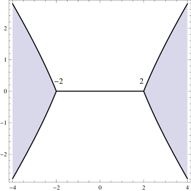
Figure 1: The set $\mathcal{X}_{0}$ and the regions $\mathop{\rm Re}\nolimits G(z)>0$ (shadowed regions) for the Gaussian model.

4 The cubic model

We will now discuss the cubic model

$$W(z)=\frac{z^{3}}{3}-tz,$$ (80)

where $t$ is an arbitrary complex number. For $t=0$ the model has been rigorously studied by Deaño, Huybrechs and Kuijlaars [29]. Recent results for $t\in\mathbb{R}$ have been communicated by Lejon [34]. The phase structure of the corresponding random matrix model has been studied by David [19] and Mariño [18].

4.1 The one-cut case

Using the notation specific for the one-cut case introduced in section 3.3 we have

$$y(z)=\left(z+\beta\right)\sqrt{(z-\beta)^{2}-\delta^{2}},\quad f(z)=-4z+b_{0},$$ (81)

and (50) and (51) lead to the following system of equations for the cut endpoints:

$$2\beta^{2}+\delta^{2}=2t,$$ (82)

$$\beta\delta^{2}=2.$$ (83)

Therefore $\beta$ satisfies the cubic equation

$$\beta^{3}-t\beta+1=0$$ (84)

and $\delta$ is determined by

$$\delta^{2}=\frac{2}{\beta}.$$ (85)

The cubic equation (84) defines a three-sheeted Riemann surface $\Xi$ of genus zero for $\beta$ as a function of $t$. The function $\beta(t)$ is determined in terms of three branches

$$\beta_{k}(t)=-\frac{t}{3\Delta_{k}}-\Delta_{k},\quad(k=0,1,2)$$ (86)

where

$$\Delta_{k}=\rme^{\rmi 2\pi k/3}\sqrt[3]{\frac{1}{2}+\sqrt{\frac{1}{4}-\left(\frac{t}{3}\right)^{3}}}$$ (87)

and where the roots take their respective principal values. There are three finite branch points

$$t^{(k)}=\frac{3}{2^{2/3}}\rme^{\rmi 2\pi k/3},\quad(k=0,1,2)$$ (88)

at which $\beta_{1}(t^{(0)})=\beta_{2}(t^{(0)})$, $\beta_{0}(t^{(1)})=\beta_{1}(t^{(1)})$, and $\beta_{0}(t^{(2)})=\beta_{2}(t^{(2)})$ respectively.

In the three separate plots of figure 2 we show the real parts of the three branches of the Riemann surface (84). As an aid to guide the eye, we also plot two paths on the surface. The first path starts at the origin $t=0$ in $\beta_{0}(t)$ (i.e., at $\beta_{0}(0)=-1$) and proceeds to the left without leaving this sheet. The second path corresponds to $|t|=3$ (larger than the modulus of the branch points $t^{(k)}$): note that the path stays in the branch $\beta_{0}(t)$ from the real axis $\arg t=0$ to $\arg t=2\pi/3$, proceeds to the $\beta_{1}(t)$ branch from $\arg t=2\pi/3$ to $\arg t=2\pi$, then to $\beta_{2}(t)$ from $\arg t=2\pi$ to $\arg t=10\pi/3$, and back to the branch $\beta_{0}(t)$ form $\arg t=10\pi/3$ to the real axis $\arg t=4\pi$.

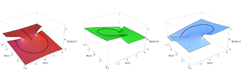
Figure 2: Real parts of the branches of $\beta(t)$.

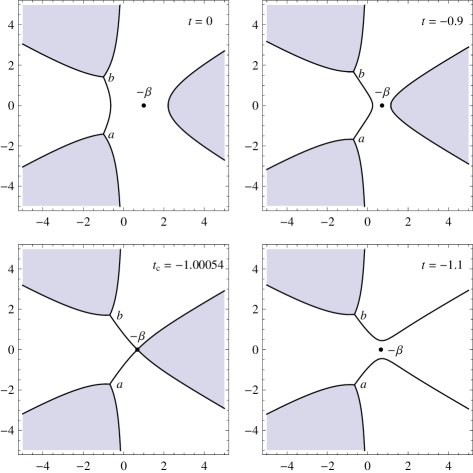
Figure 3: Sets $\mathcal{X}_{0}$ of Stokes lines calculated according to the branch $\beta_{0}(t)$ starting at $t=0$ and proceeding along the negative $t$ axis (path to the left in figure 2). The shaded areas are regions with $\mathop{\rm Re}\nolimits G(z)>0$.

Figure 3 shows the sets $\mathcal{X}_{0}$ of all the Stokes lines of the roots $a,b$ of the function $y^{2}(z)$ corresponding to $\beta_{0}(t)$ for negative real values of $t$. The path on $\beta_{0}(t)$ starts at $t=0$ and proceeds along the negative $t$ axis (the path to the left in figure 2). Note the two simple zeros $a$ and $b$, each one with three Stokes lines stemming at equal angles of $2\pi/3$. In the two first plots, corresponding to $t=0$ and $t=-0.9$, we find a short connecting $a$ and $b$, so that we get a cut satisfying the $S$-property. However, for a critical value $t_{\mathrm{c}}\approx-1.00054$ the double zero of $y^{2}(z)$ meets this cut giving rise to a singular curve, and beyond that point there is no Stokes line joining $a$ to $b$. This indicates that for $t<t_{\mathrm{c}}$ the branch $\beta_{0}(t)$ does not lead to a cut satisfying the $S$-property. (This interpretation is in agreement with the main theorem in [34].)

In fact, we can find an analytic condition (which, however, has to be solved numerically) for the set of complex values of $t$ such that $-\beta\in\mathcal{X}_{0}$, where $\mathcal{X}_{0}$ is the set of Stokes lines of $a$ and $b$. Using (68) we find that the $G$ functions corresponding to the branches $\beta_{k}(z)$ are

$$G_{k}(z) = \frac{1}{3}\sqrt{(z-\beta_{k})^{2}-\delta_{k}^{2}}\left(z^{2}+\beta_{k}z+\beta_{k}^{2}-3t+\frac{\delta_{k}^{2}}{2}\right)$$ (89)

$${}-\log\left(\frac{\beta_{k}-z-\sqrt{(z-\beta_{k})^{2}-\delta_{k}^{2}}}{\delta_{k}}\right)^{2}.$$

Hence the condition for $-\beta_{k}\in\mathcal{X}_{0}$ is

$$\mathop{\rm Re}\nolimits G_{k}(-\beta_{k}(t))=0,$$ (90)

where

$$G_{k}(-\beta_{k})=-\frac{1}{3}\sqrt{4\beta_{k}^{2}-\delta_{k}^{2}}\left(2\beta_{k}^{2}+\delta_{k}^{2}\right)-\log\left(\frac{2\beta_{k}-\sqrt{4\beta_{k}^{2}-\delta_{k}^{2}}}{\delta_{k}}\right)^{2}.$$ (91)

In figure 4 we show the curves in the complex $t$-plane determined by the solutions of (90), with colors matching those of the corresponding branches in figure 2. In addition each region has been identified with a number that will be used in our forthcoming discussion of the phase structure.

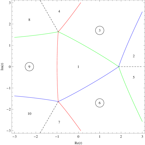
Figure 4: The solid lines represent the solutions of (90) for $k=0,1,2$, with colors matching those of the respective branches in figure 2. The dashed lines are the cuts ($|t|>3/2^{2/3},\;\arg t=0,\pm 2\pi/3$) of the Riemann surface (84).

4.2 The two-cut case

In the two-cut case we will denote $a_{1}^{-}=a$, $a_{1}^{+}=b$, $a_{2}^{-}=c$, $a_{2}^{+}=d$ and $r_{1}=r$. Now we have

$$y(z)=\sqrt{(z-a)(z-b)(z-c)(z-d)},\quad f(z)=-4z+b_{0},$$ (92)

and (50), (51) and (52) lead the following system of equations for the four cut endpoints

$$abc+abd+acd+bcd=4,$$ (93)

$$ab+ac+bc+ad+bd+cd=-2t,$$ (94)

$$a+b+c+d=0,$$ (95)

$$\int_{b}^{c}y(z_{+})\rmd z=\rmi r.$$ (96)

We recall that $r$ is given in terms of $B$-periods

$$B(\rmd\omega)=\oint_{B}\rmd\omega=-2\int_{a}^{b}\rmd\omega$$ (97)

(we drop the subindex, i.e., $B=B_{1}$) by equation (48)

$$r=\frac{\mathop{\rm Re}\nolimits B\left(\frac{1}{3}\rmd\Omega_{3}-t\rmd\Omega_{1}-\rmd\Omega_{0}\right)}{\mathop{\rm Im}\nolimits B(\rmd\varphi)}.$$ (98)

Taking into account that (93)–(95) imply

$$y(z)=z^{2}-t-\frac{2}{z}+\cdots,\quad z\rightarrow\infty,$$ (99)

it follows that

$$r=\frac{\mathop{\rm Re}\nolimits\left(\mathcal{B}_{4}-2t\mathcal{B}_{2}-4\mathcal{B}_{1}+C\mathcal{B}_{0}\right)}{\mathop{\rm Im}\nolimits\left(\mathcal{B}_{0}/\mathcal{A}_{0}\right)},$$ (100)

where $\mathcal{A}_{n}$, $\mathcal{B}_{n}$ denote the integrals

$$\mathcal{A}_{n}=\int_{b}^{c}\frac{z^{n}}{y(z_{+})}\rmd z,\quad\mathcal{B}_{n}=\int_{a}^{b}\frac{z^{n}}{y(z_{+})}\rmd z,$$ (101)

and

$$C=\frac{-\mathcal{A}_{4}+2t\mathcal{A}_{2}+4\mathcal{A}_{1}}{\mathcal{A}_{0}}.$$ (102)

It is clear that in general the system (93)–(96) must be solved numerically. But even so, it would be very difficult to attempt a direct numerical solution without a well identified initial approximation. However, we can take advantage of our knowledge of the critical curves (90) and the corresponding explicit solutions for the one-cut endpoints given by (86), and proceed iteratively by small increments in $t$ using as initial approximation at each step the results of the previous one. Once the cut endpoints $a$, $b$, $c$ and $d$ for a certain value of $t$ have been calculated, the corresponding Stokes lines are also calculated numerically.

Figures 5 and 6 show the sets $\mathcal{X}_{0}=\mathcal{X}$ of all the Stokes lines stemming from the simple roots $a$, $b$, $c$ and $d$ for values of $t$ crossing critical lines of figure 4. In figure 5 we proceed along the negative $t$ axis beyond the critical value $t_{\mathrm{c}}\approx-1.00054$ (i.e., to the part of the path corresponding to $t<-1.00054$ in the first graph of figure 2) and we find a “splitting of a cut” at the crossing from region 1 to region 9 in figure 4, in agreement with the theoretical result of [34]. In figure 6 we have crossed vertically from region 8 into region 9, and find a process of “birth of a cut at a distance” with cut endpoints $c$ and $d$; the graph corresponding to $t=-1.5$, not shown in the figure, is precisely the last graph in figure 5; and as we proceed further down from region 9 to region 10 we find the symmetric “death of a cut at a distance” with cut endpoints $a$ and $b$. In the next section these interpretations are confirmed by numerical calculations of zeros of orthogonal polynomials.

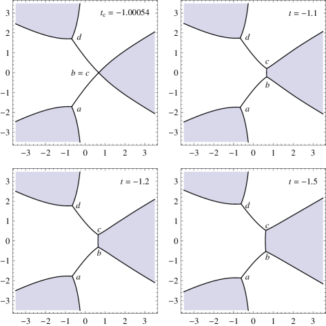
Figure 5: Splitting of a cut.

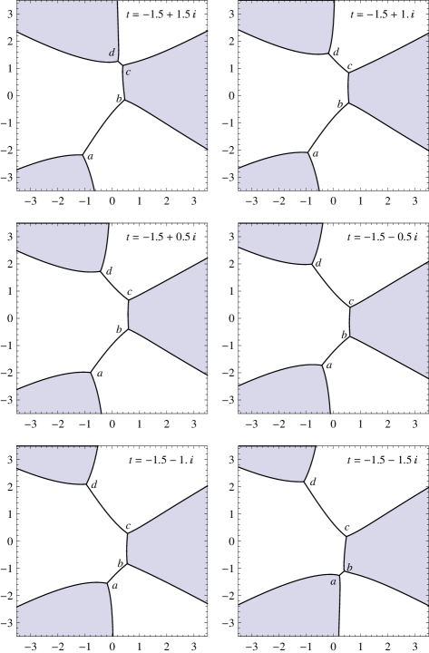
Figure 6: Birth and death of a cut at a distance .

4.3 Asymptotic zero distributions of orthogonal polynomials

As we discussed in section 2.1, to determine the asymptotic zero distribution of a given family of orthogonal polynomials (1) on a path $\Gamma$, we must find an $S$-curve in the same homology class as $\Gamma$ and connecting the same pair of convergence sectors at infinity. Then the desired zero counting measure is the equilibrium measure on the $S$-curve.

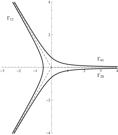
Figure 7: Infinite simple curves connecting convergence sectors of the complex cubic model.

The cubic exponential weight $\exp(-n(z^{3}/3-tz))$ decays in three sectors $S_{k}$ of opening $\pi/3$ of the complex $z$ plane centered around the rays $\lambda_{k}=\{z:\arg z=2\pi k/3\}$, $k=0,1,2$. Let us denote by $\Gamma_{ij}$ $(i\neq j)$ simple paths with asymptotic directions $\lambda_{i}$ and $\lambda_{j}$ as indicated in figure 7 and, for concreteness, consider the problem of determining $S$-curves $\Gamma$ in the same homology class and with the same asymptotic directions of $\Gamma_{12}$. The graph corresponding to $t=0$ in figure 3 shows that the cut $ab$ can be prolonged both upwards and downwards into the shaded regions which contain the asymptotic directions $\lambda_{1}$ and $\lambda_{2}$ respectively, and therefore into a full $S$-curve homologous to $\Gamma_{12}$. This is no longer true for $t<t_{\mathrm{c}}$, as the graph corresponding to $t=-1.1$ in figure 3 shows: in fact, the cut $ab$ has disappeared. However, the graph for $t=-1.1$ in figure 5 features the two cuts $ab$ and $cd$, which can be prolonged into the same sectors via the shaded region in the right part of the figure. Therefore, for this value of $t$ we have a full two-cut $S$-curve.

This type of analysis which combines the theoretical results of section 3 with numerical calculations show that in the case of $\Gamma_{12}$ the branches $\beta_{0}$, $\beta_{1}$ and $\beta_{2}$ can be used to generate a one-cut $S$-curve for the cubic model when $t$ is in the regions 1 to 7, 8 and 10 of figure 4, respectively. For $\Gamma_{12}$ the encircled region 9 represents the two-cut region. Similar (symmetric) situations arise for the cases of $\Gamma_{01}$ and $\Gamma_{20}$, for which the two-cut regions are the encircled regions 3 and 6 respectively.

As a check of the consistency of these results with Theorem 1, in figures 8, 9 and 10 we superimpose to the graphs of figures 3, 5 and 6 the zeros of the corresponding polynomials $p_{n}(z)$ with degree $n=24$, which we have generated by recurrence formulas to minimize numerical errors. In figures 8 and 9, which exemplify the splitting of a cut, as $t$ decreases along the negative real axis and due to the symmetry of the situation, the 24 zeros split evenly into the two sets of 12 zeros following closely the positions of the cuts that correspond to the limit $n\to\infty$. In figure 10, which exemplifies the birth and death of a cut at a distance, what we find numerically as the value of $t$ descends vertically from $t=-1.5+1.5\rmi$ to $t=-1.5-1.5\rmi$ is that all the 24 zeros lie initially on the lower cut $ab$, and start travelling upwards one by one, thus populating the upper cut $cd$ and depopulating the lower $ab$. This behavior is particularly clear in the second graph (corresponding to $t=-1.5+\rmi$), in which the fourth zero is “arriving” at the upper cut, and in the symmetric graph (corresponding to $t=-1.5-\rmi$), in which the 21st zero is “leaving” the lower cut.

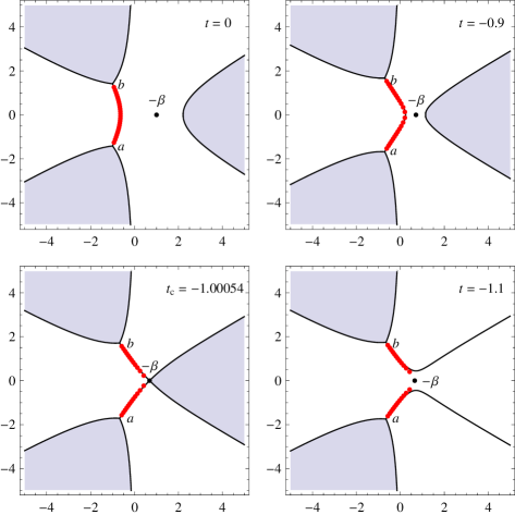
Figure 8: Zeros of $p_{24}(z)$ superimposed to the splitting of a cut in figure 3.

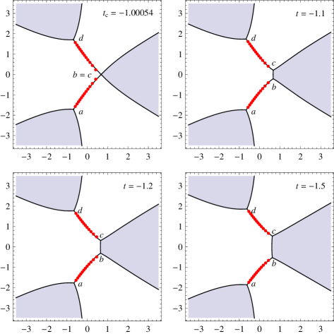
Figure 9: Zeros of $p_{24}(z)$ superimposed to the splitting of a cut in figure 5.

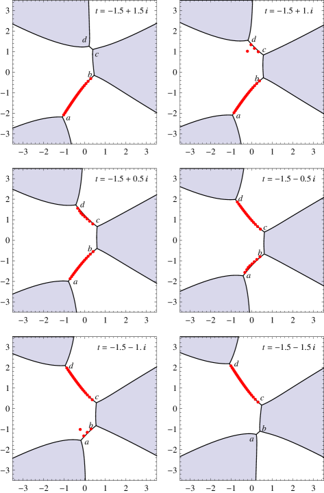
Figure 10: Zeros of $p_{24}(z)$ superimposed to the birth and death of a cut at a distance in figure 6.

A phase diagram for the cubic random matrix model with a two-cut region with the same shape as region 3 in figure 4 was presented in [19]. It is also worth noticing that in terms of the variable $w=t^{-3/2}$ the curve (90) looks quite similar to the genus 0 breaking curve found in [35] for the family of orthogonal polynomials associated to the quartic potential

$$W(z)=\frac{w}{4}z^{4}+\frac{1}{2}z^{2}.$$ (103)

However, the curve in [35] is only symmetric with respect the real $w$-axis, while the curve for the cubic model is symmetric with respect both real and imaginary axes. Another important difference between the curve for the cubic model and that for the quartic model is that for this later there exist genus 0 and genus 1 breaking curves (see figure 4 in [35]), although implicit equations for genus 1 curves are provided only for the symmetric case [35].

5 Generalizations and concluding remarks

A generalization of the $S$-property (19) arises in the study of dualities between supersymmetric gauge theories and string models on local Calabi-Yau manifolds $\mathcal{M}$ of the form [14, 15, 16, 36, 37, 38, 39]

$$W^{\prime}(z)^{2}+f(z)+u^{2}+v^{2}+w^{2}=0,$$ (104)

where $W(z)$ and $f(z)$ are polynomials such that $\deg f=\deg W-2$. The manifold $\mathcal{M}$ can be regarded as a fibration of two-dimensional complex spheres on the spectral curve $y^{2}=W^{\prime}(z)^{2}+f(z)$. Most of the string model information encoded in $\mathcal{M}$ can be described in terms of the spectral curve, and its associated complex density (31). These spectral curves satisfy the condition (19) for the $S$-property, but they do not determine an equilibrium density since (31) provides in general a complex density. As a consequence the complex electrostatic potential is locally constant on the support of $\rho(z)$

$$\mathcal{U}(z)=L_{j},\quad z\in\gamma_{j},\quad j=1,\ldots,s,$$ (105)

but the real parts of the constants $L_{j}$ are, in general, different. In this case the cut endpoints are determined by (50), (51) and, instead of (52), by the constraints

$$\int_{\gamma_{j}}\rho(z)|\rmd z|=S_{j},$$ (106)

where $\rho(z)$ is the complex density (31) and $S_{j}$ are a given set of nonzero complex values (’t Hooft parameters). Finally, instead of the single quadratic differential $y^{2}(z)(\rmd z)^{2}$, in this case $s$ in general different quadratic differentials $\rme^{-\rmi 2\arg S_{j}}y^{2}(z)(\rmd z)^{2}$ are required to determine the cuts $\gamma_{j}$ as Stokes lines

$$\mathop{\rm Re}\nolimits\left(\rme^{-\rmi\arg S_{j}}\int_{a_{j}^{-}}^{z}y(z)\rmd z\right)=0,\quad z\in\gamma_{j}.$$ (107)

We believe that these more general spectral curves can be characterized and classified using an analysis similar to that of the present paper.

Appendix A

In this appendix we briefly discuss the elements of the theory of Abelian differentials in Riemann surfaces that we use in section 3.1.

Let us denote by $M$ the hyperelliptic Riemann surface associated to the curve (39). The two branches $w_{1}(z)$ and $w_{1}(z)=-w_{2}(z)=w(z)$ characterize $M$ as a double-sheeted covering of the extended complex plane:

$$M=M_{1}\cup M_{2},\quad M_{i}=\{Q=(w_{i}(z),z)\}.$$ (108)

The homology basis $\{A_{i},B_{i}\}_{i=1}^{s-1}$ of cycles in $M$ is defined as shown in figure 11, and the corresponding periods of a differential $\rmd\omega$ in $M$ will be denoted by

$$A_{i}(\rmd\omega)=\oint_{A_{i}}\rmd\omega,\quad B_{i}(\rmd\omega)=\oint_{B_{i}}\rmd\omega.$$ (109)

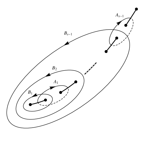
Figure 11: Homology basis.

We introduce the following Abelian differentials in $M$:

(1)

The canonical basis of first kind (i.e., holomorphic) Abelian differentials $\{\rmd\varphi_{i}\}_{i=1}^{s-1}$ with the normalization $A_{i}(\rmd\varphi_{j})=\delta_{ij}$. These differentials can be written as

$$\rmd\varphi_{j}(z)=\frac{p_{j}(z)}{w(z)}\rmd z,$$ (110)

where the $p_{j}(z)$ are polynomials of degree not greater than $s-2$ uniquely determined by the normalization conditions.

(2)

The second kind Abelian differentials $\rmd\Omega_{k}$ $(k\geq 1)$ whose only poles are at $\infty_{1}$, such that

$$\rmd\Omega_{k}(Q)=(kz^{k-1}+\mathcal{O}(z^{-2}))\rmd z,\quad Q\rightarrow\infty_{1},\quad z=z(Q),$$ (111)

and normalization $A_{i}(\rmd\Omega_{k})=0$ $(i=1,\ldots,s-1)$. It is easy to see that

$$\rmd\Omega_{k}=\left(\frac{k}{2}z^{k-1}+\frac{P_{k}(z)}{w(z)}\right)\rmd z,$$ (112)

where the $P_{k}(z)$ are polynomials of the form

$$P_{k}(z)=\frac{k}{2}(z^{k-1}w(z))_{\oplus}+\sum_{i=0}^{s-2}c_{ki}z^{i}$$ (113)

and the coefficients $c_{ki}$ are uniquely determined by the normalization conditions.

(3)

The third kind Abelian differential $\rmd\Omega_{0}$ whose only poles are at $\infty_{1}$ and $\infty_{2}$, such that

$$\rmd\Omega_{0}(Q)=\left\{\begin{array}[]{ll}\displaystyle\left(\frac{1}{z}+\mathcal{O}(z^{-2})\right)\rmd z,&Q\rightarrow\infty_{1}\\ \displaystyle\left(-\frac{1}{z}+\mathcal{O}(z^{-2})\right)\rmd z,&Q\rightarrow\infty_{2},\end{array}\right.\quad z=z(Q).$$ (114)

and normalization $A_{i}(\rmd\Omega_{0})=0$ for all $i=1,\ldots,s-1$. It follows that

$$\rmd\Omega_{0}=\frac{P_{0}(z)}{w(z)}\rmd z,$$ (115)

where $P_{0}(z)$ is a polynomial of the form

$$P_{0}(z)=(z^{-1}w(z))_{\oplus}+\sum_{i=0}^{s-2}c_{0i}z^{i}$$ (116)

and the coefficients $c_{0i}$ are uniquely determined by the normalization conditions.

For instance, in the one-cut case ($s=1$) we have

$$P_{k}(z)=\left(\delta_{k0}+\frac{k}{2}\right)\left(z^{k-1}\sqrt{(z-a)(z-b)}\right)_{\oplus},$$ (117)

and the first three polynomials are

$$P_{0}(z)=1,$$ (118)

$$P_{1}(z)=\frac{1}{2}z-\frac{1}{4}(a+b),$$ (119)

$$P_{2}(z)=z^{2}-\frac{1}{2}(a+b)z-\frac{1}{8}(a-b)^{2}.$$ (120)

References

References

- [1] Stahl H 1985 Complex Variables Theory Appl. 4 311
- [2] Stahl H 1985 Complex Variables Theory Appl. 4 325
- [3] Stahl H 1986 Constructive Approximation 2 225
- [4] Stahl H 1986 Constructive Approximation 2 241
- [5] Gonchar A A and Rakhmanov E A 1989 Math. USSR Sbornik 62 305
- [6] Rakhmanov E A 2012 Contemp. Math. 578 195
- [7] Martínez-Finkelshtein A and Rakhmanov E A 2011 Commun. Math. Phys. 302 53
- [8] Deift P, Kriecherbauer T, McLaughlin K T R, Venakides S and Zhou X 1999 Commun. Pure. Appl. Math. 52 1335
- [9] Bleher P and Its A 1999 Ann. Math. 150 185
- [10] Bleher P and Its A 2003 Commun. Pure Appl. Math. 56 433
- [11] Bleher P 2008 Lectures on random matrix models. The Riemann-Hilbert approach (Amsterdam: North Holland)
- [12] Bertola M and Mo M Y 2009 Adv. Math. 220 154
- [13] Bertola M 2011 Analysis and Math. Phys. 1 167
- [14] Cachazo F, Intriligator K and Vafa C 2001 Nuc. Phys. B 603 3
- [15] Dijkgraaf R and Vafa C 2002 Nuc. Phys. B 644 3
- [16] Dijkgraaf R and Vafa C 2002 Nuc. Phys. B 644 21
- [17] Heckman J J, Seo J and Vafa C 2007 J. High Energy Phys. 07 073
- [18] Mariño M, Pasquetti S and Putrov P 2010 J. High Energy Phys. 10 074
- [19] David F 1991 Nuc. Phys. B 348 507
- [20] David F 1993 Phys. Lett. B 302 403
- [21] Deift P 1999 Orthogonal Polynomials and Random Matrices: A Riemann-Hilbert approach (Providence: American Mathematical Society)
- [22] Felder G and Riser R 2004 Nuc. Phys. B 691 251
- [23] Lazaroiu C I 2003 J. High Energy Phys. 03 044
- [24] Saff E and Totik V 1997 Logarithmic Potentials with External Fields (Berlin: Springer)
- [25] Álvarez G, Martínez Alonso L and Medina E 2010 J. Stat. Mech. Theory Exp. 03023
- [26] Gonchar A A and Rakhmanov E A 1984 Math. USSR Sbornik 125 117
- [27] Nadal C and Majumdar S N 2011 J. Stat. Mech. Theory Exp. 04001
- [28] Álvarez G, Martínez Alonso L and Medina E 2011 Nuc. Phys. B 848 398
- [29] Deaño A, Huybrechs D and Kuijlaars A B J 2010 J. Approx. Theory 162 2202
- [30] Itoyama H and Morozov A 2003 Nuc. Phys. B 657 53
- [31] Itoyama H and Morozov A 2003 Prog. Theor. Phys. 109 433
- [32] Farkas H M and Kra I 1991 Riemann Surfaces (Springer)
- [33] Sibuya Y 1975 Global Theory of a Second Order Linear Ordinary Differential Equation with a Polynomial Coefficient (North-Holland)
- [34] Lejon N 2012 Zero distribution of complex orthogonal polynomials with respect to some exponential weights Tech. Rep. Department of Mathematics, KU Leuven, Netherlands
- [35] Bertola M and Tovbis A Asymptotics of orthogonal polynomials with complex varying quartic weight: global structure, critical point behavior and the first Painlevé equation arXiv1108.0321
- [36] Di Francesco P, Ginsparg P and Zinn-Justin J 1995 Phys. Rep. 254 1
- [37] Seiberg N and Witten E 1994 Nuc. Phys. B 426 19
- [38] Becker K, Becker E and Strominger A 1995 Nuc. Phys. B 456 130
- [39] Cachazo F, Seiberg N and Witten E 2003 J. High Energy Phys. 03 042