Interaction and disorder effects in 3D topological insulator thin films

Abstract

A theory of combined interference and interaction effects on the diffusive transport properties of 3D topological insulator surface states is developed. We focus on a slab geometry (characteristic for most experiments) and show that interactions between the top and bottom surfaces are important at not too high temperatures. We treat the general case of different surfaces (different carrier densities, uncorrelated disorder, arbitrary dielectric environment, etc.). In order to access the low-energy behavior of the system we renormalize the interacting diffusive sigma model in the one loop approximation. It is shown that intersurface interaction is relevant in the renormalization group (RG) sense and the case of decoupled surfaces is therefore unstable. An analysis of the emerging RG flow yields a rather rich behavior. We discuss realistic experimental scenarios and predict a characteristic non-monotonic temperature dependence of the conductivity. In the infrared (low-temperature) limit, the systems flows into a metallic fixed point. At this point, even initially different surfaces have the same transport properties. Investigating topological effects, we present a local expression of the $\mathbb{Z}_{2}$ theta term in the sigma model by first deriving the Wess-Zumino-Witten theory for class DIII by means of non-abelian bosonization and then breaking the symmetry down to AII. This allows us to study a response of the system to an external electromagnetic field. Further, we discuss the difference between the system of Dirac fermions on the top and bottom surfaces of a topological insulator slab and its non-topological counterpart in a double-well structure with strong spin-orbit interaction.

I Introduction

Topological states of matter have recently attracted immense scientific interest which was in particular boosted by the theoretical predictionBernevig and Zhang (2006); Bernevig et al. (2006); Fu et al. (2007); Moore and Balents (2007); Roy (2009) and subsequent experimental discoveryKönig et al. (2007); Hsieh et al. (2008) of two-dimensional (2D) and three-dimensional (3D) time reversal invariant topological insulators.

In their bulk, topological insulatorsHasan and Kane (2010); Qi and Zhang (2011); Schnyder et al. (2008); Kitaev (2009) (TI) are electronic band insulators characterized by a topological invariant which accounts for the non-trivial structure of the Bloch states. In contrast, the interface between two topologically different phases (e.g. TI - vacuum) hosts gapless, extended boundary states. Their appearance is topologically protected via the bulk-boundary correspondence.Gurarie (2011) In retrospect we understand that the quantum Hall effect (QHE)Klitzing et al. (1980) at given quantized transverse conductance was the first example of a topological insulator: The Landau levels provide the bulk band gap which is accompanied by the topological TKNNThouless et al. (1982) number and the protected chiral edge states.

In contrast to the QHE, the newly discovered 2D and 3D topological insulators require the absence of magnetic field and rely on strong spin-orbit interaction. Further, their topological invariant takes only values in $\mathbb{Z}_{2}$ (contrary to the TKNN integer). The 2D TI phase (also known as quantum spin Hall state) was experimentally identified by the characteristic quantized value $2e^{2}/h$ of the two-point conductance in HgTe quantum wells.König et al. (2007) The discriminating feature of all 3D TI is the massless Dirac states on the 2D boundary which were first spectroscopically detected in BiSbHsieh et al. (2008) alloys and subsequently in many other materials.Hasan and Kane (2010) To present date, various experimental groups confirmed predominant surface state transport (for a review see Ref. Culcer, 2012), in particular elucidating ambipolar field-effectSteinberg ; CheckelskyHor2011 ; KimFuhrer2012 ; HongCui2012 ; KimQuiziFuhrer2012 and the typical QHE-steps of Dirac electrons,ChengChen2010 ; HanaguriSasagawa2010 ; AnalytisFisher2010 ; SacepeMorpurgo2011 ; Brüne et al. (2011) Aharonov-Bohm oscillationsPengCui2010 ; XiuWang2011 ; DufouleurGiraud2013 as well as weak antilocalization (WAL) corrections in the magnetoconductivity data.SteinbergPRB ; ZhangLi2011 ; Chen et al. (2011) Moreover, several transport experiments reveal the importance of electron-electron interactions in 3D TI materials.Chen et al. (2011); Wang ; Liu

Inspired by recent experimental advances, we present here a detailed analysis of interference and interaction corrections to conductivity in the most conventional setup for transport experiments: the slab geometry, in which the 3D TI films are rather thin (down to $\sim 10$ nm) although still thick enough to support well separated surface states. As we will explain in more detail, the long-range Coulomb interaction between the two major surfaces plays an important role. We derive the quantum corrections to conductivity in the diffusive regime by taking into consideration the WAL effect as well as corrections of Altshuler-Aronov type Alt (1985) induced by inter- and intrasurface interaction. We consider the general situation of different surfaces subjected to different random potentials, mismatch in carrier densities and unequal dielectric environment.

The present paper constitutes a natural extension of the previous workOstrovsky et al. (2010) by three of the authors in which a single 3D TI surface was analyzed. It was found that the interplay of topological protection and interaction- and interference-induced conductivity corrections drives the system into a novel critical state with longitudinal conductance of the order of $e^{2}/h$. As we show below, the intersurface interaction in a thin TI slab makes the overall picture much more complex and crucially affects the ultimate infrared behavior.

In another recent paper, Burmistrov et al. (2011) two of us were involved in the theoretical investigation of inter- and intrawell interaction effects in double quantum well heterostructures studied experimentally in Ref. Minkov et al., 2011. Let us point out key differences between the present paper and that work. First, in Ref. Burmistrov et al., 2011 only equal carrier densities were considered. Second, disorder was assumed to be the same in both quantum wells (and thus completely correlated). This affects the soft-mode content of the low-energy theory. Third, quantum wells host electrons with spin degeneracy which can be lifted by a magnetic field. As a consequence, i) electrons in double quantum well fall into a symmetry class different from that of 3D TI and ii) more interaction channels have to be included. These subtleties affect in a crucial way the renormalization group (RG) flow: according to the analysis of Ref. Burmistrov et al., 2011, the interwell interaction becomes irrelevant at low energies, which is opposite to what we find in the two-surface TI model in the present paper. Finally, the TI problem shows topology-related effects that were absent in the double quantum well structure.

As in the two preceding works, we here use the interacting, diffusive non-linear sigma model (NL$\sigma$M) approach to capture the diffusive low-energy physics. Quantum corrections to the longitudinal conductivity $\sigma$ are obtained by renormalization of this effective action in the one loop approximation (i.e. perturbatively in $1/\sigma$ but exactly in interaction amplitudes). The interacting NL$\sigma$M was originally developed by Finkel’stein in the eighties A.M.Finkel’stein (1983, 1984) (for review articles see Ref.s Finkelstein, 1990; Belitz and Kirkpatrick, 1994; Finkel’stein, 2010). In addition to perturbative RG treatment (which can also be performed diagrammatically Castellani et al. (1984)) it also allows one to incorporate topological effects and was thus a fundamental tool for understanding the interplay of disorder and interactions in a variety of physical problems, including the superconducting transition in dirty films, Finkel’stein (1987, 1994) the integer QHE, A.M.M. Pruisken (1995); Pruisken and Burmistrov (2007) and the metal-insulator transition in Si MOSFETs. Punnoose and Finkel’stein (2005)

Analyzing the RG equations for the thin 3D TI film, we find that (in contrast to the previous work on the double quantum well structure) the intersurface interaction is relevant in the RG sense. The system flows towards a metallic fixed point at which even two originally different surfaces are characterized by the same conductivities. As we discuss in detail below, the hallmark of the intersurface interaction in 3D TI transport experiments is a characteristic non-monotonic temperature dependence of the conductivity. In contrast to the case of decoupled surfaces, due to the intersurface interaction, quantum corrections to the conductivity depend on the carrier densities.

The paper is structured as follows. In Sec. II we expose in detail the theoretical implications of a typical experimental slab geometry setup, demonstrate the relevance of intersurface interaction and introduce the microscopic fermionic Hamiltonian. Subsequently (Sec. III), we use the non-Abelian bosonization technique to map the fermionic theory on the ($\mathbf{U}\left(1\right)$-) gauged, interacting NL$\sigma$M with $\mathbb{Z}_{2}$ topological term. Here we also discuss the Fermi liquid treatment of generally strong electron-electron interactions. Next, we renormalize the NL$\sigma$M in Sec. IV. Sections III and IV contain both pedagogical explanations and important details for experts. Readers purely interested in the results can jump to Sec. V, where the RG flow and the implied phase diagram are analyzed. Detailed predictions for typical experiments can be found in Sec. VI. We close the paper by summarizing our results and discussing prospects for future work in Sec. VII.

II Topological insulator slabs: Experimental setup and theoretical model

II.1 Setup

In this work we analyze the effect of interaction on transport properties of strong 3D topological insulator thin films in the diffusive regime. While we mainly focus on the theoretically most interesting case of purely surface transport, we also show that our theory can easily be extended to a case when only a part of the sample is in the topological phase, i.e. one has a conduction through a topologically protected surface spatially separated from a thick (bulk) conducting region.

A typical experimental setup is shown in Fig. 1. Our analysis is valid in the regime where the penetration depth of surface states $a$ is small with respect to the film thickness $d$. We therefore neglect intersurface tunneling (which would destroy the topological protection). Further, we assume the disorder correlation length (depicted by the range of the impurity potentials) to be small $\xi\ll d$. We treat a generic case when the vicinity to the coat or, respectively, to the substrate may induce a different degree of disorder on the top and bottom surfaces. We thus consider the corresponding mean free paths $l_{1}$ and $l_{2}$ as two independent parameters. Moreover, we also allow the chemical potentials $\mu_{1}$ and $\mu_{2}$ on the two surfaces to be different. (By convention we set $\mu_{s}=0$ at the Dirac point. Here and below $s=1,2$ denotes the surface index.) The chemical potentials may be experimentally controlled by means of electrostatic gates. As has been stated above, we mostly focus on the situation where both $\mu_{1}$ and $\mu_{2}$ lie well within the bulk gap $\Delta_{\rm bulk}$. The extension of our results to the experimentally important regime when only one of chemical potentials is located within the bulk gap, $|\mu_{1}|\ll\Delta_{\rm bulk}\lesssim|\mu_{2}|$, can be found in section V.2.1.

If the electrostatic gates are present and too close to the sample, Coulomb interaction is externally screened and the electron-electron interaction is purely short range. However, such an experimental scenario is a rare exception from the rule. Therefore, in the main text we assume sufficiently distant gates and concentrate on the limit of long-range Coulomb interaction. In addition we derive general RG equations (Appendix D) which allow us to explore the crossover from the long-range case to the short-range one, see Appendix F. Qualitatively, the RG flow for a sufficiently strong short-range interaction in the case of externally screened surfaces turns out to be similar to the flow in the absence of external screening.

Since we assume that the thickness $d$ of the sample is much smaller than its other linear dimensions, we neglect contributions of four side faces of the slab (whose area is proportional to $d$).

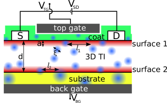
Figure 1: Scheme of a typical experimental setup. The hierarchy of length scales is explained in the main text.

The goal of the present analysis is to study conduction properties of thin 3D TI films in the diffusive regime, i.e., at energy scales $E$ far below the elastic scattering rates $1/\tau_{s}$ of both surfaces,

$$E\ll\min_{s=1,2}\hbar/{\tau_{s}}\,.$$ (1)

In turn the elastic scattering rates are assumed to be small compared to the chemical potentials

$$\hbar/\tau_{s}\ll|\mu_{s}|.$$ (2)

In experiment $E$ is set by the AC frequency ($E=\hbar\omega$) or by temperature ($E=k_{B}T$), whichever of the two is larger. Equation (1) is equivalent to the hierarchy of length scales

$$l\ll L_{E}\,,$$ (3)

where we have introduced the maximal mean free path $l=\max_{s=1,2}l_{s}$ and the length scale $L_{E}=\min_{s=1,2}(\hbar D_{s}/E)^{1/2}$, with $D_{s}$ being the diffusion coefficients for the two surfaces.

II.2 Interaction

Can Coulomb interaction between the top and bottom surface states play an important role in the experiment? To answer this question, we compare the sample thickness with all natural length scales of the system: the screening length $l_{\rm scr}$, the (maximal) mean free path $l$ and the experimentally tunable scale $L_{E}$.

The Coulomb interaction is (throughout the paper underlined symbols denote $2\times 2$ matrices in the surface space)

$$\underline{U}_{0}\left(\textbf{{r}}\right)=\frac{e^{2}}{\epsilon}\left(\begin{array}[]{cc}\frac{1}{r}&\frac{1}{\sqrt{r^{2}+d^{2}}}\\ \frac{1}{\sqrt{r^{2}+d^{2}}}&\frac{1}{r}\end{array}\right).$$ (4)

The two dimensional vector r connects the two dimensional positions of the particles, $r=|{\bf r}|$, $e$ is the charge of the electrons, and $\epsilon$ denotes the effective dielectric constant.

Fourier transformation and RPA-screening leads to Zheng and MacDonald (1993); Kamenev and Oreg (1995); Flensberg et al. (1995); Burmistrov et al. (2011) ($U\equiv U\left(\textbf{{q}}\right)\equiv 2\pi e^{2}/\epsilon q$)

$$\underline{U}_{\rm scr}\left(\textbf{{q}}\right)=\frac{\underline{U}}{1-\left(\Pi_{1}+\Pi_{2}\right)U+U^{2}\Pi_{1}\Pi_{2}\left(1-e^{-2dq}\right)}$$ (5)

with

$$\underline{U}=U\left(\begin{array}[]{cc}1-\Pi_{2}U\left(1-e^{-2dq}\right)&e^{-dq}\\ e^{-dq}&1-\Pi_{1}U\left(1-e^{-2dq}\right)\end{array}\right).$$

Here $\Pi_{s}$ is the polarization operator of the surface states.

In the present section we will concentrate on the statically screened interaction potential. In this limit the polarization operator is determined by the thermodynamic density of states: $\Pi_{s}\left(\omega=0,\textbf{{q}}\right)=-\nu_{s}$.

In the diffusive regime defined by the condition (3), the wavevector $q$ satisfies the inequality $1/L_{E}\ll q\ll 1/l$. Therefore, in a sample of thickness $d\gg L_{E}$ we always have $dq\gg 1$ and the two surfaces decouple,

$$\underline{U}_{\rm scr}\stackrel{{\scriptstyle d\gg L_{E}}}{{=}}2\pi\frac{e^{2}}{\epsilon}\left(\begin{array}[]{cc}\frac{1}{q+\kappa_{1}}&0\\ 0&\frac{1}{q+\kappa_{2}}\end{array}\right),$$ (6)

where $\kappa_{s}=2\pi e^{2}\nu_{s}/\epsilon$ is the inverse Thomas-Fermi screening length for a single surface $s$. A universal form of the Altshuler-Aronov correction to conductivity induced by the Coulomb interaction Alt (1985); Ostrovsky et al. (2010) arises in the unitary limit when one can neglect $q$ as compared with $\kappa_{s}$ in Eq.(6). The unitary limit is achieved if $\kappa_{s}^{-1}\ll l$ (the meaning of this condition as well as the complementary case are discussed in section III.6.3).

In the opposite limit of a small interlayer distance, $d\ll l$, we can approximate $e^{-dq}\approx 1$ in the whole diffusive regime. This implies

$$\underline{U}_{\rm scr}\stackrel{{\scriptstyle d\ll l}}{{=}} \displaystyle\frac{2\pi e^{2}}{\epsilon}\frac{1}{q+\kappa_{1}+\kappa_{2}+2d\kappa_{1}\kappa_{2}\left(1-qd\right)}$$ (9)

$$\times\left(\begin{array}[]{cc}1+2\kappa_{2}d&1\\ 1&1+2\kappa_{1}d\end{array}\right).$$

At the first glance, it looks as if also negative interaction potential was possible. However, this is not the case as shall be explained in what follows. Depending on the hierarchy of the lengthscales $\kappa_{1}^{-1},\kappa_{2}^{-1}$ and $d$ the following scenarios are conceivable:

First, consider $\kappa_{s}d\ll 1$ for both $s=1$ and $s=2$. In this case, the $q$ dependence of the interaction potential implies the definition of the coupled layer screening length $l_{\rm scr}$:

$$\left(\underline{U}_{\rm scr}\right)_{ss^{\prime}}\left(\textbf{{q}}\right)\sim\frac{1}{q+\kappa_{1}+\kappa_{2}}\ \ \Rightarrow\ \ l_{\rm scr}=\frac{1}{\kappa_{1}+\kappa_{2}}.$$ (10)

If in addition the condition $l_{\rm scr}\ll l$ is fulfilled, the Coulomb interaction potential (9) becomes “overscreened” ($q$-independent) for all diffusive momenta $q\ll l^{-1}$.

Second, assume that $\kappa_{s}d\gg 1$ for at least one surface. Then the $q$-dependence of $\underline{U}_{\rm scr}$ is always negligible and thus the notion of coupled layer screening length is meaningless. It is worthwhile to remark that, as expected, the potential (9) reduces to the decoupled form (6) in the limit when $\kappa_{s}^{-1}\ll d$ for both surfaces (which also implies that $\kappa_{s}^{-1}\ll l$).

In this paper we derive the conductivity corrections in the unitarity limit of $q$-independent interaction, see Eqs. (101). As expected, in the limit of decoupled surfaces, $\kappa_{s}^{-1}\ll d$, they reproduce the previous result Ostrovsky et al. (2010), while whenever $d\ll\kappa_{1}^{-1}$ or $d\ll\kappa_{2}^{-1}$ novel conductivity corrections induced by intersurface electron-electron interaction emerge.

Finally, in the intermediate regime $l\ll d\ll L_{E}$ the scale-dependent conductivity can be obtained by the following two-step RG analysis. First, one integrates the single-surface RG equations starting from the shortest scale $l$ up to the intersurface distance $d$. After this, one uses the running coupling constants at scale $d$ as starting values for the coupled-surface RG flow and integrates these RG equations up to the scale $l_{E}$.

Different regimes discussed above are shown schematically in Fig. 2 in the parameter plane $d$ – $\kappa^{-1}$. For simplicity, we assume there the two surfaces have comparable screening lengths: $\kappa_{1}^{-1}\sim\kappa_{2}^{-1}$.

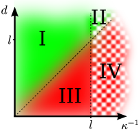
Figure 2: Sketch of the regimes discussed in the main text for the case of comparable screening lengths, $\kappa^{-1}_{1}\sim\kappa^{-1}_{2}$ (denoted by $\kappa^{-1}$). The regimes I and II correspond to effectively decoupled surfaces (studied in Ref. Ostrovsky et al., 2010), while in regimes III and IV intersurface interaction is important. The conductivity corrections in I and III are due to “overscreened” Coulomb interaction. In contrast, in II and IV this type of corrections sets in only in the low-energy regime where the running length scale (i.e. the typical scale $L_{E}$) exceeds the screening length.

In the end of the paper, Sec. VI, we analyze in detail the regions and limits of applicability of our theory with respect to representative experimental setups. In particular, we show that the hierarchy of scales $d\ll l\ll L_{E}$ is realistic.

In order to illustrate the importance of intersurface interaction (i.e. the relevance of the inequality $d\lesssim\kappa_{s}^{-1}$) under realistic conditions, we show in Fig. 3 a dependence of the screening length on the Fermi momentum.

The density of states for the linear (Dirac) spectrum is $\nu(\mu_{s})=k^{(s)}_{F}/2\pi\hbar v_{F}$, where $k^{(s)}_{F}$ is the Fermi wave vector of the $s$-th surface state and $v_{F}$ the Fermi velocity. Therefore

$$\kappa_{s}^{-1}=\frac{1}{\alpha}\frac{1}{k^{(s)}_{F}}.$$ (11)

We introduced the dimensionless parameter $\alpha={e^{2}}/{\epsilon\hbar v_{F}}$ which is the effective coupling constant of the Coulomb interaction and is equal to ${c}/{\epsilon v_{F}}$ times the fine structure constant of quantum electrodynamics. Clearly, $\alpha$ plays the same role as the dimensionless density parameter $r_{s}$ in conventional theories of electrons in parabolic bands. We will assume that the interaction is not too strong, $\alpha\lesssim 1$; otherwise the system may become unstable, see a discussion at the end of Sec. II.3.

The dashed red curve in Fig. 3 represents the lower bound (corresponding to $\alpha=1$) of $\kappa_{s}^{-1}$ as a function of $k^{(s)}_{F}$. The actual value of $\kappa_{s}^{-1}$ for an exemplary case of Bi₂Se₃ (experimental parameters can be found in Table 1 below) is depicted by the blue solid curve. We see that the screening length can by far exceed the thickness of the topological insulator slab. Indeed, the Bi₂Se₃ experiments Wang ; Liu ; Chen et al. (2011); Steinberg are performed on probes of thickness $d\simeq 1-100$ nm. For this material, our assumption of separate gapless surface states (no tunneling) is both numericallyLinder et al. (2009) and experimentallyTaskin et al. (2012) shown to be valid down to $d\simeq 10$ nm (blue horizontal dashed line). Thus, relevant experimental values of $d$ in the experiments of interest range from $d\simeq 10$ nm up to $d\simeq 100$ nm. On the other hand, surface electrons have a maximal Fermi wavevector of $k_{F}\sim 0.1/\text{\AA}$ associated with $\mu=\Delta_{\text{bulk}}=0.3$ eV, see blue vertical dashed line. For the lowest concentration, increase of the screening length is limited by disorder. In this way, we estimate the range of $\kappa_{s}^{-1}$ as 20-200 nm, so that the condition $\kappa_{s}^{-1}>d$ can be easily fulfilled. This is particularly the case for relatively thin films ($d\simeq 10$ nm) and in the vicinity of surface Dirac point.

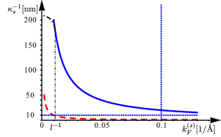
Figure 3: Plot of the single surface screening length $\kappa_{s}^{-1}$. The red curve (large dashes) is the lower bound (corresponding to $\alpha=1$) of the screening length. The solid, blue curve is the screening length for Bi₂Se₃ film with experimental parameters given in Table 1 in Sec.VI.2. For the latter, the required minimal thickness and maximal Fermi momentum are also depicted (dotted blue lines). The disorder-induced regularization of the divergence at small Fermi momentum is schematically represented by the black dot-dashed curve.

The above analysis proves the relevance of the intersurface electron-electron interaction. In fact, in course of this analysis we have made several simplifying assumptions that require certain refinements; we list them for the reader’s benefit. First, in general, the coating material ($\epsilon_{1}$), the topological insulator ($\epsilon_{2}$), and the substrate ($\epsilon_{3}$) are all dielectrica with different dielectric constants $\epsilon_{1}\neq\epsilon_{2}\neq\epsilon_{3}$. In order to determine the exact Coulomb interaction, one has to solve the electrostatic problem of a point charge in such a sandwich structure of dielectrica,Profumo2010 ; Katsnelson2011 ; Carrega et al. (2012) see Appendix B. Second, the long-range Coulomb interaction is accompanied by short-range contributions, which, in particular, induce corrections to the polarization operator which affect the screening length. More precise calculations taking Fermi liquid corrections into account can be found in Section III.6.4 and Appendix C. Finally, we neglected the dependence of the Fermi velocity $v_{F}$ on the chemical potential $\mu_{s}$, see Sec. II.3. However, all these refinements do not modify our conclusion of the importance of interaction between the surface states. We now proceed with presentation of the field-theoretical formalism that will allow us to explore the problem.

II.3 Microscopic Hamiltonian

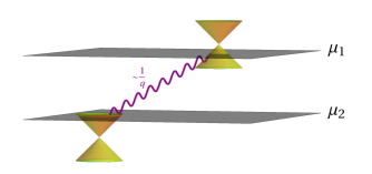
Figure 4: Pictographic representation of the microscopic model: Diffusively propagating surface states at different chemical potentials which interact with each other by means of long-range Coulomb interaction.

The model under consideration is schematically depicted in Fig. 4. It is described in path integral technique

$$\mathcal{Z}=\int\mathcal{D}\left[\bar{\psi},\psi\right]\;e^{-S\left[\bar{\psi},\psi\right]}$$ (12)

by the following microscopic Matsubara action:

$$S\left[\bar{\psi},\psi\right]=\int_{\tau,\textbf{{x}}}\bar{\psi}\left(\partial_{\tau}+\text{H}_{0}+\text{H}_{\rm dis}\right)\psi+S_{\rm int}.$$ (13)

The notation $\int_{\tau,\textbf{{x}}}=\int d^{2}x\int_{0}^{\beta}d\tau$ will be used throughout the article, where, as usual, $\beta=1/T$ is the inverse temperature. If not specified otherwise, we set Boltzmann’s constant, Planck’s constant, and the speed of light $k_{B}=\hbar=c=1$ in the remainder. The fermionic fields $\bar{\psi}\left(\textbf{{x}},\tau\right)=\left(\bar{\psi}^{\uparrow}_{1},\bar{\psi}^{\downarrow}_{1},\bar{\psi}^{\uparrow}_{2},\bar{\psi}^{\downarrow}_{2}\right)$ and $\psi\left(\textbf{{x}},\tau\right)=\left(\psi^{\uparrow}_{1},\psi^{\downarrow}_{1},\psi^{\uparrow}_{2},\psi^{\downarrow}_{2}\right)^{T}$ describe the spinful ($\uparrow,\downarrow$) excitations living on surfaces $s=1$ and $s=2$. The one particle Hamiltonian which characterizes the surface $s$ is

$$\left(\text{H}_{0}+\text{H}_{\rm dis}\right)_{s}=\left(V_{s}(\textbf{{x}})-\mu_{s}\right)\otimes\mathbf{I}_{\sigma}+i(-)^{s}v^{(s)}_{F}\nabla\wedge\vec{\sigma},$$ (14)

where $\mathbf{I}_{\sigma}$ is the unit matrix in spin space and we define $\textbf{{a}}\wedge\textbf{{b}}=a_{x}b_{y}-a_{y}b_{x}$. The disorder potentials $V_{s}\left(\textbf{{x}}\right)$ for two surfaces are assumed to be white-noise distributed and uncorrelated:

$$\left\langle V_{s}(\textbf{{x}})V_{s^{\prime}}(\textbf{{x}}^{\prime})\right\rangle=\frac{\delta\left(\textbf{{x}}-\textbf{{x}}^{\prime}\right)\delta_{ss^{\prime}}}{\pi\nu_{s}\tau_{s}}.$$ (15)

The disorder strengths $1/\pi\nu_{s}\tau_{s}$ may be different for two surfaces.

It is worth emphasizing the following physical implications of this Hamiltonian.

• First, the model (and its analysis below) corresponds to the general case in which the chemical potentials $\mu_{1}$, $\mu_{2}$ and hence the carrier densities of the two surfaces may differ.

• Second, since the disorder potentials are different for two surfaces, no inter-surface diffuson and cooperon modes will arise. Note that the considered model of fully uncorrelated disorder correctly describes the low-energy physics of the majority of experimental setups, even in the presence of moderate inter-surface correlations of disorder. Indeed, any mismatch in chemical potentials and/or disorder configurations leads to an energy gap in the inter-surface soft modes. Two physical regimes are conceivable:

  • almost identical surfaces in almost fully correlated random potentials, $|\mu_{1}-\mu_{2}|\ll 1/\tau_{s}$ and $\left\langle\left[V_{1}(\textbf{{x}})-V_{2}(\textbf{{x}}^{\prime})\right]^{2}\right\rangle\ll\sum_{s=1,2}\left\langle V_{s}(\textbf{{x}})V_{s}(\textbf{{x}}^{\prime})\right\rangle$;

  • all other parameter regimes, when at least one of the conditions in (i) is not fulfilled.

  Our model is designed for the case (ii), where the gap is comparable to the elastic scattering rate and inter- surface soft modes do not enter the diffusive theory at all. It also applies to the case (i) in the ultimate large-scale limit (i.e. at energy scales below the gap). In this case there will be, however, an additional, intermediate regime in the temperature dependence (or AC frequency dependence) which is not considered in our work.

• Third, $\vec{\sigma}$ in Eq.(14) in general does not describe the physical spin. For example, in Bi₂Se₃ structures the effective spin $\sigma$ is determined by a linear combination of real spin and the parity (band) degrees of freedom. The mixing angle depends on how the crystal is cut. Zhang et al. (2012) In this case also the Fermi velocity becomes anisotropic.

• Fourth, because of interaction effects, the true dispersion relation is not linear but contains logarithmic corrections (or more generally is subjected to “ballistic” RG González et al. (2001); Foster and Aleiner (2008); Sheehy and Schmalian (2007)) which leads to dependence of the Fermi velocity on the chemical potential. This is reflected in the notation $v_{F}^{(s)}\equiv v_{F}(\mu_{s})$.

• Similarly, also the strength of the disorder may be substantially different for both surfaces, so that the (quantum) mean free times $\tau_{s}$ are considered as two independent input parameters. This is primarily because the vicinity to the substrate or, respectively, to the coating material makes the impurity concentration on both surfaces a priori different. In addition, $\tau_{s}$ acquire renormalization corrections, leading to a logarithmic dependence on $\mu_{s}$. Aleiner and Efetov (2006); Ostrovsky et al. (2006); Schuessler et al. (2009); Foster and Aleiner (2008)

• The (pseudo-)spin texture on the top and bottom surfaces is opposite (denoted by the factor $(-)^{s}$).

• Finally, in some materials (in particular, in Bi₂Te₃), the Dirac cone is strongly warped. We neglect the warping as it does not affect the main result of this paper, namely the (universal) RG equations. Recently,Adroguer et al. (2012) it has been shown that warping only influences the dephasing length (i.e., the lengthscale at which the RG flow is stopped).

The interaction is mediated by the Coulomb potential, see Eq. (4) and Appendix B. With the definition $\rho_{s}\left(\tau,\textbf{{x}}\right)=\bar{\psi}_{s}\left(\tau,\textbf{{x}}\right)\psi_{s}\left(\tau,\textbf{{x}}\right)$ the corresponding contribution to the action is given by

$$S_{\rm int}=\frac{1}{2}\sum_{ss^{\prime}}\int_{\tau,\textbf{{x}},\textbf{{x}}^{\prime}}\rho_{s}\left(\tau,\textbf{{x}}\right)U_{0,ss^{\prime}}\left(|\textbf{{x}}-\textbf{{x}}^{\prime}\right|)\rho_{s^{\prime}}\left(\tau,\textbf{{x}}^{\prime}\right).$$ (16)

For equal surfaces ($v_{F}^{(1)}=v_{F}^{(2)}$), a simple rescaling of equations (13) and (16) shows that the effective coupling to the Coulomb interaction is $\alpha$. It can, in general, become of the order of unity. Since the perturbation theory is insufficient in such a case, we adopt the more general, yet phenomenological, Fermi liquid theory to access the behavior for energies down to the elastic scattering rates $\tau^{-1}_{1,2}$, see Sections III.6.3, III.6.4 and Appendix C). This (clean) Fermi liquid theory will then be a starting point for the interacting diffusive problem at energies below the elastic scattering rate.

If the interaction becomes too strong, it might in principle drive the system into a phase with spontaneously broken symmetry.SitteRoschFritz2013 Examples are the Stoner instability Peres et al. (2005) as well as more exotic phenomena such as topological exciton condensation, Seradjeh et al. (2009) which is specific to 3D TI thin films. Throughout our analysis, we assume that the system is not in a vicinity of such an instability. To our knowledge, this assumption is consistent with all transport experiments on 3D TI slabs addressed in this work.

III Sigma-model description

We are interested in the low-energy (low-temperature, long-length-scale) physics of the 3D TI problem defined by Eqs. (1) and (2). This physics is controlled by coupled diffuson and cooperon modes. In this Section we derive the effective field theory – diffusive non-linear $\sigma$ model – that describes the system in this regime.

III.1 Symmetries of the action

The structure of the effective low-energy theory, the diffusive NL$\sigma$M, is controlled by symmetries of the microscopic action. The information about other microscopic details enters the theory only via the values of the coupling constants. We thus begin by analyzing symmetries of the problem.

First, our system obeys the time reversal symmetry $H=\sigma_{y}H^{T}\sigma_{y}$. Second, we assume no intersurface tunneling, i.e., the particle number is conserved in each surface separately. This implies invariance of the action with respect to $\mathbf{U}(1)\times\mathbf{U}(1)$ transformations (global in space and time).

The presence of Coulomb interaction promotes the $\mathbf{U}(1)$ symmetry in the total-density channel, $\rho_{1}+\rho_{2}$, to transformations which are local in time but global in space. In other words, rotations of fermionic fields, $\bar{\psi}_{s}\left(\tau,\textbf{{x}}\right)\to\bar{\psi}_{s}\left(\tau,\textbf{{x}}\right)\exp{[-i\chi_{s}(\tau)]}$, $\psi_{s}\left(\tau,\textbf{{x}}\right)\to\exp{[i\chi_{s}(\tau)]}\psi_{s}\left(\tau,\textbf{{x}}\right)$, with equal phases $\chi_{1}\left(\tau\right)=\chi_{2}\left(\tau\right)$ leave the action (13) invariant. This is a special case of “$\mathcal{F}$-invariance” Pruisken et al. (1999) and has important consequences for the present problem. The $\mathcal{F}$-invariance (it is intimately linked to gauge invariance) generally states that in each channel with long-range interaction, time-dependent but spatially constant $\mathbf{U}(1)$ rotations are symmetries of the action. In our problem, as it follows from the $q\to 0$ limit of the Coulomb interaction:

$$\underline{U}\left(\textbf{{q}}\right)\stackrel{{\scriptstyle q\rightarrow 0}}{{\propto}}\frac{1}{q}\left(\begin{array}[]{cc}1&1\\ 1&1\end{array}\right),$$ (17)

only the interaction between the total densities is long-ranged. The structure of Eq. (17) remains true also in the case of asymmetric dielectric environment, see Appendix C.4.

To make the time-reversal symmetry explicit, we define particle-hole bispinors by combining $\psi$ and $\bar{\psi}$ fields. Efe (1980); Belitz and Kirkpatrick (1994) In the momentum space the bispinors read

$$\Phi_{n}\left(\textbf{{k}}\right)=\frac{1}{\sqrt{2}}\left(\begin{array}[]{c}\bar{\psi}_{n}\left(-\textbf{{k}}\right)^{T}\\ i\sigma_{y}\psi_{n}\left(\textbf{{k}}\right)\end{array}\right)$$ (18)

and

$$\bar{\Phi}_{n}\left(\textbf{{k}}\right)=\left[C\Phi_{n}\left(-\textbf{{k}}\right)\right]^{T}\text{ with }C=i\sigma_{y}\tau_{x},$$ (19)

where $n$ is the index associated to the fermionic Matsubara frequency $i\epsilon_{n}$, and $\tau$ matrices act in the particle-hole space. This allows us to rewrite the one-particle Hamiltonian as

$$S^{\rm free}=-\sum_{n}\int_{\textbf{{k}}}\bar{\Phi}_{n}\left(\textbf{{k}}\right)\left(i\epsilon_{n}-H^{T}\left(-\textbf{{k}}\right)\right)\Phi_{n}\left(\textbf{{k}}\right).$$ (20)

It is convenient to perform a rotation of bispinors

$$\eta=\sqrt{\tau_{x}}\Phi,$$ (21)

where $\sqrt{\tau_{x}}=e^{-i\pi/4}(\mathbf{I}_{\tau}+i\tau_{x})/\sqrt{2}$. The free action then takes the form

$$S^{\rm free} = -\sum_{s}\int_{\textbf{{x}}}\eta^{T}_{s}\Big{\{}\left[i\hat{\epsilon}-V_{s}+\mu_{s}\right]\left(-i\sigma_{y}\right)$$ (22)

$$+ \left.(-)^{s+1}v^{(s)}_{F}\left(\partial_{x}-i\partial_{y}\sigma_{z}\right)\right\}\eta_{s}.$$ (23)

The Matsubara frequency summation is incorporated into the scalar product $\eta^{T}\left(\dots\right)\eta$. In these notations, $\hat{\epsilon}$ is a diagonal matrix in the Matsubara space consisting of entries $\epsilon_{n}$.

In order to perform the average over disorder, we replicate the theory $N_{R}$ times. Furthermore, in order to implement the $\mathbf{U}\left(1\right)$-gauge invariance in the framework of the NL$\sigma$M, we apply a double cutoff truncation procedure with $N_{M}\ll N^{\prime}_{M}$ for the Matsubara frequencies.Pruisken et al. (1999) Here $N^{\prime}_{M}$ and $N_{M}$ are the numbers of retained Matsubara harmonics for fast (electrons of the original theory) and slow (diffusons and cooperons of the NL$\sigma$M) degrees of freedom, respectively. As a consequence, $\eta$ becomes a $\left(2_{s}\times 2_{\sigma}\times 2_{\tau}\times 2N^{\prime}_{M}\times N_{R}\right)$-dimensional Grassmannian vector field. Except for the frequency term, the free action (23) is manifestly invariant under global orthogonal rotations of the kind

$$\eta_{s}\rightarrow\left(O_{s}\otimes\mathbf{I}_{\sigma}\right)\eta_{s}\text{ with }O_{s}\in\mathbf{O}\left(2_{\tau}\times 2N^{\prime}_{M}\times N_{R}\right).$$ (24)

Since the surfaces are fully decoupled in the absence of interactions, the rotations $O_{1}$ and $O_{2}$ of the fields corresponding to the top and bottom surfaces are completely independent.

III.2 Quasiclassical conductivity

To obtain the quasiclassical conductivity, we first find the fermionic self-energy within the self-consistent Born approximation (SCBA):

$$\Sigma^{s}_{n}=\frac{-2i\sigma_{y}}{\pi\nu_{s}\tau_{s}}\left\langle\eta_{\textbf{{x}},s}\eta_{\textbf{{x}},s}^{T}\right\rangle_{\text{SCBA}}.$$ (25)

Here $\left\langle\dots\right\rangle_{\text{SCBA}}$ denotes the self-consistent treatment, i.e. a shift $\mu_{s}\rightarrow\mu_{s}+\Sigma^{s}_{n}$ in the fermionic propagator. Equation (25) yields for the imaginary part of the self-energy ${\rm Im}(\Sigma^{s}_{n})=(i/2\tau_{s})\text{sgn}(n)$. The quasiclassical Drude DC conductance of the non-interacting problem in the absence of a magnetic field is

$$\sigma^{D}_{s}=2\pi\nu_{s}D_{s}\frac{e^{2}}{h},$$ (26)

with $D_{s}=(v^{(s)}_{F})^{2}\tau_{s}$. Note that the transport time is twice the quantum mean free time $\tau_{s}$. In the diagrammatic language, this is a consequence of vertex corrections.

III.3 Fermionic currents and bosonization rules

To derive the NL$\sigma$M, we use the method of non-Abelian bosonization. Witten (1984); Nersesyan et al. (1994, 1995); Altland et al. (2002); Altland (2006) An advantage of this approach is that non-trivial topological properties of the Dirac fermions are translated into the field theory in a particularly transparent way.

In the first step, the kinetic term (Sec. III.4) is bosonized. Subsequently, we bosonize also the terms induced by the chemical potential, disorder and frequency (Sec. III.5). Since only interaction couples the two surfaces, we omit the surface index $s$ in Sec. III.4 and Sec. III.5. This index is restored later in Sec. III.6 where the interaction is included.

Local left ($\eta_{\uparrow}\rightarrow O_{L}\eta_{\uparrow}$) and right ($\eta_{\downarrow}\rightarrow O_{R}\eta_{\downarrow}$) rotations define the left and right currents. The bosonization rules for these currents as well as for the mass term are

$$j_{+}=v_{F}\eta_{\uparrow}\eta_{\uparrow}^{T} \leftrightarrow\frac{1}{8\pi}\left(O\partial_{+}O^{T}\right),$$ (27a)

$$j_{-}=v_{F}\eta_{\downarrow}\eta_{\downarrow}^{T} \leftrightarrow\frac{1}{8\pi}\left(O^{T}\partial_{-}O\right),$$ (27b)

$$\eta_{\uparrow}\eta_{\downarrow}^{T} \leftrightarrow i\lambda O,$$ (27c)

where $\partial_{\pm}=\partial_{x}\pm i\partial_{y}$. The energy scale $\lambda$ is of the order of the ultraviolet (UV) cutoff and is introduced here for dimensional reasons; see Sec. III.5.1 and IV.2 for a discussion of its physical meaning. Note that in general, the UV cutoff is different for the top and bottom surfaces, $\lambda_{1}\neq\lambda_{2}$. Further, $O$ is an orthogonal $\left(2_{\tau}\times 2N^{\prime}_{M}\times N_{R}\right)\times\left(2_{\tau}\times 2N^{\prime}_{M}\times N_{R}\right)$ matrix field. Below we will need the following constant matrices in this space

$$\Lambda^{\tau_{1}\tau_{2};\alpha\beta}_{nm} = \text{sgn}\left(n\right)\delta^{\tau_{1}\tau_{2}}\delta^{\alpha\beta}\delta_{nm},$$

$$\hat{\eta}^{\tau_{1}\tau_{2};\alpha\beta}_{nm} = n\delta^{\tau_{1}\tau_{2}}\delta^{\alpha\beta}\delta_{nm},$$ (28)

$$\left(I^{\alpha_{0}}_{n_{0}}\right)^{\tau_{1}\tau_{2};\alpha\beta}_{nm} = \delta^{\tau_{1}\tau_{2}}\delta^{\alpha_{0}\alpha}\delta^{\alpha_{0}\beta}\delta_{n-m,n_{0}}.$$

Here and throughout the paper we use a convention that $\alpha,\beta\in\left\{0,N_{R}\right\}$ denote replicas and $m,n\in\left\{-N^{\prime}_{M},\dots,N^{\prime}_{M}-1\right\}$ Matsubara indices. The double cutoff regularization scheme Pruisken et al. (1999) prescribes that matrices $O$ have non-trivial matrix elements $O_{nm}$ only for low-energy excitations $n,m\in\left\{-N_{M},\dots,N_{M}-1\right\}$ and stay equal to the origin $O_{0}$ of the $\sigma$ model manifold outside this low-energy region. As explained below, $O_{0}=\Lambda$.

III.4 Bosonization of the kinetic part

The kinetic part of (23) is nothing but the Euclidean counterpart of the model considered in Ref. Witten, 1984. Upon non-Abelian bosonization it yields the Wess-Zumino-Novikov-Witten (WZNW) action

$$S_{\rm WZNW}=\int_{\textbf{{x}}}\frac{1}{16\pi}\text{tr}\nabla O\nabla O^{-1}+\frac{i}{24\pi}\Gamma_{WZ},$$ (29)

where $\Gamma_{WZ}$ is the Wess-Zumino (WZ) term

$$\Gamma_{WZ}=\int_{\textbf{{x}},w}\epsilon_{\mu\nu\rho}\text{tr}\left[\left(\tilde{O}^{-1}\partial_{\mu}\tilde{O}\right)\left(\tilde{O}^{-1}\partial_{\nu}\tilde{O}\right)\left(\tilde{O}^{-1}\partial_{\rho}\tilde{O}\right)\right],$$ (30)

where $\epsilon_{\mu\nu\rho}$ denotes the Levi-Civita symbol. The definition of the WZ term involves an auxiliary coordinate $w\in\left[0,1\right]$ and smooth fields $\tilde{O}\left(\textbf{{x}},w\right)$ satisfying $\tilde{O}\left(\textbf{{x}},w=0\right)={\rm const}$ and $\tilde{O}\left(\textbf{{x}},w=1\right)=O\left(\textbf{{x}}\right)$. As a result the compactified two-dimensional coordinate space $\mathbb{R}^{2}\cup\left\{\infty\right\}\simeq\mathbb{S}^{2}$ is promoted to the solid 3-ball $\mathbb{B}^{3}$ (i.e., the “filled” sphere).

III.5 Free NL$\sigma$M of class AII

III.5.1 Disorder, frequency, and the chemical potential

The action (29) is the bosonized counterpart of the second (proportional to velocity) term of the microscopic action (23). Let us now consider the first term in Eq. (23) which carries information about the chemical potentials, frequency and random potential.

Bosonization of the terms with frequency and the chemical potential in the microscopic action (23) yields

$$\delta S=2\int_{\textbf{{x}}}\text{tr}\left[\left(i\hat{\epsilon}+\mu\right)\eta_{\uparrow}\eta_{\downarrow}^{T}\right]\leftrightarrow-2\lambda\int_{\textbf{{x}}}\text{tr}\left(\hat{\epsilon}-i\mu\right)O.$$ (31)

Upon disorder averaging and bosonization, the term with random potential provides the following contribution to the field theory:

$$\delta S_{\textrm{dis}} =-\frac{1}{\pi\nu\tau}\int_{\textbf{{x}}}\left(\text{tr}\eta_{\uparrow}\eta_{\downarrow}^{T}\right)^{2}+\frac{1}{\pi\nu\tau}\int_{\textbf{{x}}}\text{tr}(\eta_{\uparrow}\eta_{\downarrow}^{T})^{2}$$

$$\leftrightarrow\frac{\lambda^{2}}{\pi\nu\tau}\int_{\textbf{{x}}}\left(\text{tr}O\right)^{2}$$

$$+\frac{\lambda^{2}}{2\pi\nu\tau}\int_{\textbf{{x}}}\text{tr}\left(O^{T}-O\right)^{T}\left(O^{T}-O\right).$$ (32)

As we see, disorder induces mass terms for $O$-matrices. Both mass terms in Eq. (32) are strictly non-negative. Therefore, they are minimized by arbitrary traceless symmetric orthogonal matrix. It is convenient to choose the specific saddle-point solution as

$$O=\Lambda.$$ (33)

This saddle-point solution coincides with the SCBA. Indeed, Eq. (25) can be written as

$$\frac{i}{2\tau}\Lambda{\otimes\textbf{1}}_{\sigma} =\frac{2}{\pi\nu\tau}\left\langle\left(\begin{array}[]{cc}-\eta_{\downarrow}\eta_{\uparrow}^{T}&-\eta_{\downarrow}\eta_{\downarrow}^{T}\\ \eta_{\uparrow}\eta_{\uparrow}^{T}&\eta_{\uparrow}\eta_{\downarrow}^{T}\end{array}\right)\right\rangle_{\text{SCBA}}$$ (36)

$$\leftrightarrow\frac{2}{\pi\nu\tau}\left\langle\left(\begin{array}[]{cc}i\lambda O^{T}&\frac{-1}{8\pi v_{F}}O^{T}\partial_{-}O\\ \frac{1}{8\pi v_{F}}O\partial_{+}O^{T}&i\lambda O\end{array}\right)\right\rangle.$$ (39)

It is solved by the saddle-point solution (33) provided the auxiliary UV energy scale $\lambda$ introduced in Eq. (27) is related to the density of states (i.e., to the chemical potential),

$$\lambda=\frac{\pi\nu}{4}=\frac{|\mu|}{8v_{F}^{2}}.$$ (40)

We will rederive this relation from a different viewpoint below, see Sec. IV.2.

Equation (33) is not the only solution of the saddle point equation. It is easy to see that rotations

$$O\rightarrow O^{T}_{\text{soft}}OO_{\text{soft}},\;O_{\text{soft}}\in\mathbf{G}=\mathbf{O}\left(2_{\tau}\times 2N_{M}\times N_{R}\right)$$ (41)

leave the mass term unaffected. On the other hand, the saddle-point $O=\Lambda$ is invariant under rotations from a smaller group, $O_{\text{soft}}\in\mathbf{K}=\mathbf{O}\left(2_{\tau}\times N_{M}\times N_{R}\right)\times\mathbf{O}\left(2_{\tau}\times N_{M}\times N_{R}\right)$. This can be understood as a breakdown of symmetry $\mathbf{G}\to\mathbf{K}$. We thus obtain a non-trivial manifold of saddle-points annihilating the mass term. Allowing for a slow variation of $O_{\text{soft}}$ and restricting other terms in the action to this manifold, we will obtain the NL$\sigma$M action.

III.5.2 Free NL$\sigma$M with $\mathbb{Z}_{2}$ topological term

As we have just discussed, we keep only the soft modes

$$Q=O^{T}_{\text{soft}}\Lambda O_{\text{soft}}\text{ with }O_{\text{soft}}\in\mathbf{G}.$$ (42)

The subscript ${}_{\text{soft}}$ will be omitted in the remainder. The NL$\sigma$M manifold ${\cal M}=\mathbf{G}/\mathbf{K}$. We also rename the coupling constants according to the conventional notation of diffusive NL$\sigma$Ms and restore the surface index $s$,

$$S^{\rm free}=\sum_{s}\int_{\textbf{{x}}}\frac{\sigma_{s}}{16}\text{tr}\left(\nabla Q_{s}\right)^{2}-2\pi Tz_{s}\text{tr}\left[\hat{\eta}Q_{s}\right]+iS^{(\theta)}_{s}.$$ (43)

As will become clear from linear response theory (Sec. III.7.3), $\sigma_{s}$ measures the DC conductivity of surface $s$ (in units $e^{2}/h$). Its bare value is the Drude conductance depending on the chemical potential $\mu_{s}$, as can be directly verified, see Appendix A.1. The coupling constants $z_{s}$ determine the renormalization of the specific heat.

The non-trivial second homotopy group of the NL$\sigma$M manifold $\pi_{2}({\cal M})=\mathbb{Z}_{2}$ allows for topological excitations (instantons), similarly to the QHE theory. A crucial difference is that in the QHE case the second homotopy group is $\mathbb{Z}$, so that any integer topological charge (number of instantons) is allowed. Contrary to this, in the present case any configuration of an even number of instantons can be continuously deformed to the trivial, constant vacuum configuration. Therefore, the theta term $S^{(\theta)}_{s}$ appearing in (43) only distinguishes between an even ($S^{(\theta)}_{s}=0\;\text{mod}\;2\pi$) and odd ($S^{(\theta)}_{s}=\pi\;\text{mod}\;2\pi$) number of instantons.

Such a $\mathbb{Z}_{2}$ theta term $S^{(\theta)}$ does not appear in the case of usual metals with strong spin-orbit coupling; it results from the Dirac-fermion nature of carriers and is a hallmark of topologically protected metals (in our case, the surface of a topological insulator). The topological term flips the sign of the instanton effects (as compared to the case of a usual metal with spin-orbit interaction) from localizing to delocalizing. Thus, the theta term translates the protection against Anderson localization into the NL$\sigma$M approach.

We are now going to show that $S^{(\theta)}_{s}$ is nothing but the WZ term (obtained from non-Abelian bosonization) restricted to the smaller symmetry group:

$$S^{(\theta)}_{s}=\frac{1}{24\pi}\left.\Gamma_{WZ,s}\right|_{\tilde{O}_{s}\left(\textbf{{x}},w=1\right)=Q_{s}\left(\textbf{{x}}\right)=Q_{s}^{T}\left(\textbf{{x}}\right)}.$$ (44)

Note that, since the second homotopy group of the NL$\sigma$M manifold is non-trivial, the definition of the WZ term requires that away from $w=1$ the extended fields can take values in the big orthogonal group $\mathbf{G}$.

To show that Eq. (44) is indeed the $\mathbb{Z}_{2}$ theta-term, we proceed in the same way as was recently done for symmetry class CII.König et al. (2012) First of all, it is straightforward to check that $S^{(\theta)}_{s}$ is invariant under small variations of the sigma-model field, $Q_{s}\rightarrow Q^{\prime}_{s}=Q_{s}+\delta Q_{s}$ ($Q_{s}^{\prime 2}=\mathbf{1}=Q_{s}^{2}$). Thus, $S^{(\theta)}_{s}$ only depends on the topology of the field configuration. This immediately implies that it is zero in the topologically trivial sector. In order to proof that $S^{(\theta)}_{s}$ also returns the correct value $S^{(\theta)}_{s}=\pi\;(\text{mod}\;2\pi)$ in the topologically non-trivial sector, it is sufficient to insert a single instanton into $S^{(\theta)}_{s}$. Instantons are field configurations that per definition can not be continuously deformed into the vacuum configuration. Introducing the third dimension and allowing the field to take values in the entire orthogonal group we can continuously shrink the instanton in the $w=1$ sphere to the constant at $w=0$. A necessary condition for this untwisting to happen is that for some subinterval of $\left(0,1\right)$ the field leaves the NL$\sigma$M manifold for the larger orthogonal group. A direct calculation shows that the group volume covered while untwisting indeed yields the value $iS^{(\theta)}_{s}=i\pi$, see Appendix A.2).

There have been alternative derivations of the $\mathbb{Z}_{2}$ term before Ryu et al. (2007); Ostrovsky et al. (2007). Viewing this theta term as a symmetry-broken WZ-term, Eq. (44), yields a local expression for it and implies the following advantages. First, this form is very useful for understanding the crossover between 3D topological insulators of class DIII and AII. Second and more importantly, an analysis of response of the system to an external electric field requires coupling of the diffusive matter fields to $\mathbf{U}(1)$ gauge potentials. In particular, one should gauge the topological term, which can be done in a standard way by using a local expression for it. We will show in Section III.7.4 that such a procedure yields the correct linear response theory for the anomalous quantum Hall effect of Dirac fermions.

In addition to a non-trivial second homotopy group $\pi_{2}$, the sigma model manifold of the class AII possesses also a non-trivial first homotopy group, $\pi_{1}({\cal M})=\mathbb{Z}_{2}$. For this reason, the RG flow in 2D systems of class AII (as well as in other classes with a non-trivial $\pi_{1}$ group, namely AIII, BDI, CII, and DIII) is affected by vortices, as was shown in Ref. König et al., 2012. In the case of AII (and DIII) class these are $\mathbb{Z}_{2}$ vortices,König et al. (2012) i.e., a vortex is identical to an anti-vortex. In a recent work Fu and Kane (2012) it was argued that such vortices are crucial for establishing localization in the class AII. Conversely, the robustness of a non-localized state on the surface of a weak topological insulator and of the critical state separating 2D trivial and topological insulator were explained by vanishing of the corresponding fugacity.

On the surface of a strong 3D TI, the effect of vortices is erased by the $\mathbb{Z}_{2}$ topological term, in the same way as argued previouslyKönig et al. (2012) for the case of the symmetry class CII. Specifically, due to the $\mathbb{Z}_{2}$ theta term, the vortices acquire an internal degree of freedom which, upon averaging, annihilates the contribution of vortices to renormalization. For this reason, the vortices need not be taken into account in the present context.

III.6 Interacting NL$\sigma$M

In the previous subsection we have derived the diffusive non-linear sigma model for non-interacting particles. The next step is to include the electron-electron interactions.

III.6.1 Interacting Fermi gas

We concentrate first on the case of a weak Coulomb interaction ($\alpha\ll 1$). At length scales larger than the screening length the interaction is effectively pointlike:

$$S_{\rm int}=\frac{T}{2}\sum_{m,\alpha;ss^{\prime}}\int_{\textbf{{x}}}\text{tr}{\left(I_{m}^{\alpha}\psi_{s}\bar{\psi}_{s}\right)}U^{q}_{ss^{\prime}}{\left(I_{-m}^{\alpha}\psi_{s^{\prime}}\bar{\psi}_{s^{\prime}}\right)}$$ (45)

where $U^{q}_{ss^{\prime}}$ is the “overscreened” Coulomb interaction matrix i.e., the $q\rightarrow 0$ limit of Eq. (9) (for its generalization in case of an asymmetric dielectric environment, see Appendix B). We use the bosonization rule

$$\text{tr}I_{m}^{\alpha}\psi_{s}\bar{\psi}_{s} =\text{tr}I_{m}^{\alpha}\left(1-\tau_{y}\right)\eta_{s,\uparrow}\eta_{s,\downarrow}^{T}-\text{tr}I_{m}^{\alpha}\left(1-\tau_{y}\right)\eta_{s,\downarrow}\eta_{s,\uparrow}^{T}$$

$$\leftrightarrow i\lambda\left[\text{tr}I_{m}^{\alpha}\left(1-\tau_{y}\right)\left(O_{s}+O_{s}^{T}\right)\right].$$ (46)

When disorder is introduced, the matrices $O$ become restricted to the sigma-model manifold ${\cal M}$, and we obtain

$$S_{\rm int}{=}-\lambda^{2}8T\sum_{m,\alpha;ss^{\prime}}\int_{\textbf{{x}}}{\text{tr}\left[J_{-m}^{\alpha}Q_{s}\right]}U^{q}_{ss^{\prime}}{\text{tr}\left[J_{m}^{\alpha}Q_{s^{\prime}}\right]}.$$ (47)

Here we have defined $J_{n}^{\alpha}=I_{n}^{\alpha}\frac{1+\tau_{y}}{2}$. As has been already emphasized, we want to treat the general case of strong interactions up to $\alpha\sim 1$. Therefore, in the following (and in more detail in Appendix C), we present the Fermi liquid (FL) treatment of strongly interacting surface states of a thin 3D TI film.

III.6.2 Effective spinless theory

One of the most striking peculiarities of the surface states of 3D topological insulators is their Rashba-like kinetic term. As a consequence, spin and momentum are locked in a manner visualized in Fig. 5. Such states are called helical; one associates helicity eigenvalues $+1$ ($-1$) with states with positive (respectively, negative) kinetic energy. As has been stated above, we will be interested in the low energy regime $E\ll|\mu_{1,2}|$. Hence, at each of the surfaces only one type of helical states represents dynamical low energy degrees of freedom, while the other one is suppressed by a mass $\approx 2|\mu_{1,2}|$. Therefore, we project onto the appropriate helicity eigenstate of each surface using the following projection operator

$$\mathcal{P}_{s}=|\mu_{s},\textbf{{p}}\rangle\langle\mu_{s},\textbf{{p}}|\text{ with }|\mu_{s},\textbf{{p}}\rangle=\frac{1}{\sqrt{2}}\left(\begin{array}[]{c}1\\ i\text{sgn}\mu_{s}\;e^{i\phi(\textbf{{p}})}\end{array}\right),$$ (48)

where we have defined the polar angle $\phi$ of the momentum, $p_{x}\equiv|\textbf{{p}}|\cos\phi$ and $p_{y}\equiv|\textbf{{p}}|\sin\phi$. The clean single-particle action becomes effectively spinless:

$$S^{(s)}_{0}=-\sum_{s}\int_{\textbf{{p}}}\bar{\zeta}_{s}\left(\textbf{{p}}\right)\left[i\hat{\epsilon}+\text{sgn}\left(\mu_{s}\right)\left(|\mu_{s}|-v_{F}^{s}|\textbf{{p}}|\right)\right]\zeta_{s}\left(\textbf{{p}}\right),$$ (49)

where $\zeta_{s}$, $\bar{\zeta}_{s}$ are the fields associated with the helicity eigenstates, $\zeta_{s}=\langle\mu_{s},\textbf{{p}}|\psi_{s}$ and $\bar{\zeta}_{s}=\bar{\psi}_{s,\sigma}|\mu_{s},\textbf{{p}}\rangle$.

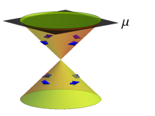
Figure 5: Schematic representation of the Dirac cone and the strong Rashba spin orbit coupling. If the chemical potential (black plane) is large compared to the typical energy scale $E$ (e.g., temperature), only one kind of helical states can take part in the dynamics.

III.6.3 Scattering channels

In the presence of a Fermi surface, the electron-electron interaction at low energies decouples into separate scattering channels defined by small energy-momentum transfer and by the tensor structure in the surface space:

$$S_{\rm int}=-\frac{T}{2}\int_{P_{1},P_{2},K}\sum_{\alpha}\left[\mathcal{O}^{IA}_{0+1}+\mathcal{O}^{IA}_{2}+\mathcal{O}^{IA}_{c}\right]$$ (50)

with

$$\mathcal{O}^{IA}_{0+1} = \sum_{s_{1}s_{2}}\left[\bar{\zeta}^{\alpha}_{s_{1}}\left(P_{1}\right)\zeta^{\alpha}_{s_{1}}\left(P_{1}+K\right)\right]$$ (51)

$$\times\Gamma^{0+1,q}_{s_{1},s_{2};\hat{p}_{1},\hat{p}_{2}}\left[\bar{\zeta}^{\alpha}_{s_{2}}\left(P_{2}\right)\zeta^{\alpha}_{s_{2}}\left(P_{2}-K\right)\right],$$

$$\mathcal{O}^{IA}_{2} = \sum_{s_{1}s_{2}}\left[\bar{\zeta}^{\alpha}_{s_{1}}\left(P_{2}\right)\zeta^{\alpha}_{s_{1}}\left(P_{1}+K\right)\right]$$ (52)

$$\times\Gamma^{2,q}_{s_{1},s_{2};\hat{p}_{1},\hat{p}_{2}}\left[\bar{\zeta}^{\alpha}_{s_{2}}\left(P_{1}\right)\zeta^{\alpha}_{s_{2}}\left(P_{2}-K\right)\right],$$

and

$$\mathcal{O}^{IA}_{c} = \sum_{s_{1}s_{2}}\left[\bar{\zeta}^{\alpha}_{s_{1}}\left(P_{2}\right)\zeta^{\alpha}_{s_{1}}\left(-P_{1}+K\right)\right]$$ (53)

$$\times\Gamma^{c,q}_{s_{1},s_{2};\hat{p}_{1},\hat{p}_{2}}\left[\bar{\zeta}^{\alpha}_{s_{2}}\left(-P_{2}+K\right)\zeta^{\alpha}_{s_{2}}\left(P_{1}\right)\right].$$

Here the capital letters denote 2+1 momenta. The smallness of $K=\left(\omega_{m},\textbf{{q}}\right)$ means that the following conditions hold $\left(\omega_{m},|\textbf{{q}}|\right)\ll\left(|\mu_{s}|,p^{(s)}_{F}\right)$ for both $s=1,2$. We emphasize that all “Dirac factors” of 3D surface electrons are included in the angular dependence of the scattering amplitudes (subscripts $\Gamma_{\hat{p}_{1},\hat{p}_{2}}$).

We refer to the three scattering channels as small angle scattering channel ($\Gamma^{0+1}$), large angle scattering channel ($\Gamma^{2}$), and the Cooper channel ($\Gamma^{c}$). The quantities entering Eq. (50) are the static limit of the corresponding scattering amplitude, $\Gamma\left(\omega_{m}=0,\textbf{{q}}\right)$. They already include static screening and do not acquire any tree-level corrections due to disorder. Finkelstein (1990); Finkel’stein (2010) Exemplary diagrams are given in figures 6 – 9. There, the small angle scattering amplitude is subdivided into its one Coulomb line reducible part ($\Gamma^{0}$) and irreducible part ($\Gamma^{1}$) such that

$$\Gamma^{0+1}=\Gamma^{0}+\Gamma^{1}.$$ (54)

The irreducible part $\Gamma^{1}$ also includes the short range interaction induced by the finite thickness of the 3D TI film (see Appendix B and C.6).

For the short-range interaction amplitudes ($\Gamma^{1}$, $\Gamma^{2}$, $\Gamma^{c}$), the static limit coincides with the “q-limit” $\Gamma^{q}=\lim_{q\rightarrow 0}\Gamma\left(\omega_{m}=0,\textbf{{q}}\right)$, see also Appendix C. It should be kept in mind that for the one-Coulomb-line-reducible part $\Gamma^{0}$ (it is long-ranged) the “q-limit” $\Gamma^{0,q}$ is only a valid approximation if the mean free path $l$ exceeds the screening length. This applies to most realistic situations. (In the opposite case $\Gamma^{0}$ is parametrically small. On top of this, the $q$-dependence of the Coulomb potential implies a strong scale dependence of both conductivity corrections and the interaction amplitude until the running scale reaches the screening length at which $\Gamma^{0}\approx\Gamma^{0,q}$ is again justified.)

We conclude this section with a side remark concerning the topological exciton condensation. Seradjeh et al. (2009) In order to find the conventional pole structure of the FL Green’s functions for the case $\text{sgn}(\mu_{s})=-1$ one needs to transpose the bilinear form in action (49) and swap the notation $\zeta_{s}\left(\epsilon_{n}\right)\leftrightarrow\bar{\zeta}_{s}\left(-\epsilon_{n}\right)$. If $\text{sgn}(\mu_{1}\mu_{2})=-1$, this interchange of notations obviously happens in only one surface. In this case, the large-angle scattering amplitude $\Gamma^{2}_{12}$ and the Cooper-channel amplitude $\Gamma^{c}_{12}$ are interchanged. Even though this procedure illustrates the analogy between exciton condensation (divergence in $\Gamma^{2}_{12}$) and Cooper instability (divergence in $\Gamma^{c}_{12}$), in the following we choose to keep our original notation of $\zeta_{s}$ and $\bar{\zeta}_{s}$ also in the case of $\mu_{s}<0$.

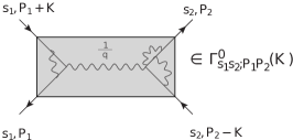
Figure 6: An example of contribution to a one Coulomb-line reducible small angle scattering amplitude. Independently of $\text{sgn}\left(\mu_{s}\right)$, ingoing arrows denote fields $\zeta_{s}$, outgoing arrows $\bar{\zeta}_{s}$.

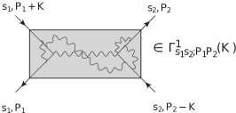
Figure 7: An example of contribution to a one-Coulomb-line irreducible small-angle scattering amplitude.

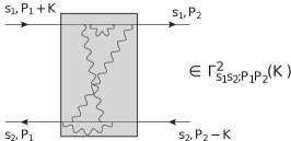
Figure 8: An example of contribution to a large-angle scattering amplitude.

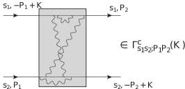
Figure 9: An example of contribution to a scattering amplitude in the Cooper channel.

III.6.4 Clean Fermi liquid theory

A systematic treatment of the scattering amplitudes involves the field-theory of the FLNozieres and Luttinger (1962); Abrikosov et al. (1963); Lifshitz et al. (1980) (see Appendix C.) It is valid down to energy scales $\sim\tau^{-1}_{1,2}$ and therefore constitutes the starting point for the effective diffusive theory at lower energies, $T\ll\tau^{-1}_{1,2}$.

In contrast to the Green’s function of the free theory, in the FL the exact electronic propagator contains both a singular and a regular part. The singular part (“quasiparticle pole”) includes a renormalized dispersion relation and its residue is no more equal to unity but rather is $a_{s}\in\left(0,1\right)$. As usual in the context of disordered FLs,Finkelstein (1990) we absorb the quasiparticle residue by rescaling the fermionic fields and redefining the scattering amplitude.

The conservation of the particle number separately in each of the two surfaces leads to the following Ward identities:

$$\Pi^{\omega}_{s_{1},s_{2}}\equiv\lim_{\omega_{m}\rightarrow 0}\Pi_{s_{1},s_{2}}\left(\omega_{m},\textbf{{q}}=0\right)=0$$ (55)

and

$$\Pi^{q}_{s_{1},s_{2}}\equiv\lim_{|\textbf{{q}}|\rightarrow 0}\Pi_{s_{1},s_{2}}\left(\omega_{m}=0,\textbf{{q}}\right)=-\frac{\partial N_{s_{1}}}{\partial\mu_{s_{2}}}.$$ (56)

Since these identities reflect the gauge invariance, they can not be altered during the RG procedure. Thus, the static polarization operator is always given by the compressibility $\partial N_{s_{1}}/\partial\mu_{s_{2}}$.

The FL theory in a restricted sense contains only short range interactions $\Gamma^{1}$, $\Gamma^{2}$ and $\Gamma^{c}$. For electrons in metals, one has also to include the long-range Coulomb interaction. Following Ref. Nozieres and Luttinger, 1962, the associated scattering amplitude $\Gamma^{0}$ is obtained by means of static RPA-screening of Coulomb interaction with the help of the FL renormalized polarization operator and triangular vertices (see Fig. 10). In Appendix C we explicitly perform the formal FL treatment. This determines the interaction amplitudes at ballistic scales. They will serve as bare coupling constants of the diffusive NL$\sigma$M (see Sec. III.6.7). We now turn our attention to the disordered FL. This will allow us to find out which of the interaction channels give rise to soft modes within our problem.

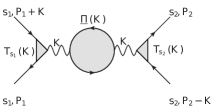
Figure 10: A diagram contributing to $\Gamma^{0}$.

III.6.5 Diffusive Fermi liquid theory

The full amplitudes $\Gamma^{0+1}\left(K\right)$, $\Gamma^{2}\left(K\right)$ and $\Gamma^{c}\left(K\right)$ contain, among others, diagrams describing multiple particle-hole (in the Cooper channel, particle-particle) scattering (see Appendix C). The very idea of dirty FL lies in replacing the dynamic part of these particle-hole (particle-particle) sections by their diffusive counterpart.Finkelstein (1990); Finkel’stein (2010) In particular, only the zeroth angular harmonic of the scattering amplitudes survives in the diffusive limit.

The scattering amplitude $\Gamma^{2}_{12}$ (as well as $\Gamma^{c}_{12}$) contains only particle-hole (respectively, particle-particle) sections consisting of modes from opposite surfaces of the topological insulator. Since we assume the disorder to be uncorrelated between the surfaces, these modes will not become diffusive and are hence not of interest for the present investigation. We therefore do not consider $\Gamma^{2}_{12}$ and $\Gamma^{c}_{12}$ any longer. As one can see from figures 6 - 8, the large angle scattering amplitudes $\Gamma^{2}_{11}$ and $\Gamma^{2}_{22}$ cannot be distinguished from the small angle scattering amplitudes $\Gamma^{0+1}_{11}$ and $\Gamma^{0+1}_{22}$, respectively. We incorporate the effect of $\Gamma^{2}_{11}$ and $\Gamma^{2}_{22}$ into the “singlet channel”, which has the following matrix structure in the surface space

$$\underline{\Gamma}^{\rho}=\left(\begin{array}[]{cc}\Gamma^{0+1-2}_{11}&\Gamma^{0+1}_{12}\\ \Gamma^{0+1}_{12}&\Gamma^{0+1-2}_{22}\end{array}\right).$$ (57)

Here we used

$$\Gamma^{0+1-2}=\Gamma^{0+1}-\Gamma^{2}.$$ (58)

The intrasurface Cooper channel interaction $\Gamma^{c}_{ss}$ will be also neglected. Its bare value is repulsive for the Coulomb interaction, so that the Cooper renormalization on ballistic scales $1/\tau\ll E\ll|\mu|$ renders it small on the UV scale of the diffusive theory (i.e., at the mean free path). Within the diffusive RG of a single 3D TI surface it quickly becomes of the order of $1/\sqrt{\sigma}$ and thus negligible (see Ref. Finkelstein, 1990 and supplementary material of Ref. Ostrovsky et al., 2010). Consequently we drop the Cooper channel amplitude and do not consider the superconductive instability in this work. For the opposite case of attraction in the Cooper channel Coulomb interaction suppresses the transition temperature $T_{c}$ .Finkel’stein (1987) The difference between Coulomb and short-range repulsive interaction was addressed in Ref. Burmistrov et al., 2012.

III.6.6 Bosonization of Fermi Liquid

The non-Abelian bosonization relies on the Dirac nature of the 2D electrons and on the associated non-Abelian anomaly. On the other hand, for $\alpha\sim 1$ the spectrum of the system gets strongly renormalized by interaction. An appropriate description in such a situation is the FL theory which is restricted to fermionic excitations close to the Fermi level. So, one can ask whether the result of non-Abelian bosonization remains applicable for $\alpha\sim 1$. The answer is yes, for the follwing reasons. All terms of the bosonized theory except for the $\mathbb{Z}_{2}$ theta term are determined by fermionic excitations close to the Fermi energy. Therefore, they equally hold for the FL if the coupling constants are appropriately redefined in terms of the corresponding FL parameters.

On the other hand, the $\mathbb{Z}_{2}$ theta term is a consequence of the chiral anomaly and thus the only term determined by energies far from $\mu$. However, it is well known that anomalies in quantum field theories are insensitive to interactions. Hence, the $\mathbb{Z}_{2}$ term in the diffusive NL$\sigma$M persists even for $\alpha\sim 1$. This follows also from the key property of the FL state: its spectrum is adiabatically connected to the free spectrum. This implies that topological implications remain unchanged. To summarize, the only difference between the NL$\sigma$M for the weakly interacting Fermi gas ($\alpha\ll 1$) and the FL ($\alpha\sim 1$) is the replacement of the interaction strength by the appropriate FL constant,

$$\underline{U}^{q}\rightarrow-\underline{\Gamma}^{\rho}$$

in Eq. (47).

III.6.7 Bare value of scattering amplitudes

According to the formal FL treatment (Appendix C.4), the singlet-channel interaction amplitude is given by

$$\underline{\nu}\underline{\Gamma}^{\rho}\underline{\nu}=-\underline{\nu}-\frac{\det\underline{\Pi}^{q}}{\Pi^{q}_{11}+\Pi^{q}_{22}+2\Pi^{q}_{12}}\left(\begin{array}[]{cc}1&-1\\ -1&1\end{array}\right),$$ (59)

where $(\underline{\nu})_{ss^{\prime}}=\nu_{s}\delta_{ss^{\prime}}$ and

$$\underline{\Pi}^{q}=-\underline{\nu}-\underline{\nu}\left(\begin{array}[]{cc}\Gamma^{1-2}_{11}&\Gamma^{1}_{12}\\ \Gamma^{1}_{12}&\Gamma^{1-2}_{22}\end{array}\right)\underline{\nu}.$$ (60)

Here $\Gamma^{1-2}=\Gamma^{1}-\Gamma^{2}$. The remarkably simple matrix structure of $\underline{\nu}+\underline{\nu}\underline{\Gamma}^{\rho}\underline{\nu}$ is actually due to the presence of the long-range Coulomb interaction. This fact will be explained by means of $\mathcal{F}$-invariance in section III.7.2. It has very important consequences for the RG flow in the diffusive regime, see Sec. IV.2.

III.6.8 Action of NL$\sigma$M

We are now in a position to present the full action of the diffusive interacting NL$\sigma$M for the problem under consideration:

$$S=\sum_{s}\left[S^{({\rm kin})}_{s}+iS^{(\theta)}_{s}\right]+S^{(\eta\,+\,{\rm int})}.$$ (61)

It contains the kinetic term

$$S^{({\rm kin})}_{s}=\frac{\sigma_{s}}{16}\int_{\textbf{{x}}}\text{tr}\left(\nabla Q_{s}\right)^{2}$$ (62)

and the ${\mathbb{Z}}_{2}$ theta term

$$S^{(\theta)}_{s}=\frac{1}{24\pi}\left.\Gamma_{s}\right|_{\tilde{O}_{s}\left(\textbf{{x}},w=1\right)=Q_{s}\left(\textbf{{x}}\right)=Q_{s}^{T}\left(\textbf{{x}}\right)}$$ (63)

for each of the surfaces, as well as the frequency and interaction terms,

$$S^{(\eta\,+\,{\rm int})} = -\pi T\left[\sum_{s}2z_{s}\text{tr}\hat{\eta}Q_{s}\right.$$ (64)

$$- \left.\sum_{ss^{\prime};n,\alpha}\text{tr}\left[J_{n}^{\alpha}Q_{s}\right]\Gamma_{ss^{\prime}}\text{tr}\left[J_{-n}^{\alpha}Q_{s^{\prime}}\right]\right].$$

Here we have introduced the notation

$$\Gamma_{ss^{\prime}}=\frac{8}{\pi}\lambda_{s}\Gamma^{\rho}_{ss^{\prime}}\lambda_{s^{\prime}}.$$ (65)

III.7 Inclusion of scalar and vector potentials into the NL$\sigma$M

In this subsection, we investigate consequences of the gauge invariance for the interacting NL$\sigma$M.

III.7.1 Electromagnetic gauge invariance

We include the scalar potential $\Phi_{s}$ and the vector potential $A_{\mu,s}$ for surface $s$ in the microscopic action (13) by means of covariant derivatives. This makes the action gauge-invariant, i.e., unchanged under local $\mathbf{U}(1)$-rotations of the fermionic fields $\psi$ and $\bar{\psi}$ accompanied by the corresponding gauge transformation of the potentials. Note that locality implies independent rotations on the top and bottom surfaces of the TI film.

The rotations of $\psi$-fields imply the following rotation of bispinors:

$$\eta_{s}\left(\textbf{{x}}\right)\rightarrow W_{s}\eta_{s}\left(\textbf{{x}}\right),$$ (66)

where

$$W_{s}=\left[e^{-i\hat{\chi}_{s}^{T}}\frac{1+\tau_{y}}{2}+e^{i\hat{\chi}_{s}}\frac{1-\tau_{y}}{2}\right]$$ (67)

and we use the following convention for hatted matrices: $\hat{a}\equiv\sum_{n,\alpha}a_{n}^{\alpha}I_{n}^{\alpha}$. Let us recall that the $\eta_{s}$ fields are considered as vectors in the Matsubara space. Upon introducing replica indices in the theory, the $\mathbf{U}(1)$ rotation angles and correspondingly the gauge potentials get replicated as well.

III.7.2 $\mathcal{F}$-algebra and $\mathcal{F}$-invariance

As a direct consequence of (66), $Q$-matrices transform under a gauge transformation $\chi_{s}$ in the following way:

$$Q_{s}\rightarrow W_{s}Q_{s}W_{s}^{T}.$$ (68)

Under such rotations, in the limit $N_{M}^{\prime},N_{M}\to\infty$, $N_{M}/N_{M}^{\prime}\to 0$, the frequency term acquires the correction Pruisken et al. (1999)

$$\delta_{\chi}\text{tr}\hat{\eta}Q_{s}=2\sum_{n,\alpha}\left[in\chi_{s,n}^{\alpha}\text{tr}J_{-n}^{\alpha}Q_{s}-n^{2}\chi_{s,n}^{\alpha}\chi_{s,-n}^{\alpha}\right],$$ (69)

while the factors entering the interaction term vary as follows:

$$\delta_{\chi}\text{tr}J_{n}^{\alpha}Q_{s}=-i2n\chi_{s,n}^{\alpha}.$$ (70)

As explained in Sec. III.1, the presence of the Coulomb interaction implies invariance of the fermionic action (13) under a simultaneous rotation in both surfaces by the same spatially constant (“global”) but time-dependent $\mathbf{U}(1)$-phase even without inclusion of gauge potentials (“$\mathcal{F}$-invariance”). This symmetry has to be preserved on NL$\sigma$M level, implying that

$$\left(\underline{z}+\underline{\Gamma}\right)\left(\begin{array}[]{c}1\\ 1\end{array}\right)=0.$$ (71)

Here $(\underline{z})_{ss^{\prime}}=z_{s}\delta_{ss^{\prime}}$. Since the intersurface interaction is symmetric, $\Gamma_{12}=\Gamma_{21}$, Eq. (71) yields

$$\underline{z}+\underline{\Gamma}=\text{const.}\times\left(\begin{array}[]{cc}1&-1\\ -1&1\end{array}\right).$$ (72)

This relation is consistent with Eq. (59). However, contrary to Eq. (59), the relation (72) is manifestly imposed by the symmetry (“$\mathcal{F}$-invariance”) of the action (61). It should therefore remain intact under RG flow.

III.7.3 Gauging the NL$\sigma$M and linear-response theory

Generally, the requirement of gauge invariance prescribes the correct coupling to the scalar and vector potentials in the action of the NL$\sigma$M, Eq. (61). In particular, in the kinetic term one has to replace $\partial_{\mu}Q_{s}\rightarrow D_{\mu,s}Q_{s}$ with the long derivative $D_{\mu}$ of the form

$$D_{\mu,s}Q_{s}\equiv\partial_{\mu}Q_{s}+\sum_{n,\alpha}iA^{\alpha}_{\mu,s,-n}\left[J_{n}^{\alpha}-\left(J_{n}^{\alpha}\right)^{T},Q_{s}\right].$$ (73)

For simplicity, the electron charge is absorbed into the vector potential here and in the following subsection.

As the theory is non-local in the imaginary time, the inclusion of the scalar potential is non-linear. The corresponding term that should be added to the NL$\sigma$M (61) reads

$$S^{\Phi} = -2\sum_{n\alpha,ss^{\prime}}{\Phi_{n,s}^{\alpha}}{\left(\underline{z}+\underline{\Gamma}\right)_{ss^{\prime}}}\text{tr}J_{n}^{\alpha}Q_{s}$$ (74)

$$+ \frac{1}{\pi T}\sum_{n\alpha,ss^{\prime}}{\Phi_{n,s}^{\alpha}}{\left(\underline{z}+\underline{\Gamma}\right)_{ss^{\prime}}}\Phi_{-n,s}^{\alpha}.$$

The inclusion of the scalar and vector potentials allow us to express the density-density correlation function and the conductivity in terms of the matrix fields $Q_{s}$ by means of the linear-response theory. In particular, a double differentiation of the partition function with respect to the scalar potential yields the density-density response,

$$\Pi^{\rm RPA}_{ss^{\prime}}\left(\omega_{n},\textbf{{q}}\right) = -\frac{2}{\pi}\left(z+\Gamma\right)_{ss^{\prime}}$$ (75)

$$+4T\sum_{s_{1},s_{2}}\left(z+\Gamma\right)_{ss_{1}}\left\langle\text{tr}J_{n}^{\alpha}Q_{s_{1}}\left(\textbf{{q}}\right)\right.\times$$

$$\times\left.\text{tr}J_{-n}^{\alpha}Q_{s_{2}}\left(-\textbf{{q}}\right)\right\rangle\left(z+\Gamma\right)_{s_{2}s^{\prime}}.$$

Here $\left\langle...\right\rangle$ denotes average with respect to the action (61). The superscript ^RPA emphasizes that the quantity appearing in the total density-density response includes RPA resummation. It is thus one-Coulomb-line-reducible and only its irreducible part corresponds to the polarization operator.

In the same spirit, we obtain the expression for the conductivity (in units of $e^{2}/h$) at a finite, positive frequency $\omega_{n}$:

$$\sigma^{\prime}_{ss^{\prime}}\left(\omega_{n}\right)=B^{(s)}_{1}\delta_{ss^{\prime}}+B^{(ss^{\prime})}_{2}.$$ (76)

Here we introduced two correlators:

$$B^{(s)}_{1}=\frac{\sigma_{s}}{8n}\left\langle\text{tr}\left[J_{n}^{\alpha}-\left(J_{n}^{\alpha}\right)^{T},Q_{s}\right]\left[J_{-n}^{\alpha}-\left(J_{-n}^{\alpha}\right)^{T},Q_{s}\right]\right\rangle$$ (77)

and

$$B^{(ss^{\prime})}_{2} = \frac{\sigma_{s}\sigma_{s^{\prime}}}{128n}\int_{\textbf{{x}}-\textbf{{x}}^{\prime}}\sum_{\mu=x,y}$$ (78)

$$\left\langle\text{tr}\left\{\left[J_{n}^{\alpha}-\left(J_{n}^{\alpha}\right)^{T},Q_{s}\right]\partial_{\mu}Q_{s}\right\}_{\textbf{{x}}}\times\right.$$

$$\times\left.\text{tr}\left\{\left[J_{-n}^{\alpha}-\left(J_{-n}^{\alpha}\right)^{T},Q_{s^{\prime}}\right]\partial_{\mu}Q_{s^{\prime}}\right\}_{\textbf{{x}}^{\prime}}\right\rangle.$$

Substituting the saddle-point value $Q_{s}=\Lambda$, we obtain the classical value $\sigma^{\prime}_{ss^{\prime}}\left(\omega_{n}\right)=\sigma_{s}\delta_{ss^{\prime}}$. Hence the dimensionless coupling constant of the NL$\sigma$M has been identified with the physical conductivity in units of $e^{2}/h$.

III.7.4 Gauging the theta term and anomalous quantum Hall effect

The local expression of the $\mathbb{Z}_{2}$ theta term, i.e, the WZW-term, Eq. (63), also allows of inclusion of gauge potentials. Polyakov and Wiegmann (1983); Vecchia et al. (1984); Faddeev (1976); Gerasimov (1993); Losev et al. (1995); Smilga (1996) However, the situation is more subtle here. Specifically, it turns out that the contribution of non-singular gauge potentials to the topological term $S^{(\theta)}$ vanishes. We explicitly show this in Appendix A.1.

The situation changes when the time-reversal symmetry is broken (at least, in some spatial domain at the surface) by a random or/and unform magnetic field. Subjected to a strong magnetic field, 3D TI surface states display the characteristic quantum Hall effect of Dirac electrons Brüne et al. (2011); Nomura et al. (2008) with quantized transverse conductance

$$\sigma_{xy}=g\left(n\pm\frac{1}{2}\right)\frac{e^{2}}{h},\;n\in\mathbb{Z},$$ (79)

where $g$ is the degeneracy of Dirac electrons, e.g., $g=2$ for two 3D TI surfaces. It is intimately linked to the topological magnetoelectric effect.Qi et al. (2008, 2009); Essin et al. (2009); Pesin and MacDonald (2012) Theoretically, the anomalous quantum Hall effect was explained and discussed in a previous work by three of the authors. Ostrovsky et al. (2008) We will explain in the following how to understand it in the framework of the linear response theory within the NL$\sigma$M. As it turns out, the crucial point is that gauge potentials drop from $S^{(\theta)}$.

We first briefly recall the NL$\sigma$M field theory describing the ordinary integer QHE (i.e., for electrons with quadratic dispersion). It contains Pruisken’s theta term, Pruisken (1990) which assumes the following form upon inclusion of the vector potential: Pruisken et al. (1999)

$$S^{\text{QHE}}= \frac{\vartheta}{16\pi}\int_{\textbf{{x}}}\epsilon_{\mu\nu}\text{tr}Q_{U}\partial_{\mu}Q_{U}\partial_{\nu}Q_{U}$$ (80a)

$$+\frac{i\vartheta}{4\pi}\int_{\textbf{{x}}}\epsilon_{\mu\nu}\text{tr}\partial_{\mu}\hat{A}_{\nu}Q_{U}$$ (80b)

$$+\frac{\vartheta}{4\pi}\int_{\textbf{{x}}}\epsilon_{\mu\nu}\sum_{n,\alpha}nA_{\mu,n}^{\alpha}A_{\nu,-n}^{\alpha}.$$ (80c)

Here $Q_{U}=U^{-1}\Lambda U$ with $U\in\mathbf{U}\left(2N_{M}\times N_{R}\right)$, $\epsilon_{\mu\nu}=-\epsilon_{\nu\mu}$ is the 2D antisymmetric symbol ($\epsilon_{xy}\stackrel{{\scriptstyle\text{def.}}}{{=}}1$), and $\vartheta$ is the theta angle of the Pruisken’s NL$\sigma$M. We emphasize, that the last two terms (Eqs. (80b) and (80c)) determine the effective electromagnetic response and thus prescribe the relation between the physical observable $\sigma_{xy}$ (in units of $e^{2}/h$) and the theta angle $\vartheta$. In particular, $\vartheta/2\pi$ is identified as the bare value of the Hall conductance.Pruisken and Burmistrov (2005)

Let us now turn to a single Dirac surface state. As has been discussed above, all gauge potentials drop from $S^{(\theta)}$. Let us first add a random magnetic field (keeping zero average magnetic field) to the gauged NL$\sigma$M. This implies a breakdown of the symmetry:

$$\mathcal{M}\rightarrow\frac{\mathbf{U}\left(2N_{M}N_{R}\right)}{\mathbf{U}\left(N_{M}N_{R}\right)\times\mathbf{U}\left(N_{M}N_{R}\right)}.$$ (81)

The $\mathbb{Z}_{2}$ theta term becomes the Pruisken’s theta term Bocquet et al. (2000) (recall $\theta=\pi\,\text{mod}\,2\pi$)

$$S^{(\theta)}_{U}=\frac{\theta}{16\pi}\int_{\textbf{{x}}}\epsilon_{\mu\nu}\text{tr}Q_{U}\partial_{\mu}Q_{U}\partial_{\nu}Q_{U}.\\$$ (82)

We emphasize that together with the gauged kinetic term $S^{(\theta)}_{U}$ is the complete gauged theory, no extra terms of the type (80b) and (80c) appear. Being topological, the Pruisken’s theta term is invariant under smooth $\mathbf{U}\left(1\right)$ rotations. Recall that exactly the terms (80b) and (80c) provided a link between $\vartheta$ and $\sigma_{xy}$ in the conventional (non-Dirac) QHE setting. Their absence in Eq. (82) is thus physically very natural: without a net magnetic field the Hall conductivity is zero.

We consider now the case when the average magnetic field is non-zero. The action of the NL$\sigma$M describing a Dirac fermion is then given by a sum of Eqs. (80) and (82). The renormalization of the action of the NL$\sigma$M is governed by the full theta angle $\vartheta+\theta$. On the other hand, only $\vartheta$ is related with the bare value of $\sigma_{xy}$. Then standard arguments for the quantization of the Hall conductivity Pruisken and Burmistrov (2007) leads to the result (79) for the anomalous QHE.

IV One-loop RG

In the preceding section we have derived the diffusive NL$\sigma$M, Eqs. (61). We will now investigate its behavior under renormalization. This will allow us, in particular, to deduce the scale dependence of the conductivity. The most important steps of the calculation are presented in the main text; further details can be found in Appendix D.

We calculate the renormalization of the NL$\sigma$M parameters within the linear-response formalism (rather than the background-field method). This is favorable since it implies a more direct physical interpretation of the NL$\sigma$M coupling constants. Furthermore, this way one can in principle treat simultaneously different infrared regulators, such as temperature or frequency. However, for the sake of clarity of presentation we restrict ourselves to a purely field-theoretical regularization scheme and add a mass term to the action

$$S_{L}=-\sum_{s=1,2}\frac{\sigma_{s}L^{-2}}{8}\int_{\textbf{{x}}}\text{tr}\Lambda Q_{s}.$$ (83)

The connection between the running length scale $L$ and the physical regulators temperature or frequency was analyzed in Ref. [Baranov et al., 1999]. Roughly speaking, in the presence of a single infrared scale $E$, e.g. when calculating DC conductance at finite temperature and assuming an infinite sample, one can replace $L$ by $L_{E}$ in the results.

We will calculate all UV-divergent contributions in the dimensional regularization scheme. This allows us to preserve the local $\text{O}\left(2_{\tau}\times N_{M}\times N_{R}\right)\times\text{O}\left(2_{\tau}\times N_{M}\times N_{R}\right)$-symmetry of the $Q$-matrix (42) and to ensure the renormalizability of the theory.

IV.1 Diffusive propagators

We employ the exponential parametrization of the matrix fields $Q_{s}=\Lambda\exp W_{s}$. The antisymmetric fields

$$W_{s}=\left(\begin{array}[]{cc}0&q_{s}\\ -q_{s}^{T}&0\end{array}\right)$$

anticommute with $\Lambda$. Further, we define a set of real matrices in the particle-hole space: $\tilde{\tau}_{\mu}\equiv 2^{-1/2}\left(\mathbf{1},\tau_{x},i\tau_{y},\tau_{z}\right)$. This allows us to introduce the fields $q^{(\mu)}\equiv\text{tr}^{\tau}q\tilde{\tau}_{\mu}^{T}$, where $\text{tr}^{\tau}$ is the trace in the particle-hole space only. With these definitions at hand, we expand the action, Eqs. (61) and (83), to quadratic order in $q^{(\mu)}$ and obtain the NL$\sigma$M propagators that describe the diffusive motion in the particle-hole (diffusons) and particle-particle (cooperons) channels.

The fields $q^{(1)}$ and $q^{(3)}$ describe cooperons. Their propagator is unaffected by interaction (since we have discarded the interaction in the Cooper channel),

$$\left\langle\left[q_{s}^{(\mu)}(\textbf{{p}})\right]_{m_{1}m_{2}}^{\alpha_{1}\alpha_{2}}\left[q_{s^{\prime}}^{(\nu)}(-\textbf{{p}})\right]_{n_{1}n_{2}}^{\beta_{1}\beta_{2}}\right\rangle=\frac{4}{\sigma_{s}}D_{s}\left(\omega_{n_{12}},\textbf{{p}}\right)\delta_{ss^{\prime}}$$

$$\hfill\times\delta_{\mu\nu}\delta_{n_{1}m_{1}}\delta_{n_{2}m_{2}}\delta_{\alpha_{1}\beta_{1}}\delta_{\alpha_{2}\beta_{2}}\bigl{(}\delta_{\mu 1}+\delta_{\mu 3}\bigr{)},\hskip 8.5359pt{}\,$$ (84)

where

$$\bigl{[}D_{s}\left(\omega_{n_{12}},\textbf{{p}}\right)\bigr{]}^{-1}=\textbf{{p}}^{2}+L^{-2}+\frac{4z_{s}}{\sigma_{s}}\omega_{n_{12}}.$$ (85)

The Matsubara indices $n_{1}$, $m_{1}$ are non-negative, while the indices $n_{2}$, $m_{2}$ are negative; we have also defined $n_{12}\equiv n_{1}-n_{2}>0$ and $m_{12}\equiv m_{1}-m_{2}>0$.

Next, we consider the diffusons $q^{(0)}$ and $q^{(2)}$. Their Green’s function, written as a matrix in surface space, is

$$\left\langle\left[q^{(\mu)}_{s}(\textbf{{p}})\right]_{m_{1}m_{2}}^{\alpha_{1}\alpha_{2}}\left[q^{(\nu)}_{s^{\prime}}(-\textbf{{p}})\right]_{n_{1}n_{2}}^{\beta_{1}\beta_{2}}\right\rangle=\displaystyle\frac{4}{\sigma_{s}}D_{s}\left(\omega_{n_{12}},\textbf{{p}}\right)\delta_{\mu\nu}$$

$$\times\delta_{n_{12},m_{12}}\delta_{\alpha_{1}\beta_{1}}\delta_{\alpha_{2}\beta_{2}}\bigl{(}\delta_{\mu 0}+\delta_{\mu 2}\bigr{)}$$

$$\times\left[\delta_{n_{1}m_{1}}\delta_{ss^{\prime}}-\displaystyle\frac{8\pi T}{\sigma_{s^{\prime}}}\delta^{\alpha_{1}\alpha_{2}}\left(\underline{\Gamma D^{c}}\left(\omega_{n_{12}},\textbf{{p}}\right)\right)_{ss^{\prime}}\right].$$ (86)

Here we have introduced

$$\bigl{[}D^{c}\left(\omega_{n_{12}},\textbf{{p}}\right)\bigr{]}^{-1}_{ss^{\prime}}=D_{s}^{-1}\left(\omega_{n_{12}},\textbf{{p}}\right)\delta_{ss^{\prime}}+\frac{4\omega_{n_{12}}}{\sigma_{s}}\Gamma_{ss^{\prime}}.$$ (87)

IV.2 RG invariants

The bare action contains, aside from the mass $L^{-1}$, seven running coupling constants: $\sigma_{1}$, $\sigma_{2}$, $z_{1}$, $z_{2}$, $\Gamma_{11}$, $\Gamma_{22}$ and $\Gamma_{12}$. We are now going to show that three linear combinations of them are conserved under RG. To this end we evaluate the density-density response (75) at the tree level:

$$\underline{\Pi}^{\rm RPA}\left(\omega,\textbf{{p}}\right)=-\frac{2}{\pi}\left[\underline{z}+\underline{\Gamma}\right]\bigl{(}1-4\omega\underline{\sigma^{-1}D^{c}}\left(\omega,\textbf{{p}}\right)\left[\underline{z}+\underline{\Gamma}\right]\bigr{)}$$ (88)

where $(\underline{\sigma})_{ss^{\prime}}=\sigma_{s}\delta_{ss^{\prime}}$. There is no need for infrared regularization here and we therefore omit the mass term (83).

On the other hand, the density-density response function can be obtained from the fermionic formulation of the theory, see Appendix C.5:

$$\underline{\Pi}^{\rm RPA}=\left[\underline{\Pi}^{q}-\underline{\nu\Gamma}^{0}\underline{\nu}\right]\left(1+\omega\underline{\Delta}^{\Gamma}\left(\omega,\textbf{{p}}\right)\left[\underline{\Pi}^{q}-\underline{\nu\Gamma}^{0}\underline{\nu}\right]\right),$$ (89)

where

$$\Delta^{\Gamma}\left(\omega,\textbf{{p}}\right)=\left[\underline{\nu D}\textbf{{p}}^{2}+\omega\left(\underline{\nu}+\underline{\nu}\underline{\Gamma}^{\rho,q}\underline{\nu}\right)\right]^{-1}.$$ (90)

The equality of Eqs. (88) and (89) relates two functions of momentum and frequency. In the static limit, we find the following constraint connecting the NL$\sigma$M coupling constants with physical FL parameters:

$$\frac{2}{\pi}\left(\underline{z}+\underline{\Gamma}\right)=-\underline{\Pi^{q}}+\underline{\nu}\underline{\Gamma^{0}}\underline{\nu}.$$ (91)

Next, from comparison of momentum dependence in Eqs. (88) and (89), we find the Einstein relation: $\sigma_{s}=2\pi\nu_{s}D_{s}$. Accordingly, $\sigma$ measures the conductance in units of $e^{2}/h$, consistently with what has been found in Secs. III.2 and III.7.3.

In view of gauge invariance (Sec. III.6.4), the static polarization operator entering Eq. (91) is nothing but the compressibility

$$\Pi^{ss^{\prime},q}=-\frac{\partial N_{s}}{\partial\mu_{s^{\prime}}}.$$

Its value is not renormalized because it can be expressed as a derivative of a physical observable with respect to the chemical potentials. On ballistic scales the chemical potential enters logarithmically divergent corrections only as the UV cutoff of the integrals. In the diffusive regime, the UV cutoff is provided by the scattering rates $\tau^{-1}_{s}\ll|\mu_{s}|$. Therefore, diffusive contributions to the derivative with respect to the chemical potential vanish.Finkelstein (1990) Since $\underline{\nu}\underline{\Gamma}^{0}\underline{\nu}$ only depends on $\underline{\Pi}^{q}$ (see Appendix C.4) it is not renormalized as well. Therefore, the right-hand side of (91) is not renormalized and hence neither is its left-hand-side, i.e., $\underline{z}+\underline{\Gamma}$. This matrix constraint yields three RG invariants: $z_{1}+\Gamma_{11}$, $z_{2}+\Gamma_{22}$, and $\Gamma_{12}$. Thus, only four out of seven NL$\sigma$M parameters are independent running coupling constants. We emphasize that, in contrast to Eq. (72), this reasoning is valid also in the absence of long-range interaction.

Finally, let us evaluate Eq. (91) on the bare level. Expressing the static polarization operator as $\underline{\Pi}^{q}=-\underline{\nu}-\underline{\nu}\underline{\Gamma^{1-2}}\underline{\nu}$ and using the definition of $z_{s}$ in Sec. III.5.1 one can find the following relations for the bare values

$$\frac{4\lambda_{s}}{\pi}\equiv\frac{2}{\pi}z_{s}=\nu_{s}.$$ (92)

Equivalently, the same relationship between $\lambda_{s}$ and $\nu_{s}$ can be obtained by comparing the bare definition of $\underline{\Gamma}$ [Eq. (65)] with the right hand side of (91). The relation (92) has been foreseen earlier on the basis of SCBA, see Eq. (40). In conclusion, the SCBA and the density response independently show that the UV cutoff scale for the bosonization is automatically set by the chemical potential (which is also very natural from the physical point of view).

IV.3 Renormalization of conductivities

IV.3.1 Correlator $B_{1}$

We will first analyze the correlator $B^{(s)}_{1}$, Eq. (77). The one-loop correction is determined by the expansion to second order in $q^{(\mu)}$. The tensor structure in particle-hole space implies that the diffuson contribution ($\mu=0,2$) vanishes. The classical value together with the cooperon contribution ($\mu=1,3$) is

$$B^{(s)}_{1}=\sigma_{s}+2\int_{\textbf{{p}}}D_{s}(\omega_{n},\textbf{{p}}).$$ (93)

We evaluate this term in the announced regularization scheme:

$$B^{(s)}_{1} = \sigma_{s}+2\text{I}^{(2+\epsilon)}_{1}$$ (94)

$$= \sigma_{s}+\frac{1}{2\pi}\left[-\frac{2}{\epsilon}+2\ln{L}/{l}+\text{const.}\right].$$ (95)

For dimensional reasons we have introduced the reference length scale $l$, which for the present diffusive problem is set by the mean free path $l=\max_{s=1,2}l_{s}$. We have further evaluated the following standard dimensionless integral

$$\text{I}^{(D)}_{1} \equiv l^{D-2}\int\frac{d^{D}p}{\left(2\pi\right)^{D}}\frac{1}{\textbf{{p}}^{2}+L^{-2}}$$

$$= \frac{\left(\frac{l^{2}}{L^{2}}\right)^{\frac{D}{2}-1}}{\left(4\pi\right)^{\frac{D}{2}}}\Gamma\left(1-\frac{D}{2}\right)$$

$$\stackrel{{\scriptstyle D=2+\epsilon}}{{=}} \frac{1}{4\pi}\left[-\frac{2}{\epsilon}+2\ln{L}/{l}+\ln 4\pi-\bm{\gamma}+\mathcal{O}\left(\epsilon\right)\right],$$

where $\bm{\gamma}\approx 0,577$ is the Euler-Mascheroni constant.

The logarithmic term in Eq. (95) is nothing but the well-known weak-antilocalization effect.Hikami et al. (1980)

IV.3.2 Correlator $B_{2}$

Next we turn our attention to $B^{(ss^{\prime})}_{2}$, Eq. (78). Because of the presence of gradients it does not contribute neither at classical nor at tree level. Furthermore, due to the absence of the Cooper channel and the uncorrelated disorder on the top and bottom surfaces, there are no quantum corrections to the transconductance $\sigma_{12}$. The correlator $B^{(ss^{\prime})}_{2}$ can be recast into the form (see Appendix D)

$$B_{2}^{(ss^{\prime})} = \frac{16\delta_{ss^{\prime}}}{n\sigma_{s}}\int_{\textbf{{p}}}\textbf{{p}}^{2}\sum_{\omega_{m}>0}\omega_{m}$$ (96)

$$\times\Bigl{[}\left(\underline{D\Gamma D^{c}}\right)_{ss}\left(\omega_{m},{\textbf{{p}}}\right)D_{s}\left(\omega_{m+n},{\textbf{{p}}}\right)$$

$$-\left(\underline{D\Gamma D^{c}}\right)_{ss}\left(\omega_{m+n},{\textbf{{p}}}\right)D_{s}\left(\omega_{m+2n},{\textbf{{p}}}\right)\Bigr{]}.$$

For its evaluation it is instructive to separate contributions stemming from intrasurface interaction $\Gamma_{ss}$ and intersurface interaction $\Gamma_{12}$. This leads to

$$B_{2}^{ss^{\prime}} = -4\delta_{ss^{\prime}}\left(\underbrace{1-\frac{1+\gamma_{ss}}{\gamma_{ss}}\ln\left(1+\gamma_{ss}\right)}_{\text{single surface}}\right.$$ (97)

$$+ \left.\underbrace{\left(1+\gamma_{ss}\right)\left(\frac{\ln\left(1+\gamma_{ss}\right)}{\gamma_{ss}}-\frac{\ln\left(1+\tilde{\gamma}_{ss}\right)}{\tilde{\gamma}_{ss}}\right)}_{\text{intersurface interaction}}\right)I_{2}^{(2+\epsilon)}$$

$$= -\frac{\delta_{ss^{\prime}}}{\pi}\left(1-\frac{1+\gamma_{ss}}{\tilde{\gamma}_{ss}}\ln\left(1+\tilde{\gamma}_{ss}\right)\right)\times$$

$$\times\left[-\frac{2}{\epsilon}+2\ln L/l+\text{const}\right].$$

We have introduced $\gamma_{ss}=\Gamma_{ss}/z_{s}$, $\tilde{\gamma}_{11}=\gamma_{11}+(\sigma_{1}/\sigma_{2})(1+\gamma_{11})$ and $\tilde{\gamma}_{22}=\gamma_{22}+(\sigma_{2}/\sigma_{1})(1+\gamma_{22})$. Note that in the limit of $z_{2}+\Gamma_{22}=0$ [which corresponds to $\Gamma_{12}=0$ in view of (72)] we recover the well-known conductivity corrections to $\sigma_{11}$ for a single surface (see also Sec. V.2.1). Further, in Eq. (97) we have evaluated the second standard diverging integral

$$\text{I}^{(D)}_{2} \equiv l^{D-2}\int\frac{d^{D}p}{\left(2\pi\right)^{D}}\frac{\textbf{{p}}^{2}}{\left(\textbf{{p}}^{2}+L^{-2}\right)^{2}}$$

$$= \frac{\left(\frac{l^{2}}{L^{2}}\right)^{\frac{D}{2}-1}}{\left(4\pi\right)^{\frac{D}{2}}}\frac{D}{2}\Gamma\left(1-\frac{D}{2}\right)$$

$$\stackrel{{\scriptstyle D=2+\epsilon}}{{=}} \frac{1}{4\pi}\left[-\frac{2}{\epsilon}+2\ln{L}/{l}+\ln 4\pi-1-\bm{\gamma}+\mathcal{O}\left(\epsilon\right)\right].$$

IV.4 Renormalization of the interaction amplitudes

The renormalization of the interaction amplitudes, or equivalently, of Finkelstein parameters $z_{s}$, is intimately linked to the renormalization of the specific heat. Castellani and Di Castro (1986) This is because the scale (e.g., temperature) dependence of the total thermodynamic potential $\Omega$ is governed by the scale dependence of $z_{s}$. In the present case of coupled surfaces we can only extract the correction to the sum $z_{1}+z_{2}$ from the (one-loop) correction to the total thermodynamic potential: Baranov et al. (1999)

$$z^{\prime}_{1}+z^{\prime}_{2}=\frac{1}{2\pi\text{tr}\eta\Lambda}\frac{\partial}{\partial T}\frac{\Omega}{T}.$$ (98)

At the classical level Eq. (98) yields the relation $z^{\prime}_{1}+z^{\prime}_{2}=z_{1}+z_{2}$. Evaluating the quantum corrections in Eq. (98), we find

$$\left(z^{\prime}_{1}+z^{\prime}_{2}\right)=\left(z_{1}+z_{2}\right)+2\sum_{s=1,2}\Gamma_{ss}\int_{\textbf{{p}}}D_{s}\left(0,\textbf{{p}}\right).$$ (99)

As the correction is a sum of contributions from the two opposite surfaces, it is natural to assume that the parameters $z_{s}$ are renormalized $separately$ (and without intersurface interaction effects):

$$z_{s}^{\prime} = z_{s}+2\Gamma_{ss}\int_{\textbf{{p}}}D_{s}\left(0,\textbf{{p}}\right)$$ (100)

$$= z_{s}+2\frac{\Gamma_{ss}}{\sigma_{s}}\text{I}^{(2+\epsilon)}_{1}$$

$$= z_{s}+\frac{1}{2\pi}\frac{\Gamma_{ss}}{\sigma_{s}}\left[-\frac{2}{\epsilon}+2\ln L/l+\text{const}\right].$$

We have directly proven this assumption of separate $z_{s}$ renormalization by the background field method.

IV.5 The one-loop RG equations

Applying the minimal subtraction scheme to Eqs. (95), (97) and (100), we derive the one-loop perturbative RG equations:

$$\rule{0.0pt}{12.91663pt}\rule[-8.61108pt]{0.0pt}{0.0pt}\frac{d\sigma_{1}}{dy} =-\frac{2}{\pi}F\left(\gamma_{11},\frac{\sigma_{1}}{\sigma_{2}}\right),$$ (101a)

$$\rule{0.0pt}{12.91663pt}\rule[-8.61108pt]{0.0pt}{0.0pt}\frac{d\sigma_{2}}{dy} =-\frac{2}{\pi}F\left(\gamma_{22},\frac{\sigma_{2}}{\sigma_{1}}\right),$$ (101b)

$$\rule{0.0pt}{12.91663pt}\rule[-8.61108pt]{0.0pt}{0.0pt}\frac{d\gamma_{11}}{dy} =-\frac{\gamma_{11}\left(1+\gamma_{11}\right)}{\pi\sigma_{1}},$$ (101c)

$$\rule{0.0pt}{12.91663pt}\rule[-8.61108pt]{0.0pt}{0.0pt}\frac{d\gamma_{22}}{dy} =-\frac{\gamma_{22}\left(1+\gamma_{22}\right)}{\pi\sigma_{2}},$$ (101d)

where $y=\ln L/l$, $\gamma_{ss}=\Gamma_{ss}/z_{s}$, $l=\max_{s=1,2}l_{s}$ and

$$F\left(\gamma,x\right)=\frac{1}{2}-\frac{1+\gamma}{x\left[1+\gamma\left(1+\frac{1}{x}\right)\right]}\text{ln}\left[\left(1+x\right)\left(1+\gamma\right)\right].$$ (102)

We recall that $\Gamma_{12}$, $z_{1}+\Gamma_{11}$ and $z_{2}+\Gamma_{22}$ are not renormalized. We mention that the mass $L^{-1}$ acquires a quantum correction Baranov et al. (1999) but it does not affect the one-loop renormalization of the other parameters $\sigma_{s}$, $z_{s}$ and $\Gamma_{ss^{\prime}}$.

For an alternative presentation of the RG equations (101) we introduce the total conductivity $\sigma=\sigma_{1}+\sigma_{2}$ and the ratio of the conductivities of the two surfaces $t=\sigma_{1}/\sigma_{2}$. In terms of these parameters the RG equations take the following form:

$$\rule{0.0pt}{12.91663pt}\rule[-8.61108pt]{0.0pt}{0.0pt}\frac{d\sigma}{dy} =-\frac{2}{\pi}\left\{1-\frac{1}{t}\frac{1+\gamma_{11}}{1+\gamma_{11}\left(1+\frac{1}{t}\right)}\text{ln}\left[\left(1+{t}\right)\left(1+\gamma_{11}\right)\right]-{t}\frac{1+\gamma_{22}}{1+\gamma_{22}\left(1+{t}\right)}\text{ln}\left[\left(1+\frac{1}{t}\right)\left(1+\gamma_{22}\right)\right]\right\},$$ (103a)

$$\rule{0.0pt}{12.91663pt}\rule[-8.61108pt]{0.0pt}{0.0pt}\frac{dt}{dy} =-\frac{2}{\pi}\frac{1+t}{\sigma}\left\{\frac{1-t}{2}-\frac{1}{t}\frac{1+\gamma_{11}}{1+\gamma_{11}\left(1+\frac{1}{t}\right)}\text{ln}\left[\left(1+{t}\right)\left(1+\gamma_{11}\right)\right]+{t^{2}}\frac{1+\gamma_{22}}{1+\gamma_{22}\left(1+{t}\right)}\text{ln}\left[\left(1+\frac{1}{t}\right)\left(1+\gamma_{22}\right)\right]\right\},$$ (103b)

$$\rule{0.0pt}{12.91663pt}\rule[-8.61108pt]{0.0pt}{0.0pt}\frac{d\gamma_{11}}{dy} =-\left(1+\frac{1}{t}\right)\frac{\gamma_{11}\left(1+\gamma_{11}\right)}{\pi\sigma},$$ (103c)

$$\rule{0.0pt}{12.91663pt}\rule[-8.61108pt]{0.0pt}{0.0pt}\frac{d\gamma_{22}}{dy} =-\left(1+t\right)\frac{\gamma_{22}\left(1+\gamma_{22}\right)}{\pi\sigma}.$$ (103d)

V Analysis of the RG equations

It is worthwhile to remind the reader that the RG equations (101) describe the quantum corrections to conductivity due to the interplay of two distinct effects. First, they contain weak-antilocalization corrections (WAL) $\delta\sigma^{WAL}_{s}=(1/\pi)\ln L/l$ due to quantum interference in a disordered system with the strong spin-orbit coupling. Second, these are interaction-induced contributions of Altshuler-Aronov (AA) type, including effects of both, long-range and short-range interactions. The result (101) was obtained perturbatively to leading order in $1/\sigma_{s}\ll 1$ but it is exact in the singlet interaction amplitudes. While these equations describe the experimentally most relevant case of Coulomb interaction, in Appendix F we also present the RG equations for the case of short-range interaction.

Equations (101) which determine the flow of the coupling constants $\sigma_{1},\sigma_{2},\gamma_{11}$ and $\gamma_{22}$ imply a rich phase diagram in the four-dimensional parameter space. Before discussing the general four-dimensional RG flow we highlight the simpler case of two equal surfaces.

V.1 Two equal surfaces

Equal surfaces are defined by $\sigma_{1}=\sigma_{2}=\sigma/2$, $\gamma_{11}=\gamma_{22}=\gamma$ and, because of Eq. (72), $\gamma_{12}=-1-\gamma$. It can be checked that the plane of identical surfaces is an attractive fixed plane of the four dimensional RG-flow (see Appendix E). The RG equations for the two coupling constants $\sigma$ and $\gamma$ are

$$\rule{0.0pt}{12.91663pt}\rule[-8.61108pt]{0.0pt}{0.0pt}\frac{d\sigma}{dy} =-\frac{2}{\pi}\left[1-\frac{2+2\gamma}{1+2\gamma}\text{ln}\left(2+2\gamma\right)\right],$$ (104a)

$$\rule{0.0pt}{12.91663pt}\rule[-8.61108pt]{0.0pt}{0.0pt}\frac{d\gamma}{dy} =-\frac{2\gamma\left(1+\gamma\right)}{\pi\sigma}.$$ (104b)

Experimentally, the case of equal surfaces is realized if both surfaces are characterized by the same mean free path and the same carrier density and, furthermore, if the dielectric environment of the probe is symmetric ($\epsilon_{1}=\epsilon_{3}$).

V.1.1 Flow Diagram within the fixed plane

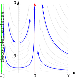
Figure 11: RG flow for equal surfaces in the parameter space $\sigma$ (total conductivity) and $\gamma$ (intra-surface interaction strength). Here and in all following RG diagrams, arrows indicate the flow towards the infrared.

The RG flow within the $\sigma$–$\gamma$ plane is depicted in Fig. 11. The green vertical fixed line at $\gamma=-1$ corresponds to the case of two decoupled surfaces (recall $\gamma_{12}=-1-\gamma$), and reproduces the result of Ref. Ostrovsky et al., 2010 for a single surface of 3D TI. In this limit the total correction to the conductivity is negative and obeys the universal law

$$\delta\sigma_{\gamma=-1}=2\times\frac{2}{\pi}\left(\underbrace{1/2}_{\rm WAL}-\underbrace{1}_{\rm AA}\right)\ln L/l=-\frac{2}{\pi}\ln L/l.$$ (105)

The line of decoupled surfaces is repulsive, as can be seen from Eq. (104b). Flowing towards the infrared, the conductivity first decreases before turning up again while the system approaches the second fixed line at $\gamma=0$. Note that on this line $\gamma_{12}=-1$: the intrasurface interaction has died out, but the intersurface interaction is maximal. Here the conductivity correction is positive indicating the flow into a metallic state:

$$\delta\sigma_{\gamma=0}=2\times\frac{2}{\pi}\left(\underbrace{1/2}_{\rm WAL}-\underbrace{\left[1-\ln 2\right]}_{\rm interaction}\right)\ln L/l.$$ (106)

The flow on this fixed line is towards the perfect-metal point

$$\left(1/\sigma^{*},t^{*},\gamma_{11}^{*},\gamma_{22}^{*}\right)=\left(0,1,0,0\right),$$

As discussed below, see Sec. V.2.2, this is the only attractive fixed point even in the case of the general four dimensional RG flow. On the $\gamma=0$ fixed line the intersurface interaction reduces the strength of the WAL effect but it is not strong enough to reverse the behavior. The region $\gamma>0$ corresponds to attractive interaction in the singlet channel and is shown on the flow diagram for the sake of completeness.

V.1.2 Typical bare values and crossover scale

Typically, before renormalization the intersurface interaction $\gamma_{12}$ is weaker than or equal to the intrasurface interaction $\gamma$. This implies that its bare value $\gamma_{0}$ takes values in the range between $\gamma_{0}=-1$ (decoupled surfaces, i.e. $\gamma_{12,0}=0$) and $\gamma_{0}=-1/2=\gamma_{12,0}$. For small $\alpha$ we can approximate $\gamma_{0}$ by its RPA value:

$$\gamma_{0}=-\frac{1}{2}-\frac{1}{2}\frac{\kappa d}{1+\kappa d}.$$ (107)

Here $d$ is the system thickness and $\kappa=2\pi\frac{e^{2}}{\epsilon_{2}}\nu$ the inverse single surface screening length obtained for the general symmetric situation: $\epsilon_{1}=\epsilon_{3}\neq\epsilon_{2}$, see Appendix B. Note that at $\kappa d=0$ the conductivity corrections due to WAL and AA exactly compensate each other:

$$\delta\sigma_{\gamma=-1/2}=\frac{2}{\pi}\left(2\times\underbrace{1/2}_{\rm WAL}-\underbrace{1}_{\rm AA}\right)\ln L/l=0,$$

as can also be seen in Fig. 11.

Typically $\kappa d>0$ or, as already explained on general grounds, $-1<\gamma_{0}<-1/2$. Then the most drastic consequence of intersurface interaction is the non-monotonic temperature (or length) dependence: the conductivity first decreases with lowering $T$ but eventually the sign of $d\sigma/dT$ changes and the system is ultimately driven into the metallic phase. It is natural to ask for the temperature scale, which is associated with this sign change. The scale $y_{*}$ at which the conductivity reaches its minimum can be extracted from Eqs. (104) and is expressed by the integral

$$y_{*}=-\frac{\pi\sigma_{0}}{2}\int_{\gamma_{0}}^{\gamma_{*}}\frac{d\gamma^{\prime}}{\gamma^{\prime}}\frac{1+\gamma_{0}}{(1+\gamma^{\prime})^{2}}\left[\frac{\gamma^{\prime}}{\gamma_{0}}\right]^{1-2\ln 2}e^{2\left[f\left(\gamma^{\prime}\right)-f\left(\gamma_{0}\right)\right]},$$ (108)

where $f\left(x\right)=\text{Li}_{2}\left(-x\right)-\text{Li}_{2}\left(-\left(1+2x\right)\right)$, Li₂ is the dilogarithm, and $\gamma_{*}=-1/2$.

Numerical integration of (108) yields the crossover length scale or temperature $y_{*}=\ln L_{*}/l=1/2\ln T_{0}/T_{*}$. Its dependence on the bare values $\sigma_{0}$ and $\gamma_{0}$ is plotted in Fig. 12. Using Eq. (107) one can also investigate the dependence of $y_{*}$ on $\kappa d$ instead of $\gamma_{0}$ (see inset in Fig.12).

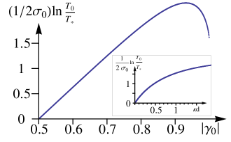
Figure 12: Temperature scale associated with the minimum of $\sigma$ as a function of the bare values $\sigma_{0}$ and $\gamma_{0}$. Inset: the same quantity as a function of $\sigma_{0}$ and $\kappa d$.

V.1.3 Role of topology: Dirac electrons vs. electrons with quadratic dispersion in the presence of spin-orbit interaction

The perturbative RG equations (101) and (104) are valid for $\sigma\gg 1$. Instanton effects are suppressed by $\exp(-2\pi\sigma)$ in this region and we therefore neglected them. As has been discussed in Sec. III.5.2, in the diffusive NL$\sigma$M of Dirac electrons, the $\mathbb{Z}_{2}$ theta term reflects the topological protection from Anderson localization. This term is absent in the case of non-topological symplectic metals (NTSM) such as electrons with quadratic dispersion subjected to strong spin-orbit coupling. The presence (respectively, absence) of the topological term results in the opposite signs of the instanton contribution in the two cases. However, as instantons are suppressed, our perturbative result is equally applicable to the surfaces of a 3D TI and, for example, to a double-quantum-well structure in a material with strong spin-orbit coupling. Here we discuss non-perturbative differences between the two problems.

Let us start from the case of decoupled surfaces (green line, i.e. $\gamma=-1$, in Fig. 13). This limiting case has been analyzed before Ostrovsky et al. (2010). For NTSM localizing AA corrections overcome the WAL effect and the system always flows towards localization (Fig. 13, left). In contrast, for TI the topological protection implies $d\sigma/dy>0$ for small $\sigma$ and hence an attractive fixed point at $\sigma\sim 1$ (Fig. 13, right).

As has been explained, the $\gamma=-1$ line is unstable with respect to the intersurface interaction and the system eventually flows towards the antilocalizing red line at $\gamma=0$. Let us now analyze this fixed line. The fact that conductivity corrections (106) are positive stems back to the (non-interacting) WAL effect. Its contribution $2\times(1/\pi)\ln L/l$ is independent of $\sigma$ only for $\sigma\gg 1$. For NTSM it decreases with decreasing $\sigma$ and eventually becomes negative at the metal-insulator transition (MIT) point $\sigma_{\rm MIT}\approx 2\times 1.42\,e^{2}/h$. OhtsukiSlevinKramer2004 ; Markos and Schweitzer (2006); EversMirlinRMP (As explained above, Sec. III.5.2, in a recent investigationFu and Kane (2012) the crucial role of $\mathbb{Z}_{2}$ vortices for this MIT was pointed out.) Qualitatively, the picture of the MIT survives the presence of interactions, which even enhance the tendency to localization. Therefore, for the double layer system of NTSM we expect the antilocalizing RG flow on the $\gamma=0$ line to turn localizing below some $\sigma_{\rm MIT}\sim 1$. This MIT point is indicated by a dot in the left panel of Fig. 13.

In contrast, for the surfaces of a topological insulator the system is topologically protected from Anderson localization, Ostrovsky et al. (2007) i.e., the beta function $d\sigma/dy$ bends up when $\sigma\rightarrow 0$. There is a numerical evidence Bardarson et al. (2007); Nomura et al. (2007) that in a non-interacting case this happens without any intermediate fixed points. Again, the arguments are qualitatively unchanged by the presence of (pure intersurface) interaction and this scenario is expected to hold also on the red $\gamma=0$ line of the thin 3D TI film, see Fig. 13, right. (Strictly speaking, one cannot rule out a possibility that in the presence of interaction there emerge intermediate fixed points but we assume the simplest possible flow diagram consistent with large- and small-conductivity behavior.)

The interpolation between the limiting cases of decoupled surfaces and maximally interacting surfaces produces the two phase diagrams shown in Fig. 13. For a double layer of NTSM, there is a separatrix connecting the weak-coupling, decoupled layers fixed point $\left(\gamma,1/\sigma\right)=\left(-1,0\right)$ with the critical MIT point $\left(\gamma,1/\sigma\right)\sim\left(0,1\right)$ that we introduced above. (Strictly speaking, we cannot exclude the possibility that this fixed point might lie slightly off the $\gamma=0$ line.) Below the separatrix the conductivity renormalizes down to $\sigma=0$, i.e. the system is in the Anderson-localized phase. In contrast, above the separatrix the characteristic non-monotonic conductivity behavior leads to the metallic state. As the horizontal position in the phase diagram is controlled by the parameter $\kappa d$, we predict a quantum phase transition between metal and insulator as a function of the interlayer distance. On the other hand, in the case of the coupled top and bottom surfaces of a thin 3D TI film the flow is always towards the metallic phase. The critical point of decoupled surfaces at $\gamma=-1$ with $\sigma\sim 1$ is unstable in the direction of $\gamma$.

It is worth recalling that in this paper we neglected the tunneling between the opposite surfaces of the 3D TI. If such a tunneling is included, it introduces a corresponding exponentially small temperature scale below which the two surfaces behave as a single-layer NTSM. This would imply a crossover to localizing behavior at such low temperatures.

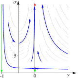
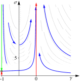
Figure 13: Comparison between expected RG-flow for a double layer system of NTSM (left) and the coupled surfaces of a thin 3D TI film (right).

V.2 General RG flow

We now turn our attention to the complete analysis of RG equations (101) which, in general, describe the case of different carrier density, disorder and interaction strength on the top and bottom surfaces of a 3D TI film. The renormalization of interaction parameters $\gamma_{11}$ and $\gamma_{22}$, Eqs. (103c) and (103d), determines four fixed planes of the RG flow:

• $\gamma_{11}=-1=\gamma_{22}$. Repulsive fixed plane of two decoupled surfaces with only intrasurface Coulomb interaction. This problem has been studied in Ref. Ostrovsky et al., 2010.

• $\gamma_{11}=0$, $\gamma_{22}=-1$ or vice versa. Fixed plane describing a 3D TI film with strongly different surface population. This case in analyzed in Sec. V.2.1 below.

• $\gamma_{11}=0=\gamma_{22}$. Attractive fixed plane. Intrasurface interaction has died out and only intersurface interaction survived. This case is analyzed in Sec. V.2.2 below.

Concerning the repulsive fixed planes, one should keep in mind that the renormalization of interaction amplitudes is suppressed by the small factor $1/\sigma$. Therefore even if the conditions on $\gamma_{11}$ and $\gamma_{22}$ are only approximately fulfilled the behavior in the fixed plane dictates the RG flow in a large temperature/frequency window. RPA-estimates of the bare values of interaction amplitudes can be found in Appendix C.6.

We also remind the reader that the RG equations describing the model with finite-range interaction (and thus the whole crossover between the problem with Coulomb interaction and the non-interacting system) is discussed in Appendix F.

V.2.1 Strongly different surface population

We investigate here the fixed plane of Eqs. (101) in which $\gamma_{11}=0$ and $\gamma_{22}=-1$. (Clearly, the reversed situation $\gamma_{11}=-1$ and $\gamma_{22}=0$ is completely analogous.) Both fixed planes are “saddle-planes” of the RG flow, i.e., they are attractive in one of the $\gamma$-directions and repulsive in the other.

Before analyzing this fixed plane, it is worth explaining why this limit is of significant interest for gate-controlled transport experiments, in particular, those on Bi₂Se₃. As for this material the Fermi energy is normally located in the bulk conduction band, an electrostatic gate is conventionally used to tune the chemical potential into the bulk gap and hence to bring the system into a topologically non-trivial regime. A situation as depicted in Fig. 14 is then believed to arise in a certain range of gate voltages: SteinbergPRB one of the two surfaces (here surface 1) is separated by a depletion region from a relatively thick bulk-surface layer.

Recently, Ostrovsky et al. (2012); Garate and Glazman (2012); Krueckl and Richter (2012) disorder-induced interference corrections for 3D TI bulk electrons have been investigated theoretically: While at small length scales additional symmetries of the Hamiltonian provide non-trivial localization behavior, at sufficiently large scales the usual WAL effect sets in. The strong coupling between electron states in the conducting part of the bulk and at surface 2 does not alter this universal low-energy property. In conclusion, at sufficiently large length scales the symplectic class NL$\sigma$M, Eq. (61), is the adequate description of such a system (under the assumption of negligible tunneling between surface 1 and the conducting part of the bulk).

Since the bulk-surface layer has a much higher carrier density than the carrier density on the spatially separated surface 1 we can expect that $\kappa_{2}\gg\kappa_{1}$. Provided $\kappa_{1}d\ll 1$ the electron-electron interaction on the spatially separated surface 1 is effectively screened out such that $|\gamma_{11}|\approx(\kappa_{1}/\kappa_{2})(1+2\kappa_{2}d)\ll 1$ (see Eq. (9)). Conversely, the effect of screening by electrons on the surface 1 is negligible for Coulomb interaction of the bulk states: $1+\gamma_{22}\approx\kappa_{1}/\kappa_{2}\ll 1$.

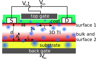
Figure 14: Typical scenario for gate-controlled transport experiments: A topologically protected surface separated from a thick bulk-surface layer.

Substituting $\gamma_{11}=0$ and $\gamma_{22}=-1$ into Eqs. (103), we find that the RG equations in this fixed plane are as follows

$$\rule{0.0pt}{12.91663pt}\rule[-8.61108pt]{0.0pt}{0.0pt}\frac{d\sigma}{dy} =-\frac{2}{\pi}\left\{1-\frac{1}{t}\ln(1+{t})\right\},$$ (109a)

$$\rule{0.0pt}{12.91663pt}\rule[-8.61108pt]{0.0pt}{0.0pt}\frac{dt}{dy} =-\frac{2}{\pi}\frac{1+t}{\sigma}\left\{\frac{1-t}{2}-\frac{1}{t}\ln(1+{t})\right\}.$$ (109b)

They can equivalently be written in terms of conductivities $\sigma_{1}$ and $\sigma_{2}$:

$$\rule{0.0pt}{12.91663pt}\rule[-8.61108pt]{0.0pt}{0.0pt}\frac{d\sigma_{1}}{dy} =-\frac{2}{\pi}\left\{\frac{1}{2}-\frac{\sigma_{2}}{\sigma_{1}}\text{ln}\left[1+\frac{\sigma_{1}}{\sigma_{2}}\right]\right\},$$ (110a)

$$\rule{0.0pt}{12.91663pt}\rule[-8.61108pt]{0.0pt}{0.0pt}\frac{d\sigma_{2}}{dy} =-\frac{1}{\pi}.$$ (110b)

We emphasize that the limit $\gamma_{11}=0$ and $\gamma_{22}=-1$ is very peculiar. Indeed, due to the relation (72), this limit implies that the condition $z_{1}/z_{2}=0$ holds. Equations (109) and (110) are written under assumption that the ratio $t=\sigma_{1}/\sigma_{2}$ is finite in spite of the fact that $z_{1}/z_{2}=0$. In the experiment it corresponds to the case in which $\kappa_{1}/\kappa_{2}\ll 1$ but the ratio $D_{1}/D_{2}\gg 1$ where $D_{s}=\sigma_{s}/4z_{s}$ is the diffusion coefficient.

Equations (110) become decoupled for $\sigma_{1}/\sigma_{2}=0$. Then, as expected, $\delta\sigma_{1}=\frac{1}{\pi}\ln L/l$ (WAL, no interaction on the surface 1) and $\delta\sigma_{2}=-\frac{1}{\pi}\ln L/l$ (WAL and AA due to Coulomb interaction on the surface 2). However, the line $t=0$ is unstable. As one can see from Eq. (109b), due to the very same quantum corrections the initially small parameter $t=\sigma_{1}/\sigma_{2}$ increases under RG. The ultimate limit of the perturbative RG flow is $\sigma\rightarrow 0$ and $t\rightarrow\infty$, see Fig. 15. The scale dependence of $\sigma_{1}$ is non-monotonous; the position of the corresponding maximum is determined by zeros of the right-hand-side of Eq. (110a) shown by a green line in the right panel of Fig. 15.

As has been already emphasized, the perturbative RG equations are sufficient only in the regime of large $\sigma_{s}$. We now discuss the topological effects at small values of conductivities. In the limit $\gamma_{11}=0$, $\gamma_{22}=-1$ the renormalization of $\sigma_{2}$ is exactly independent of the surface 1. Indeed, in the conductivity corrections, the two surfaces influence each other only via mutual RPA screening. In the NL$\sigma$M description the interaction amplitudes in the full action (61) and hence in the propagators (87) (diffusons and cooperons) fully account for this effect. Since the layer 2 includes a single TI surface, we know that $\sigma_{2}$ is topologically protected and flows towards $\sigma_{2}^{*}$ of the order of the quantum of conductance (“interaction-induced criticality” Ostrovsky et al. (2010)). Before this happens, the flow of $\sigma_{1}$ becomes reversed from antilocalizing to localizing, see Eq. (110a). However, since the surface 1 is also topologically protected, its states can not be strongly localized and $\sigma\rightarrow\sigma_{1}^{*}>0$. Thus, both surfaces are at the quantum critical points with conductivities of order $e^{2}/h$. The conclusion concerning the surface 1 is particularly remarkable: even though $\gamma_{11}=0$, there is “intersurface-interaction-induced criticality” on the surface 1.

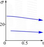
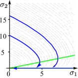
Figure 15: Perturbative RG flow in the fixed plane $\gamma_{11}=0$, $\gamma_{22}=-1$. In the experimentally motivated scenario (Fig. 14), the flow starts at $t=\sigma_{1}/\sigma_{2}\ll 1$. The green line in the right panel is a line of zeros of the right-hand-side of Eq. (110a); it determines the maximum in the RG flow of $\sigma_{1}$.

V.2.2 Attractive fixed plane

According to Eqs. (103c) and (103d), any $\gamma_{ss}\notin\left\{0,-1\right\}$ is renormalized to zero. The $\gamma_{11}=\gamma_{22}=0$ is thus an attractive fixed plane of the general RG flow. The flow within this plane has the form determined by the following RG equations

$$\rule{0.0pt}{12.91663pt}\rule[-8.61108pt]{0.0pt}{0.0pt}\frac{d\sigma}{dy} =-\frac{2}{\pi}\left\{1-\frac{1}{t}\text{ln}\left[1+{t}\right]-{t}\text{ln}\left[1+\frac{1}{t}\right]\right\},$$ (111a)

$$\rule{0.0pt}{12.91663pt}\rule[-8.61108pt]{0.0pt}{0.0pt}\frac{dt}{dy} =-\frac{2}{\pi}\frac{1+t}{\sigma}\left\{\frac{1-t}{2}-\frac{1}{t}\text{ln}\left[1+{t}\right]+{t^{2}}\text{ln}\left[1+\frac{1}{t}\right]\right\},$$ (111b)

or, equivalently,

$$\rule{0.0pt}{12.91663pt}\rule[-8.61108pt]{0.0pt}{0.0pt}\frac{d\sigma_{1}}{dy} =-\frac{2}{\pi}\left\{\frac{1}{2}-\frac{\sigma_{2}}{\sigma_{1}}\text{ln}\left[1+\frac{\sigma_{1}}{\sigma_{2}}\right]\right\},$$ (112a)

$$\rule{0.0pt}{12.91663pt}\rule[-8.61108pt]{0.0pt}{0.0pt}\frac{d\sigma_{2}}{dy} =-\frac{2}{\pi}\left\{\frac{1}{2}-\frac{\sigma_{1}}{\sigma_{2}}\text{ln}\left[1+\frac{\sigma_{2}}{\sigma_{1}}\right]\right\}.$$ (112b)

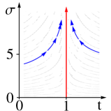
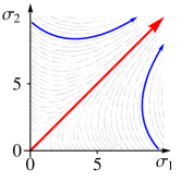
Figure 16: The RG flow in the attractive fixed plane $\gamma_{11}=0=\gamma_{22}$. The zero of Eq. (111b) is displayed by the red line.

Even though the single-surface conductivities $\sigma_{s}$ display non-monotonic behavior within this plane, eventually all quantum corrections are antilocalizing, see Fig. 16. The ratio of conductivities flows to the symmetric situation $t=\frac{\sigma_{1}}{\sigma_{2}}=1$, as has been discussed in Sec. V.1. We reiterate that at the corresponding fixed line the WAL effect is competing with a contribution of the opposite sign due to intersurface interaction. While the WAL wins, the antilocalizing flow is slower than for free electrons, see Eq. (106).

V.2.3 General RG flow

After having analyzed the RG flow in various fixed planes, we briefly discuss the general RG flow. According to Eqs. (101c) and (101d), there is a single attractive fixed point of the overall RG flow – the metallic fixed point with zero intrasurface interaction, $\sigma_{1}=\sigma_{2}\to\infty$ and $\gamma_{11}=\gamma_{22}=0$. On the other hand, for the values of $\gamma_{ss}$ close to $-1$ the corresponding conductivity $\sigma_{s}$ is first subjected to localizing quantum corrections and will thus show a non-monotonic behavior towards antilocalization. There also exists a range of initial parameters for the RG flow for which the conductivity at one surface demonstrates monotonous antilocalizing behavior, while the conductivity in the other surface flows in the described non-monotonous manner.

VI Discussion and experimental predictions

In the preceding Section we have performed a general analysis of the renormalization group flow determined by the RG equations (101). The purpose of the present Section is to apply these results to specific experimentally relevant materials.

VI.1 Parameters

As explained in Sec. II.1, the RG equations (101) apply in the case of the following hierarchy of length scales:

$$l \ll L_{E},$$ (113a)

$$d \ll l.$$ (113b)

In order to deal with $$q \kappa_{s}d\ll 1 s=1 s=2$$-independent interaction amplitudes, an additional requirement occurs in the case for both and :

$$l_{\rm scr}\ll L_{E}.$$ (113c)

In view of condition (113a), the constraint (113c) is fulfilled in the entire diffusive regime if $$l_{\rm scr}\ll l$$.

Further, we have assumed that the intersurface tunneling is negligible; the corresponding condition reads

$$a \ll d.$$ (113d)

In this Section, we will concentrate on the case when the RG scale is set by temperature, $L_{E}=l_{T}$. We recall the definition of the length scales entering the above conditions: $l=\max_{s=1,2}l_{s}$ is the larger mean free path, $l_{T}=\min_{s=1,2}\sqrt{D_{s}/kT}$ the smaller thermal length, $d$ the sample thickness, $a$ the penetration depth, $\kappa_{s}$ the inverse Thomas-Fermi screening length for the surface $s$ and $l_{\rm scr}$ the total screening length for the 3D TI film. The situation in which only one of the two surfaces is in the diffusive regime, while the other one is in the ballistic regime (i.e. $T\tau_{1}\ll 1$ and $T\tau_{2}\gg 2$ or vice versa) is also a conceivable and interesting scenario. However, we do not address it in the present paper.

The effect of intersurface interaction becomes prominent if the sample thickness does not exceed too much at least one of the single surface screening lengths $\kappa_{s}^{-1}$. As discussed above (Sec. V), this condition implies that the bare values of interaction $\gamma_{11}$ and $\gamma_{22}$ are not too close to $-1$.

It is useful to present expressions for the length scales appearing in the conditions (113a)-(113d) in terms of standard parameters characterizing samples in an experiment. For simplicity, we assume $v_{F}^{(1)}=v_{F}^{(2)}$ and $\tau_{1}=\tau_{2}$ in these formulas.

The densities of states (DOS) and inverse screening lengths for the top and bottom surfaces are

$$\nu_{s}=\sqrt{\frac{n_{s}}{\pi v_{F}^{2}}},\qquad\kappa_{s}\equiv\frac{2\pi e^{2}}{\epsilon_{2}}\nu_{s}=2\pi\alpha\sqrt{\frac{n_{s}}{\pi}}$$ (114)

where $n_{s}$ are the corresponding electron densities. If the electron densities for each surface separately are not known, the total density $n_{\text{tot}}=n_{1}+n_{2}$ can be used to estimate the DOS and the screening lengths:

$$\nu_{1}^{2}+\nu_{2}^{2}=\frac{n_{\text{tot}}}{\pi v_{F}^{2}},\qquad\kappa_{1}^{2}+\kappa_{2}^{2}=\left(2\pi\alpha\right)^{2}\frac{n_{\text{tot}}}{\pi}.$$ (115)

The mean free path can be expressed as

$$l=v_{F}\tau_{tr}=\frac{\sigma}{\pi v_{F}\left(\nu_{1}+\nu_{2}\right)}.$$ (116)

The thermal length in the diffusive regime is given by

$$l_{T}=\sqrt{\frac{D}{kT}}=\sqrt{\frac{v_{F}l}{2kT}}=\sqrt{\frac{\sigma}{kT2\pi\left(\nu_{1}+\nu_{2}\right)}}$$ (117)

Hence, the condition (113a) is fulfilled for temperatures

$$kT\ll kT_{\text{Diff}},$$ (118)

where

$$kT_{\text{Diff}}=\frac{v_{F}}{2l}=\frac{1}{\sigma[e^{2}/h]}\left(\frac{v_{F}^{2}}{2}\right)2\pi(\nu_{1}+\nu_{2})$$ (119)

is the temperature scale at which the diffusion sets in.

In order to obtain $l_{\rm scr}$ entering Eq. (113c), we have to consider the full (inter- and intrasurface) Coulomb interaction, see Appendix B. As explained in Sec.  II.2 it is only a meaningful quantity provided $\kappa_{s}d\ll 1$. Taking into account the influence of the surrounding dielectrics, we find

$$l_{\rm scr}=\frac{\epsilon_{1}+\epsilon_{3}}{2\epsilon_{2}}\frac{1}{\kappa_{1}+\kappa_{2}}.$$ (120)

When deriving Eq. (120), we assumed for simplicity that $\epsilon_{2}\lesssim\epsilon_{1}+\epsilon_{3}$. Regarding the experimental setups discussed in Sec. VI.2, this condition is well fulfilled for Bi₂Se₃ but only marginally for HgTe. Thus in the latter case Eq. (120) should be considered as a rough estimate.

Finally, to check the validity of the condition (113d), one needs to know the value of the penetration depth $a$. The latter can be estimated from the condition

$$\frac{v_{F,\perp}p_{\perp}}{\Delta_{\text{bulk}}}\sim 1,$$ (121)

where $p_{\perp}\sim 1/a$ denotes typical momenta perpendicular to the surface. Provided $v_{F,\perp}\sim v_{F}$, it yields

$$a\sim\frac{v_{F}}{\Delta_{\text{bulk}}}.$$ (122)

We are now going to consider two exemplary materials for 3D TIs: Bi₂Se₃ and strained HgTe. We shall estimate numerically all the relevant parameters and present characteristic plots for temperature dependence of conductivities.

VI.2 Exemplary 3D TI materials

VI.2.1 Bi₂Se₃

Fermi velocity	$v_{F}\sim 5\times 10^{5}$m/s
Bulk gap	$\Delta_{\text{bulk}}\sim 0.3$ eV
Sample thickness	$d\sim$ 10 nm
Dielectric properties	Coat: $\epsilon_{1}\sim 1$ 3D TI (Bi2Se3): $\epsilon_{2}\sim 100$ Substrate (SrTiO3): $\epsilon_{3}\sim 10^{3}-10^{4}$
Carrier density	$n_{\text{tot}}\sim 3\times 10^{12}$ cm-2
Mobility	$\mu_{el}\sim 100\dots 1000$ cm${}^{2}/$V$\cdot$s
Sheet resistance	$1/\sigma\sim 0.097\,h/e^{2}$ at $T\sim 50$ mK
Effective coupling	$\alpha\sim 4\times 10^{-2}$
Chemical potential	$\mu_{1}^{2}+\mu_{2}^{2}=\left(0.2\,\text{eV}\right)^{2}$
Penetration depth	$a\sim 1$ nm
Mean free path	$l\sim 24\dots 34$ nm
Diff. temperature	$T_{\text{Diff}}\sim 80\dots 57$ K
Screening length	$\kappa_{1}^{2}+\kappa_{2}^{2}\sim\left(37\text{ nm}\right)^{-2}$
Scr. length (total)	$l_{\rm scr}\sim 132\dots 186\text{ nm},\;\text{for}\;\epsilon_{3}=10^{3}$
Bare interaction (RPA)	top surface: $\gamma_{11}\sim-0.6\dots-1$ bottom surface: $\gamma_{22}\sim-0.6\dots 0$

Table 1: Experimental values of sample parameters at the point of the minimal carrier density and associated length scales for transport experiments on Bi₂Se₃ films of Refs. [Chen et al., 2011; Li, 2012]. The dots “$\dots$” separate values for the symmetric ($n_{1}=n_{2}$) and totally asymmetric ($n_{1}=n_{\text{tot}},n_{2}=0$) cases. The bare interaction amplitudes are estimated in the random phase approximation (RPA).

Bi₂Se₃ is currently the most conventional material for experimental realization of the 3D TI phase. Typical experimental data (extracted from the point of the minimal conductance in Refs. Chen et al., 2011; Li, 2012) is summarized in the upper part of Table 1. Using Eqs. (114) – (122) we can estimate the hierarchy of length scales (lower part of the same Table). One can see that all of the requirements of validity for our theory are fulfilled for length scales above $l_{\rm scr}$ [temperatures below $T_{\max}=2.6\dots 1.9$K, see condition (113c).]

From the experimental data, the ratio of carrier densities is not known. Therefore, we show in Fig. 17 the expected temperature dependence of total conductivity for various values of this ratio. Clearly, the behavior strongly differs from the case of decoupled surfaces (dashed line). First, the slope of $d\sigma/d\ln T$ is considerably smaller. Second, one observes a clear curvature of the dependence $\sigma(\ln T)$ which is a manifestation of the non-monotonicity. (For the parameters used in the plot the minimum of $\sigma$ occurs at still lower temperatures.) This curvature is especially pronounced for strongly different surfaces.

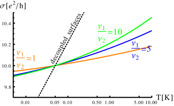
Figure 17: Theoretical prediction for the temperature dependence of the total conductivity in thin Bi₂Se₃ films.

It should be mentioned that the substrate used in Ref. Chen et al., 2011 has a strongly temperature-dependent dielectric function $\epsilon_{3}$ since SrTiO₃ approaches a ferroelectric transition at low temperatures. This could result in a temperature dependence of effective gate voltage and consequently of carrier density. The resulting classical temperature dependence of conductivity (and interaction constants) would mask the quantum effects described in our analysis. However, in the presence of the gating field, the temperature dependence of $\epsilon_{3}$ saturates at low temperatures. This motivates the presentation in Fig. 17 where we assumed independent of temperature $\epsilon_{3}=1000$.

VI.2.2 Strained HgTe

Fermi velocity	$v_{F}\sim 5\times 10^{5}$m/s
Bulk gap	$\Delta_{\text{bulk}}\sim 0.022$ eV
Sample thickness	$d\sim$ 70 nm
Dielectric properties	Coat: $\epsilon_{1}\sim 1$ 3D TI (HgTe): $\epsilon_{2}\sim 21$ Substrate (CdTe): $\epsilon_{3}\sim 10$
Carrier density	top surface: $n\sim 4.8\times 10^{11}$ cm-2 bottom surface: $n\sim 3.7\times 10^{11}$ cm-2
Mobility	$\mu_{el}\sim 34000$ cm2/V$\cdot$s
Sheet resistance	$1/\sigma\sim 0.04\,h/e^{2}$ at $T=50$ mK
Effective coupling	$\alpha\sim 0.21$
Chemical potential	top surface: $\mu_{1}\sim 0.08$ eV bottom surface: $\mu_{2}\sim 0.07$ eV
Penetration depth	$a\sim 15$ nm
Mean free path	$l\sim 108$ nm
Diff. temperature	$T_{\text{Diff}}\sim 18$ K
Screening length	top surface: $\kappa_{1}^{-1}\sim 19.53$ nm bottom surface: $\kappa_{2}^{-1}\sim 22.24$ nm
Bare interaction (RPA)	top surface: $\gamma_{11}\sim-0.893$ bottom surface: $\gamma_{22}\sim-0.878$

Table 2: Typical experimental values for transport experiments on HgTe films of Refs. [BaarsSorger1972, ; Brüne et al., 2011].

Another very promising 3D TI material is strained HgTe. The presence of Dirac-like surface states was experimentally confirmed by the odd series of QHE plateaus, as well as by ARPES Brüne et al. (2011). While the transport experiment indicates dominant surface conduction, the extracted carrier density appears to be too large for a pure surface theory with linear spectrum, yielding the value of the chemical potential $\mu$ larger than the gap $\Delta_{\rm bulk}$, see Table 2. (The role of the bulk conduction band as well as the parabolic bending of the dispersion was also discussed within an independent magneto-optical study by the same experimental group. Hancock et al. (2011)) Thus, it remains to be clarified under what experimental conditions the strained HgTe sample is in the true TI regime (i.e., the bulk contribution to transport is negligible). Notwithstanding this point and motivated by the excellent surface transport data, we apply our theory to the HgTe experiment, see Fig. 18. In spite of the considerable thickness of the probe, the effect of intersurface interaction is clearly visible: the slope of $d\sigma/d\ln T$ is considerably smaller than it is expected for decoupled surfaces.

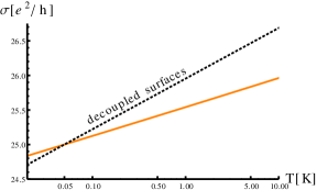
Figure 18: Theoretical prediction for the temperature dependence of the total conductivity in thin films of strained HgTe.

VI.3 Hallmarks of surface transport and interactions

We briefly summarize now our most salient predictions for experimental signatures of surface transport in 3D TI with an intersurface interactions.

• As already exploited in 3D TI experiments, Chen et al. (2011) the magnetoconductance formula Hikami et al. (1980) for the total conductivity is

  $$\delta\sigma\left(B\right)=-\frac{e^{2}}{2\pi h}\sum_{s=1,2}\left[\psi\left(\frac{1}{2}+\frac{B^{(s)}_{\phi}}{B}\right)-\ln\left(\frac{B^{(s)}_{\phi}}{B}\right)\right],$$ (123)

  where the characteristic magnetic field $B^{(s)}_{\phi}=\hbar/(4eD_{s}^{(s)}\tau^{(s)}_{\phi})$ is determined by the diffusion coefficient $D_{s}^{(s)}$ and the phase breaking time $\tau^{(s)}_{\phi}$ for the surface $s$. The function $\psi$ denotes the digamma function here.

• The characteristic effect of intersurface interaction is the non-monotonous temperature dependence of conductivity (see Fig. 19, top). It may happen that in experimentally accessible temperature window this effect manifests itself only as a deviation of the conductance slope

  $$\delta\sigma\left(T\right)={\;\frac{e^{2}}{h}}c\ln T$$ (124)

  from the value $c=1/\pi$ characteristic for two decoupled surfaces accompanied by some bending of the curve $\sigma(\ln T)$, see Figs. 17 and 18. The ultimate low-$T$ behavior of the coupled system is always antilocalizing and following the universal law

  $$\delta\sigma\left(T\right)={\;\frac{e^{2}}{\pi h}}\left(1-2\ln 2\right)\ln T.$$ (125)

  However, depending on the parameters, this asymptotics may become valid at very low temperatures only.

• The strength of intersurface interaction is governed by the parameters $\kappa_{1}d$ and $\kappa_{2}d$, where $\kappa$ is the screening length. Therefore, in contrast to usual, single surface conductivity corrections, the predicted effect strongly depends on the carrier density (see Fig. 19, bottom).

It is also possible to access the intersurface induced quantum corrections in the frequency dependence of the AC conductivity (by the simple replacement $T\rightarrow\omega$ in $\delta\sigma\left(T\right)$ if $\omega\gg T$).

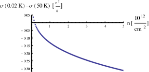
Figure 19: Top: Conductivity corrections for low carrier concentration. The total electron concentration in units of $10^{12}\text{cm}^{-2}$ is equal to $0.55,0.48,0.41,0.34,0.27$ from bottom to top. The characteristic non-monotonous behavior is clearly seen; deviations from the behavior of decoupled surfaces are very strong. Bottom: Carrier-density dependence of conductivity corrections. The non-trivial dependence is entirely due to the intersurface interaction: in the case of the decoupled surfaces, the conductivity correction would be constant as a function of density, $\sigma\left(0.02K\right)-\sigma\left(50K\right)\approx-2.49e^{2}/h$. We used the values of the parameters $d$, $v_{F}$ and $\alpha$ as in Table 1 for Bi₂Se₃. Further, we assumed the case of equal surfaces ($n_{tot}=2n$) and $T_{\text{Diff}}=1/2\tau=50K$.

VII Conclusions

In this paper, we have investigated interference and interaction effects in the surface state conductivity of 3D topological insulator slabs. We have taken into account the electron-electron interaction within the top and bottom surfaces of a slab and between them. These two surfaces were in general assumed to be characterized by different carrier densities and scattering rates, and by asymmetric dielectric environment.

Our field-theoretical analysis was based on the interacting non-linear sigma model approach describing the system at length scales above the mean free path. We demonstrated how this effective theory can be obtained from the non-Abelian bosonization. In particular, we have shown that upon inclusion of potential disorder the Wess-Zumino term generates a local expression for the $\mathbb{Z}_{2}$ theta term. The appearance of this topological term is the hallmark of the Dirac surface states; it is absent in conventional 2D metals of the same symmetry class. We have further analyzed the $\mathbf{U}(1)$-gauged sigma model that describes a coupling to the external electromagnetic field. This has allowed us to connect the physical linear-response characteristics of the problem and the sigma-model coupling constants. We have also analyzed the effect of breaking of time-reversal symmetry, namely, the anomalous quantum Hall effect of Dirac electrons.

It is worth emphasizing that our theory treats the general situation of potentially strong interactions and thus went beyond perturbation theory. We have thus developed the Fermi liquid theory of the strongly correlated double layer system in the ballistic and diffusive regime.

We renormalized the interacting NL$\sigma$M of the two surfaces in the one-loop approximation and obtained the RG equations, Eq. (101). This way we have determined the temperature (or else, frequency, or length scale) dependence of the conductivities of both surfaces. The RG is controlled by a large conductivity, $k_{F}l\gg 1$. Our calculations are exact in the singlet interaction amplitudes, while contributions due to a repulsive Cooper interaction are parametrically small and can be neglected.

Inspecting the RG equations, we showed that intersurface interaction is relevant in the RG sense and the limiting case of decoupled surfaces is therefore unstable. The rich flow diagram has been analyzed in detail. For fully decoupled surfaces the system flows into an intermediate-coupling fixed point (“interaction-induced criticality”). This point is, however, unstable with respect to the intersurface coupling. The flow is then towards a single attractive fixed point which is “supermetallic”, $\sigma\to\infty$, and at which even originally different surfaces have the same transport properties, $\sigma_{1}=\sigma_{2}$, see Figs. 11 and 16. Further, this fixed point is characterized by vanishing intrasurface and finite intersurface interaction. Typically, this fixed point is reached via a characteristic non-monotonous temperature dependence of conductivity.

Our perturbative results are equally applicable to weak topological insulatorRingel et al. (2012); KobayashiOhtsukiImura13 thin films and to non-topological double layer systems with spin-orbit interaction. For the latter type of structures, we have also discussed the difference compared to the strong TI films which is in non-perturbative topological effects, see a comparison of the flow diagrams in Fig. 13. While in the TI case these effects lead to a topological protection of the surface states from Anderson localization, a conventional (non-topological) double layer system undergoes a metal-insulator transition which is tuned by the ratio of interlayer distance and screening length.

Finally, we have estimated parameters and presented explicit predictions for the temperature dependence of the conductivity for typical experimental setups based on Bi₂Se₃ and strained HgTe materials.

Before closing, we discuss perspectives for further research. First, experimental studies of temperature dependence of conductivity of 3D topological insulators for different positions of chemical potentials would be highly useful. A comparison of such experimental data with our theoretical predictions would allow one to judge whether the system is in the truly topological phase. Second, more work is needed on effects of local breaking of time-reversal symmetry in TI slabs. Third, it is known that Coulomb interaction in electronically decoupled double-layer systems induces a finite but typically small transconductance $\sigma_{12}$.Solomon et al. (1989); Gramila et al. (1991); Carrega et al. (2012); Schütt et al. (2013) However, the side walls of 3D TI films connect the two major surfaces, which might be a serious obstacle for performing Coulomb drag experiments. Fourth, in view of recent experimental progress,Wray et al. (2010) it would be interesting to perform an RG analysis for a superconducting counterpart of the system that we have explored, namely, for surface states of a 3D topological superconductor with spin-orbit interaction (class DIII).FosterYuzbashyan2012

VIII Acknowledgements

We thank J. Smet, Y.Q. Li, A. Finkel’stein, M. Schütt and U. Briskot for useful discussions. The work was supported by BMBF, DAAD, DFG SPP 1666, RAS programs “Quantum mesoscopic and disordered systems”, “Quantum Physics of Condensed Matter”, “Fundamentals of nanotechnology and nano materials”, RFBR grants No. 11-02-12126 and No. 12-02-00579, Russian President grant No. MK-4337.2013.02, and by the Russian Ministry of Education and Science under contract No. 8678.

Appendix A Non-Abelian bosonization and the topological term

In this appendix we include more detailed calculations concerning non-Abelian bosonization, the gauged WZNW model and the topological term $S^{(\theta)}$. For brevity, we omit the surface index $s$ in this appendix.

A.1 Gauged WZNW model

The Wiegmann-Polyakov formulaPolyakov and Wiegmann (1983) allows the inclusion of smooth $\mathfrak{o}\left(2_{\tau}\times 2N_{M}\times N_{R}\right)$ gauge fields $A_{\mu}$. A generalization to potentially topological gauge potentials can be found in Refs. Faddeev, 1976; Gerasimov, 1993; Losev et al., 1995; Smilga, 1996. The gauged WZNW model is given as Faddeev (1976); Gerasimov (1993); Losev et al. (1995); Smilga (1996)

$$S\left[O,A_{\mu}\right]=-\frac{1}{16\pi}\int\limits_{\textbf{{x}}}\text{tr}\left(O^{T}D_{\mu}O\right)\left(O^{T}D_{\mu}O\right)$$ (126a)

$$+\frac{i\epsilon_{\mu\nu\rho}}{24\pi}\int\limits_{\textbf{{x}},w}\text{tr}\left[\left(O^{T}D_{\mu}O\right)\left(O^{T}D_{\nu}O\right)\left(O^{T}D_{\rho}O\right)\right]$$ (126b)

$$-\frac{i\epsilon_{\mu\nu\rho}}{16\pi}\int\limits_{\textbf{{x}},w}\text{tr}\left[F_{\mu\nu}\left(O^{T}D_{\rho}O+D_{\rho}OO^{T}\right)\right],$$ (126c)

where we introduced $D_{\mu}=\partial_{\mu}+\left[A_{\mu},\cdot\right]$ and $F_{\mu\nu}=\left[D_{\mu},D_{\nu}\right]$. In the main text, we were mostly interested in $\mathbf{U}\left(1\right)$ gauge fields $A_{\mu}=i\hat{A}^{T}\frac{1+\tau_{y}}{2}-i\hat{A}\frac{1-\tau_{y}}{2}$. (In this appendix, the electron charge is absorbed into the vector potential.)

To obtain the Wiegmann-Polyakov formula, one can use the following identity Smilga (1996)

$$\eqref{eq:GammaOA} =\frac{i}{24\pi}\Gamma\left[O\right]$$

$$-\frac{i}{8\pi}\int_{\textbf{{x}},w}\epsilon_{\mu\nu\rho}\partial_{\mu}\text{tr}\left[OA_{\nu}O^{T}A_{\rho}\right.$$

$$\hskip 56.9055pt\left.+A_{\nu}\left(O^{T}\partial_{\rho}O+\partial_{\rho}OO^{T}\right)\right]$$

$$+\frac{i\epsilon_{\mu\nu\rho}}{16\pi}\int_{\textbf{{x}},w}\text{tr}\left[F_{\mu\nu}\left(O^{T}D_{\rho}O+D_{\rho}OO^{T}\right)\right].$$ (127)

While the last integral in Eq. (127) compensates the term (126c), the total derivative term yields the Wiegmann-Polyakov formula provided $A_{\mu}$ is not singular:

$$S\left[O,A_{\mu}\right] =S\left[O\right]+$$

$$+\frac{1}{8\pi}\int_{\textbf{{x}}}\text{tr}\left[A_{\mu}\left(O\partial_{\mu}O^{T}+O^{T}\partial_{\mu}O\right)\right.$$

$$\;+A_{\mu}O^{T}A_{\mu}O-A_{\mu}^{2}-i\epsilon_{\nu\rho}OA_{\nu}O^{T}A_{\rho}$$

$$\;\left.-i\epsilon_{\nu\rho}A_{\nu}\left(O^{T}\partial_{\rho}O+\partial_{\rho}OO^{T}\right)\right]$$ (128)

$$=S\left[O\right]+$$

$$+\frac{1}{8\pi}\int_{\textbf{{x}}}\text{tr}\left[A_{-}\left(O\partial_{+}O^{T}\right)+A_{+}\left(O^{T}\partial_{-}O\right)\right.$$

$$\left.+A_{+}O^{T}A_{-}O-A_{+}A_{-}\right].$$ (129)

Here we have introduced the (anti-)holomorphic combination of gauge potentials $A_{\pm}=A_{x}\pm iA_{y}$. In the case of topological gauge potentials, the integral over the total derivative yields also a contribution from the Dirac string.

Equation (129) is a very powerful result. In particular, it justifies a posteriori the bosonization rules (27a) and (27b). Also, it follows immediately from expression (128) that after disorder-induced symmetry breaking ($O\rightarrow Q=Q^{T}$) the gauge-field-dependent contributions from the topological term vanish.

Further, one can use Eq. (129) to determine the prefactor of the kinetic term in the AII NL$\sigma$M, Eq. (43). As explained in the main text, soft rotations $O^{T}_{\text{soft}}OO_{\text{soft}}$ of the WZNW fields $O$ are not affected by disorder induced masses, Eq. (32). The effective action for topologically trivial Goldstone modes contains

$$S_{\rm eff,kin}\left[\Phi_{\mu}\right] =\frac{1}{8\pi}\int_{\textbf{{x}}}\left\langle\text{tr}\left[\Phi_{+}O^{T}\Phi_{-}O-\Phi_{+}\Phi_{-}\right]\right\rangle$$

$$-\frac{1}{2}\left\langle\left(\int_{\textbf{{x}}}\text{tr}\left[\Phi_{+}j_{-}+\Phi_{-}j_{+}\right]\right)^{2}\right\rangle,$$ (130)

where $j_{\pm}$ are the (bosonic) currents, $\left\langle\dots\right\rangle$ denotes average with respect to the full bosonic theory (including the mass terms) and $\Phi_{\pm}=O_{\text{soft}}\partial_{\pm}O_{\text{soft}}^{T}$. To the leading order, the average can be calculated close to the saddle point. Exploiting the equivalence of bosonic and fermionic theories one can equally evaluate $\left\langle\dots\right\rangle$ using the fermionic fields at SCBA level. At $|\mu|\tau\gg 1$ the major contribution comes from the second line of Eq.(130), which, taking the vertex corrections into account, yields the correct prefactor (i.e. the conductivity) of the kinetic term in Eq. (43).

A.2 Instanton configuration

We define the following four dimensional unit vector

$$\underline{a} \equiv \left(a_{0},a_{1},a_{2},a_{3}\right)$$

$$\equiv \frac{1}{|\vec{x}-\vec{x}^{\prime}|^{2}+\lambda^{2}}\left(2\lambda\left(\vec{x}-\vec{x}^{\prime}\right),|\vec{x}-\vec{x}^{\prime}|^{2}-\lambda^{2}\right),$$

where the 1+2 vector $\vec{x}-\vec{x}^{\prime}\equiv\left((1-w)/w,\textbf{{x}}-\textbf{{x}}^{\prime}\right)$ contains the extension parameter and the real-space coordinates. It describes a topological excitation at position $\left(1,\textbf{{x}}^{\prime}\right)$ in a three-dimensional base space. With the help of the vector $\underline{a}$ we can define the following extended field configuration

$$\tilde{O}_{\rm inst}=\left(\begin{array}[]{cccc}-a_{0}i\tau_{y}+a_{3}&0&a_{1}+a_{2}i\tau_{y}&0\\ 0&\textbf{{1}}&0&0\\ a_{1}-a_{2}i\tau_{y}&0&-a_{0}i\tau_{y}-a_{3}&0\\ 0&0&0&-\textbf{{1}}\end{array}\right).$$ (131)

For $a_{0}=0$, i.e. on the physical space $w=1$, $\tilde{O}_{inst}$ is a symmetric matrix and characterizes the two-dimensional instanton. The choice of the extension is arbitrary, but, as has been stressed in the main text, the $\tilde{O}_{\rm inst}$ field has to leave the diffusive saddle-point manifold for some subinterval $w\in I\subseteq\left(0,1\right)$. For $w\rightarrow 0$ the extended field $\tilde{O}_{\rm inst}$ satisfies the boundary condition $\tilde{O}\left(\textbf{{x}},w=0\right)=\Lambda={\rm const}$.

We are now in the position to insert the instanton configuration into the WZNW-term. After tracing out the matrix degrees of freedom this leads to

$$iS^{(\theta)} = \frac{-i}{6\pi}\int_{x,w}\epsilon_{\mu\nu\lambda}\Bigl{(}\epsilon_{abc}\;a_{a}\partial_{\mu}a_{b}\partial_{\nu}a_{c}\partial_{\lambda}a_{0}$$ (132)

$$- \epsilon_{abd}\;a_{a}\partial_{\mu}a_{b}\partial_{\nu}a_{0}\partial_{\lambda}a_{d}$$

$$+ \epsilon_{cda}\;a_{a}\partial_{\mu}a_{0}\partial_{\nu}a_{c}\partial_{\lambda}a_{d}$$

$$- \epsilon_{cdb}\;a_{0}\partial_{\mu}a_{b}\partial_{\nu}a_{c}\partial_{\lambda}a_{d}\Bigr{)}$$

$$= i\pi.$$

Here the last line is obtained by a straightforward calculation. We have thus shown that the topological term distinguishes between the trivial and the non-trivial sectors as it acquires on them the values $0$ and $i\pi\;(\text{mod }2\pi i)$, respectively.

Appendix B Effect of dielectric environment on Coulomb interaction

B.1 Electrostatic Potential and Single Particle Effects

As has been stated above the experimental setup consists of a sandwich of (at least) three different dielectrics (see figure 1). We define the $z$-axis to be perpendicular to the two surfaces. The sandwich consists of the coating material with a dielectric constant $\epsilon_{1}$ (for $d/2<z$), the topological insulator film with a dielectric constant $\epsilon_{2}$ (for $-d/2\leqslant z\leqslant d/2$), and the substrate with a dielectric constant $\epsilon_{3}$ (for $z<-d/2$). Taking these different dielectric properties into account, we here present the expression for the Coulomb potential which generalizes Eq. (4).

By the method of mirror charges, one can deriveProfumo2010 ; Katsnelson2011 ; Carrega et al. (2012) the electrostatic potential induced by a single point charge $e$ located at $\left(\textbf{{x}}_{0},z_{0}\right)=\left(0,0,z_{0}\right)$ inside the middle region of the sandwich ($z,z_{0}\in\left[-\frac{d}{2},\frac{d}{2}\right]$):

$$\Phi\left(\textbf{{x}},z,z_{0}\right) = \frac{e}{\epsilon_{2}}\bigg{[}\frac{1}{\sqrt{\textbf{{x}}^{2}+\left(z-z_{0}\right)^{2}}}$$ (133)

$$+ r_{23}^{-1}\mathcal{F}\left(\textbf{{x}},d+\left(z+z_{0}\right)\right)$$

$$+ r_{21}^{-1}\mathcal{F}\left(\textbf{{x}},d-\left(z+z_{0}\right)\right)$$

$$+ \mathcal{F}\left(\textbf{{x}},z-z_{0}\right)$$

$$+ \mathcal{F}\left(\textbf{{x}},-\left(z-z_{0}\right)\right)\bigg{]},$$

where

$$\mathcal{F}\left(\textbf{{x}},z\right)=\sum_{k=1}^{\infty}\frac{\left(r_{21}r_{23}\right)^{k}}{\sqrt{\textbf{{x}}^{2}+\left(z-2dk\right)^{2}}}.$$ (134)

and the ratios

$$r_{21}\equiv\frac{\epsilon_{2}-\epsilon_{1}}{\epsilon_{2}+\epsilon_{1}};\qquad r_{23}\equiv\frac{\epsilon_{2}-\epsilon_{3}}{\epsilon_{2}+\epsilon_{3}}$$

were introduced. If one of these ratios vanishes, the textbook limit of two dielectric half-planes follows. Fourier transformation of the x coordinates yields

$$\Phi\left(\textbf{{q}},z,z_{0}\right) = \frac{2\pi e}{q\epsilon_{2}}\bigg{[}e^{-|z-z_{0}|q}+\frac{e^{-2dq}}{1-r_{21}r_{23}e^{-2dq}}\times$$ (135)

$$\times \Big{(}r_{21}e^{(d+z+z_{0})q}+r_{23}e^{(d-z-z_{0})q}$$

$$+2r_{21}r_{23}\cosh((z-z_{0})q)\Big{)}\bigg{]}.$$

We consider now 3D TI surface states: the charges are located at a typical distance $a\sim v_{F}/\Delta_{\rm bulk}$ (the penetration depth) from the boundaries $z=\pm\frac{d}{2}$. The consequences of the general expression (135) on the 3D TI surface states are twofold.

First, there is a single particle effect, stemming from the interaction of the charged particles with their own mirror charges. The associated electrostatic energy is incorporated in the chemical potential in the main text and can be expressed as

$$\Delta\mu_{1} = \frac{e}{2}\Phi^{{\rm reg}}\left(0,\frac{d}{2}-a,\frac{d}{2}-a\right)$$

$$= \frac{e^{2}}{4\epsilon_{2}}\left[\frac{r_{21}}{a}-\frac{r_{21}+r_{21}^{-1}+2}{d}\ln\left(1-r_{21}r_{23}\right)\right].$$

The analogous shift of the chemical potential at the second surface $\Delta\mu_{2}$ is easily obtained by interchanging $r_{21}\leftrightarrow r_{23}$. The superscript ^reg indicates that selfinteraction of the charges is subtracted. In the second term we used the approximation $a\ll d$. The first term, i.e. the interaction with the nearest mirror charge, is typically the dominating contribution $\Delta\mu_{1}\approx\alpha_{2}r_{21}/4\Delta_{\rm bulk}$.

Second, the electrostatic energy associated with two-particle interaction is the quantity $\underline{U}_{0}$ entering $S_{\rm int}$ in Eq. (16). This leads to the interaction parameters analyzed below.

B.2 Interaction parameters

The interaction parameters are obtained by placing a test charge into Eq. (135). We will present this effective Coulomb interaction in the surface space. The terms induced by intersurface interaction contain a factor $\exp(-qd)$ ($q$ takes values between the IR and UV cutoffs, $q\in\left[L_{E}^{-1},l^{-1}\right]$). As a result we have to distinguish between the following two cases.

In the first case the momenta are large ($qd\gg 1$) throughout our RG-procedure if $dL^{-1}>1$ or for part of it if $d\in\left[l,L\right]$. Then the two surfaces become decoupled and

$$\underline{U}_{0}=\frac{2\pi}{q}\left(\begin{array}[]{cc}\frac{2}{\epsilon_{2}+\epsilon_{1}}&0\\ 0&\frac{2}{\epsilon_{2}+\epsilon_{3}}\end{array}\right).$$ (137)

(Here and in all subsequent appendices we drop the electron charge, it is formally included into a redefinition of $\epsilon_{1},\epsilon_{2},\epsilon_{3}$.)

In the second case the momenta are small $qd\ll 1$. As we shall be interested in the low-energy theory, we keep only the Fourier transformed terms which are not vanishing in the limit of small transfered momentum $qd\rightarrow 0$. All others are irrelevant in the RG-sense. This way we obtain the true long-range Coulomb part

$$\underline{U}_{C}=\frac{2}{\epsilon_{1}+\epsilon_{3}}\frac{2\pi}{q}\left(\begin{array}[]{cc}1&1\\ 1&1\end{array}\right).$$ (138)

As expected, it does no longer depend on $\epsilon_{2}$. The limit we considered is the large-distance behavior in which the dominant part of the electric field lines lives in the dielectrics surrounding the film.

There are other contributions which do not vanish in the $qd\rightarrow 0$ limit. These are short range interaction amplitudes introduced by the finite thickness of the film:

$$\underline{F}^{(d)} = -\frac{2\pi}{\epsilon_{2}}d\left(\begin{array}[]{cc}0&1\\ 1&0\end{array}\right)$$ (144)

$$-\frac{4\pi}{\epsilon_{1}+\epsilon_{3}}d\left[F_{\rm symm}\left(\begin{array}[]{cc}1&1\\ 1&1\end{array}\right)+\underline{F}_{M}\right].$$

Here we have defined the scalar

$$F_{\rm symm}=\left(\epsilon_{2}-\epsilon_{1}\right)\left(\epsilon_{2}-\epsilon_{3}\right)\left\{\frac{1}{2\epsilon^{2}_{2}}+\frac{1}{\epsilon_{2}\left(\epsilon_{1}+\epsilon_{3}\right)}\right\}$$ (145)

and the matrix

$$\underline{F}_{M}=\frac{1}{2\epsilon_{2}^{2}}\left(\begin{array}[]{cc}\left(\epsilon_{2}+\epsilon_{1}\right)\left(\epsilon_{2}-\epsilon_{3}\right)&\epsilon^{2}_{2}-\epsilon_{1}\epsilon_{3}\\ \epsilon^{2}_{2}-\epsilon_{1}\epsilon_{3}&\left(\epsilon_{2}-\epsilon_{1}\right)\left(\epsilon_{2}+\epsilon_{3}\right)\end{array}\right),$$ (146)

which both vanish in the limit of $\epsilon_{1}=\epsilon_{2}=\epsilon_{3}$. In summary, for coupled surface we can write $\underline{U}_{0}=\underline{U}_{C}+\underline{F}^{(d)}$.

The derivation of the above equations includes some subtleties. First, we derived the electric field configuration for a single point charge. Thus, in particular, we did not consider the metallic surfaces between the dielectrics. As in the theory of conventional metals, their effect will be incorporated in the field theoretical description of the model (Appendix C). Second, we used the potential (135) derived for charged particles at position $z,z_{0}$ and then moved them on the surface between the dielectrics from inside of the TI film ($z_{0}=\pm d/2\mp a\approx\pm d/2$ and equally for $z$). This requires that the (macroscopic) electrostatic theory of continuous, homogeneous dielectrics can be applied to electrons located at a distance $a$ from the boundary. This is justified, as we are interested in the long-range behavior of the electric field. Furthermore, for Bi₂Se₃ it is known that $a$ is of the order of a few nanometers Linder et al. (2009); Zhang et al. (2010), hence one order of magnitude larger than the atomic scale.

Appendix C Clean Fermi liquid

In this appendix we present the formal resummation of scattering amplitudes following references Nozieres and Luttinger, 1962; Abrikosov et al., 1963; Lifshitz et al., 1980. We first consider the short range (one-Coulomb-line-irreducible) part of the singlet channel (see also Eq. (50))

$$\Gamma^{1-2}_{ss^{\prime}}=\Gamma^{1}_{ss^{\prime}}-\Gamma^{2}_{ss}\delta_{ss^{\prime}}\;,$$ (147)

and include the long-range, one-Coulomb-line-reducible, diagrams ($\Gamma^{0}$) later on.

C.1 Resummation of interaction amplitudes

The first step is to single out the subset of particle-hole-section irreducible diagrams $I^{1-2}$. The total interaction amplitude as a matrix in the surface space and in 2+1-momentum space is given by the Dyson equation

$$\underline{\Gamma}^{1-2}\left(K\right)=\underline{I}^{1-2}-\underline{I}^{1-2}\underline{R}\left(K\right)\underline{\Gamma}^{1-2}\left(K\right)$$ (148)

(Matrix multiplication includes momentum integral $\int_{\textbf{{p}}}$and a Matsubara sum $T\sum_{n}$.)

The matrix

$$\left[\underline{R}\left(K\right)\right]_{PP^{\prime},ss^{\prime}} =\delta_{ss^{\prime}}\delta_{PP^{\prime}}R_{s,P}\left(K\right),$$ (149)

$$R_{s,P}\left(K\right) \equiv G_{s}\left(P\right)G_{s}\left(P+K\right)$$ (150)

describes particle-hole bubbles and in the singlet channel. This matrix is diagonal in both 2+1 momentum and surface space: As we explained in the main text, it is sufficient to keep only intrasurface bubbles in the assumed case of uncorrelated disorder. In the presence of generic interaction, the quantity $\underline{R}_{s,P}\left(K\right)$ can be represented as

$$R_{s,P}\left(K\right) = R_{s,P}^{\omega}+\Delta_{{s,P}}\left(K\right)$$ (151)

$$= R_{s,P}^{q}+\tilde{\Delta}_{s,P}\left(K\right).$$ (152)

Here $R_{s,P}^{\omega}$ ($R_{s,P}^{q}$) are called regular (static) part of the bubble. The $\omega$- and q-limits are defined in the main text (see Eqs. (55) and (56)). The singular (dynamic) part of the particle-hole bubble is

$$\Delta_{{s,P}}\left(K\right) = \beta\frac{-i\textbf{{v}}^{F}_{s}\cdot\textbf{{q}}}{\omega_{m}+i\textbf{{v}}^{F}_{s}\cdot\textbf{{q}}}\delta_{P}^{(s)},$$

$$\tilde{\Delta}_{s,P}\left(K\right) = \beta\frac{\omega_{m}}{\omega_{m}+i\textbf{{v}}^{F}_{s}\cdot\textbf{{q}}}\delta_{P}^{(s)}.$$

(We have absorbed the Fermi liquid (FL) residues into a redefinition of the scattering amplitudes.) From these definitions and Eq. (148) we obtain the relations

$$\underline{\Gamma}^{1-2}\left(K\right)=\underline{\Gamma}^{1-2,\omega}-\underline{\Gamma}^{1-2}\left(K\right)\underline{\Delta}\left(K\right)\underline{\Gamma}^{1-2,\omega},$$ (153a)

and

$$\underline{\Gamma}^{1-2}\left(K\right)=\underline{\Gamma}^{1-2,q}-\underline{\Gamma}^{1-2}\left(K\right)\underline{\tilde{\Delta}}\left(K\right)\underline{\Gamma}^{1-2,q}.\\$$ (153b)

This formal (re-)expression of the general scattering amplitude will be used to calculate the polarization operator in the next subsection.

C.2 Definitions

In order to introduce the long-range Coulomb interaction and to describe its screening we define the following quantities. The bare triangular vertices are obtained in response to an external scalar potential $\phi^{(s)}\left(\omega_{m},\textbf{{q}}\right)$:

$$\underline{\textbf{{v}}}^{(1)}_{0}=\left(1,0\right)\text{ and }\underline{\textbf{{v}}}^{(2)}_{0}=\left(0,1\right).$$ (154)

We used the approximation $\langle\mu_{s},\textbf{{p}}|\mu_{s},\textbf{{p}}+\textbf{{q}}\rangle\approx 1$. In our notation, bold, italic, underlined quantities are vectors in surface space.

The triangular vertex $\underline{\textbf{{T}}}^{(s)}$ renormalized by interaction satisfies

$$\underline{\textbf{{T}}}^{(s)}\left(K\right)=\underline{\textbf{{v}}}_{0}^{(s)}-\underline{\textbf{{v}}}_{0}^{(s)}\underline{R}\left(K\right)\underline{\Gamma}^{1-2}\left(K\right).$$ (155)

The polarization operator is a matrix in the surface space and can be written as

$$\Pi^{ss^{\prime}}\left(K\right) = \underline{\textbf{{v}}}_{0}^{(s)}\underline{R}\left(K\right)[\underline{\textbf{{v}}}_{0}^{(s^{\prime})}]^{T}$$ (156)

$$- \underline{\textbf{{v}}}_{0}^{(s)}\underline{R}\left(K\right)\underline{\Gamma}^{1-2}\left(K\right)\underline{R}\left(K\right)[\underline{\textbf{{v}}}_{0}^{(s^{\prime})}]^{T},$$

which transforms into

$$\Pi^{ss^{\prime}}\left(K\right) = \Pi^{{ss^{\prime}},q}+\underline{\textbf{{T}}}^{(s),q}\underline{\tilde{\Delta}}\left(K\right)[\underline{\textbf{{T}}}^{(s^{\prime}),q}]^{T}$$

$$- \underline{\textbf{{T}}}^{(s),q}\underline{\tilde{\Delta}}\left(K\right)\underline{\Gamma}^{1-2}\left(K\right)\underline{\tilde{\Delta}}\left(K\right)[\underline{\textbf{{T}}}^{(s^{\prime}),q}]^{T}$$

$$= \Pi^{{ss^{\prime}},\omega}+\underline{\textbf{{T}}}^{(s),\omega}\underline{{\Delta}}\left(K\right)[\underline{\textbf{{T}}}^{(s^{\prime}),\omega}]^{T}$$

$$- \underline{\textbf{{T}}}^{(s),\omega}\underline{{\Delta}}\left(K\right)\underline{\Gamma}^{1-2}\left(K\right)\underline{{\Delta}}\left(K\right)[\underline{\textbf{{T}}}^{(s^{\prime}),\omega}]^{T}.\hskip 14.22636pt\,{}$$ (157b)

We will show below that these equations combined with Ward identities can be used to derive the $\omega$ and $q$ limits of the polarization operator.

C.3 Ward identities

We will first investigate the Ward identities which are due to invariance under separate $\mathbf{U}(1)$ rotation of the fermionic fields. Following the standard procedure we obtain

$$\left(\frac{\partial G^{-1}_{1}}{\partial p_{0}},0\right)=\underline{\textbf{{T}}}^{(1),\omega}\text{ and }\left(0,\frac{\partial G^{-1}_{2}}{\partial p_{0}}\right)=\underline{\textbf{{T}}}^{(2),\omega}.$$ (158)

Next, we exploit that constant external fields can be reabsorbed into a redefinition of the chemical potentials. This leads to

$$\left(\frac{\partial G^{-1}_{1}}{\partial\mu_{s}},\frac{\partial G^{-1}_{2}}{\partial\mu_{s}}\right)=\underline{\textbf{{T}}}^{(s),q}.$$ (159)

We insert this into the $\omega$- and $q$- limits of the polarization operator and obtain

$$\Pi^{{ss^{\prime}},\omega}=0\hskip 8.5359pt\text{ and }\hskip 8.5359pt\Pi^{ss^{\prime},q}=-\frac{\partial N_{s}}{\partial\mu_{s^{\prime}}}=-\frac{\partial N_{s^{\prime}}}{\partial\mu_{s}}.$$ (160)

The Ward identities (159) and (160) have very profound consequences. They relate the static triangular vertex and the static polarization operator to derivatives of physical observables with respect to the chemical potential. It is explained in the main text, that for this reason they are not renormalized in the diffusive RG. Finkelstein (1990)

C.4 Screening of the Coulomb interaction

We consider the singular part of the Coulomb interaction (see Eq. (138)), i.e.

$$\underline{U}_{0}=\frac{2\pi}{\epsilon_{\text{eff}}q}\left(\begin{array}[]{cc}1&1\\ 1&1\end{array}\right),$$ (161)

where $\epsilon_{\text{eff}}=(\epsilon_{1}+\epsilon_{3})/2$ for the most general situation of a dielectric sandwich structure. This matrix has zero determinant, $\det\underline{U}_{0}=0$.

The RPA-screened Coulomb interaction is defined as

$$\underline{U}_{\rm scr}\left(\omega_{m},\textbf{{q}}\right)=\left(1-\underline{U}_{0}\underline{\Pi}\right)^{-1}\underline{U}_{0}.$$

The static one-Coulomb-line-reducible singlet interaction amplitude is obtained by attaching the (q-limit) triangular vertices to $\underline{U}_{\rm scr}\left(\omega_{m}=0,\textbf{{q}}\right)$ from both sides (see Fig. 10 in the main text). From the definition in Sec. C.2 we know that $\Pi^{ss^{\prime},q}=T^{s,q}\nu_{s^{\prime}}$. (Note that none of these three quantities is renormalized during RG.) Therefore, we obtain

$$\underline{\Gamma}^{0}=-\underline{\left(\frac{1}{\nu}\right)}\underline{\Pi}^{q}\underline{U}_{\rm scr}\left(\omega_{m}=0,\textbf{{q}}\right)\underline{\Pi}^{q}\underline{\left(\frac{1}{\nu}\right)}.$$ (162)

By means of the orthogonal matrix

$$O=\frac{1}{\sqrt{2}}\begin{pmatrix}1&-1\\ 1&1\end{pmatrix}$$ (163)

we can rotate $\underline{U}_{\rm scr}\left(\omega_{m}=0,\textbf{{q}}\right)$ into the basis where $\underline{U}_{0}$ is diagonal:

$$O^{T}\underline{U}_{\rm scr}{\left(\omega_{m}=0,\textbf{{q}}\right)}O=\left(1-\left(\begin{array}[]{cc}\frac{4\pi}{\epsilon_{\text{eff}}q}&0\\ 0&0\end{array}\right)O^{T}\underline{\Pi}^{q}O\right)^{-1}$$ (166)

$$\times\left(\begin{array}[]{cc}\frac{4\pi}{\epsilon_{\text{eff}}q}&0\\ 0&0\end{array}\right)=\frac{\frac{4\pi}{\epsilon_{\text{eff}}}}{q-\frac{2\pi}{\epsilon_{\text{eff}}}\left(\Pi^{q}_{11}+\Pi^{q}_{22}+2\Pi^{q}_{12}\right)}\left(\begin{array}[]{cc}1&0\\ 0&0\end{array}\right).$$ (171)

The denominator in the last line of Eq. (171) defines the coupled surface screening length [analogously to Eqs. (9), (10)].

In the considered parameter range we can take the $q$-limit under the following condition: $|\frac{2\pi}{\epsilon_{\text{eff}}}\left(\Pi^{q}_{11}+\Pi^{q}_{22}+2\Pi^{q}_{12}\right)|\gg q$. Then we obtain

$$\underline{U}^{q}_{\rm scr}=-O\left(\begin{array}[]{cc}\left[\hat{e}_{1}^{T}O^{T}\underline{\Pi}^{q}O\hat{e}_{1}\right]^{-1}&0\\ 0&0\end{array}\right)O^{T}.$$ (172)

The q-limit of Eq. (162) is

$$\underline{\Gamma}^{0,q}=\underline{\left(\frac{1}{\nu}\right)}\underline{\Pi}^{q}O\hat{e}_{1}\otimes\hat{e}_{1}^{T}O^{T}\underline{\Pi}^{q}\underline{\left(\frac{1}{\nu}\right)}\frac{1}{\hat{e}_{1}^{T}O^{T}\underline{\Pi}^{q}O\hat{e}_{1}}.$$ (173)

We multiply by $\underline{\nu}O\hat{e}_{1}$ from the right side and find

$$\left[-\underline{\left(\frac{1}{\nu}\right)}\underline{\Pi}^{q}+\underline{\Gamma}^{0,q}\underline{\nu}\right]O\hat{e}_{1}=0.$$ (174)

This matrix equation implies that the surface-space matrix in brackets has to be of zero determinant.

Alternatively, using the $q$-limit of Eq. (157b) and (162), we can express the bare total interaction amplitude $\underline{\Gamma}^{\rho}\equiv\underline{\Gamma}^{0}+\underline{\Gamma}^{1-2}$ as

$$\underline{\nu}\underline{\Gamma}^{\rho}\underline{\nu}=-\underline{\nu}-\frac{\det\underline{\Pi}^{q}}{\Pi^{q}_{11}+\Pi^{q}_{22}+2\Pi^{q}_{12}}\left(\begin{array}[]{cc}1&-1\\ -1&1\end{array}\right).$$ (175)

From Eq. (175) the following statement immediately follows:

$$\det\left[\underline{\nu}+\underline{\nu}\underline{\Gamma}^{\rho}\underline{\nu}\right]=0$$ (176)

This relationship is equivalent to Eq. (174).

C.5 Total density-density response

Here we analyze the one-Coulomb-line-reducible (which we will also term “total”) density-density response $\underline{\Pi}^{{\rm RPA}}$. It is defined as

$$\underline{\Pi}^{{\rm RPA}}\left(K\right)=\underline{\Pi}\left(K\right)+\underline{\Pi}\left(K\right)\underline{U}_{0}\left(\textbf{{q}}\right)\underline{\Pi}^{{\rm RPA}}\left(K\right).$$ (177)

Equation (177) implies that $\Pi^{{\rm RPA}}$ is obtained a resummation of the RPA-type series, hence the corresponding superscript.

For the present case we want to obtain $\underline{\Pi}^{{\rm RPA}}$ in the diffusive regime. The very idea of dirty FL is based on replacing dynamic section $\tilde{\Delta}_{s,P}$ according to the following prescription:

$$\frac{\omega_{m}}{\omega_{m}+i\textbf{{v}}^{F}_{s}\cdot\textbf{{q}}}\quad\rightarrow\quad\frac{\omega_{m}}{Z_{s}\omega_{m}+D_{s}\textbf{{q}}^{2}},$$ (178)

with $Z_{s}=1$ at the bare level. By using definitions (157) and (162), the total density-density response can be written as

$$\underline{\Pi}^{{\rm RPA}}\left(K\right)=\left[\underline{\Pi}^{q}-\underline{\nu\Gamma}^{0}\underline{\nu}\right]\left[1+\omega_{m}\underline{\Delta}^{\Gamma}\left[\underline{\Pi}^{q}-\underline{\nu\Gamma}^{0}\underline{\nu}\right]\right],$$ (179)

where

$$\Delta^{\Gamma}\equiv\Delta^{\Gamma}\left(\omega_{m},\textbf{{q}}\right)=\left[\underline{\nu D}\textbf{{q}}^{2}+\left(\underline{\nu Z}+\underline{\nu}\underline{\Gamma}^{0+1-2}\underline{\nu}\right)\omega_{m}\right]^{-1}.$$ (180)

These equations are used in the main text (Sec. IV.2) to provide a link between the bosonized NL$\sigma$M and the dirty FL theory.

C.6 Bare NL$\sigma$M coupling constants

According to Eqs. (171) and (175) the bare values of the interaction amplitudes are fully determined by $\nu_{1}$, $\nu_{2}$ and

$$\underline{\Pi}^{q}=-\underline{\nu}\left(1+\underline{F}\underline{\nu}\right)^{-1},$$ (181)

where

$$\underline{F}=\left(\begin{array}[]{cc}F_{11}&F_{12}\\ F_{12}&F_{22}\end{array}\right)$$ (182)

are the FL constants in the density channel(s). It is convenient to express $\underline{\nu}\underline{\Gamma}^{\rho}\underline{\nu}$ in Eq. (175) through $\underline{F}$ by means of the identity (181):

$$\frac{\det\underline{\Pi}^{q}}{\Pi^{q}_{11}+\Pi^{q}_{22}+2\Pi^{q}_{12}}=\frac{-1}{1/\nu_{1}+1/\nu_{2}+F_{11}+F_{22}-2F_{12}}.$$ (183)

In appendix B we derived the general expression for FL constants $\underline{F}^{(d)}\equiv\frac{2\pi}{\epsilon_{2}}d\underline{f}$ induced by the finite thickness of the topological insulator film. Assuming that there is no additional short range interaction one can deduce the bare value of interaction constants for the NL$\sigma$M. This is equivalent to the RPA estimate (valid if $\alpha\ll 1$).

In the following we consider two limits. As in the main text, the inverse single surface screening length is denoted by $\kappa_{s}=2\pi\nu_{s}/\epsilon_{2}$. The first limit is the case of equal surfaces $\nu_{1}=\nu_{2}$ in a symmetric setup $\epsilon_{1}=\epsilon_{2}=\epsilon_{3}$. Then the effective FL amplitude is

$$\underline{F}^{(d)}=-\frac{2\pi d}{\epsilon_{2}}\left(\begin{array}[]{cc}0&1\\ 1&0\end{array}\right).$$ (184)

The bare value of the interaction constant is

$$\gamma_{11}=\gamma_{22}=\frac{\left[\underline{\nu}\underline{\Gamma}^{\rho}\underline{\nu}\right]_{11}}{\nu_{1}}=-\frac{1}{2}\left[1+\frac{\kappa d}{1+\kappa d}\right]$$ (185)

Note that in the limit $\kappa d\rightarrow\infty$ ($\kappa d\rightarrow 0$) the bare value of $\gamma_{11}=\gamma_{22}$ is equal to $-1$ ($-1/2$).

The second limit is the experimentally relevant situation with $\epsilon_{1}\ll\epsilon_{2},\>\epsilon_{3}$. In this limit, we find

$$\underline{F}^{(d)}=\frac{4\pi d}{\epsilon_{2}}\left(\begin{array}[]{cc}1-\left(\epsilon_{2}/\epsilon_{3}\right)^{2}&-\left(\epsilon_{2}/\epsilon_{3}\right)^{2}\\ -\left(\epsilon_{2}/\epsilon_{3}\right)^{2}&-\left(\epsilon_{2}/\epsilon_{3}\right)^{2}\end{array}\right).$$ (186)

It follows from Eqs. (183) and (186) that the bare values for interaction constants are $\epsilon_{3}$-independent:

$$\gamma_{11}=-1+\frac{1}{1+\frac{\kappa_{1}}{\kappa_{2}}+2\kappa_{1}d}$$ (187a)

and

$$\gamma_{22}=-1+\frac{1}{1+\frac{\kappa_{2}}{\kappa_{1}}+2\kappa_{2}d}.$$ (187b)

In view of Eq. (72)] following from the $\mathcal{F}$-invariance, is not surprising that the coupling constants are equal as long as $\nu_{1}=\nu_{2}$ even in the case of asymmetric dielectric environment.

Appendix D Detailed derivation of RG equations

In this section we present the detailed derivation of the one-loop corrections to conductivity.

D.0.1 Correlator $B_{1}$

In the one loop approximation we can use $Q=\Lambda+\delta Q$ with $\delta Q=\left(\begin{array}[]{cc}0&q\\ q^{T}&0\end{array}\right)$. Then we directly single out the classical contribution in $B_{1}$, Eq. (77) and obtain

$$B_{1}^{s}=\sigma_{s}-\frac{\sigma_{s}}{4n}\sum_{\mu=0,2}\text{tr}\left\langle I_{n}^{\alpha}\tilde{\tau}_{\mu}\delta Q[I^{\alpha}_{-n}\tilde{\tau}_{\mu}^{T}\delta Q-I^{\alpha}_{n}\tilde{\tau}_{\mu}\delta Q]\right\rangle.$$ (188)

In addition, we write $q=\sum_{\nu=0}^{3}q^{(\nu)}\tilde{\tau}_{\nu}^{T}$. When performing the trace in $\tau$-space it turns out that the two diffuson contributions ($\nu=0,2$) cancel up. This is a consequence of the opposite sign of $\tau_{0}$ and $\tau_{2}$ under transposition. The cooperons ($\nu=1,3$) contribute only to the last term in Eq. (188). Then we find

$$B_{1}^{s} = \sigma_{s}+\frac{\sigma_{s}}{4n}\sum_{\nu=1,3}\left\langle\text{tr}I_{n}^{\alpha}\left(\begin{array}[]{cc}0&q_{\nu}\\ q^{T}_{\nu}&0\end{array}\right)I_{n}^{\alpha}\left(\begin{array}[]{cc}0&q_{\nu}\\ q^{T}_{\nu}&0\end{array}\right)\right\rangle$$ (193)

$$= \sigma_{s}+{2}\int_{\textbf{{p}}}D_{s}(\omega_{n},\textbf{{p}}).$$ (194)

D.0.2 Correlator $B_{2}$

The second term $B_{2}$, Eq. (78), does not contribute on the classical level. Expanding to second order in $q$ we obtain the tree level contribution which also vanishes:

$$\left.B_{2}^{ss^{\prime}}\right|_{\text{tree level}}=-\frac{\sigma_{s}\delta_{ss^{\prime}}}{4}\int\limits_{\textbf{{x}}-\textbf{{x}}^{\prime}}e^{i\textbf{{p}}\left(\textbf{{x}}-\textbf{{x}}^{\prime}\right)}\textbf{{p}}^{2}D^{c}_{ss}\left(\textbf{{p}},\omega\right)=0.$$ (195)

The quartic order in $q$ provides the one-loop corrections to the correlator $B_{2}$. We will first analyze the effect of diffusons. Exploiting the relation $\left\langle q^{(0)}q^{(0)}\right\rangle=\left\langle q^{(2)}q^{(2)}\right\rangle$, we can simplify the expression for $B_{2}$ (^★ and ^◆ denote Wick contractions):

$$B_{2}^{(ss^{\prime})} = -\frac{\sigma_{s}\sigma_{s^{\prime}}}{8n}\int_{\textbf{{x}}-\textbf{{x}}^{\prime}}\sum_{\mu=x,y}$$

$$\left[\text{tr}\left(I_{n}^{\alpha}q^{\blacklozenge}_{0}\partial_{\mu}q_{0}^{T\bigstar}\right)_{s,\textbf{{x}}}\text{tr}\left(I_{n}^{\alpha}q^{\blacklozenge}_{0}\partial^{\prime}_{\mu}q_{0}^{T\bigstar}\right)_{s^{\prime},\textbf{{x}}^{\prime}}\right.$$

$$+\left.\text{tr}\left(I_{n}^{\alpha}q_{0}^{T\blacklozenge}\partial_{\mu}q_{0}^{\bigstar}\right)_{s,\textbf{{x}}}\text{tr}\left(I_{n}^{\alpha}q_{0}^{T\blacklozenge}\partial^{\prime}_{\mu}q_{0}^{\bigstar}\right)_{s^{\prime},\textbf{{x}}^{\prime}}\right.$$

$$+2\left.\text{tr}\left(I_{n}^{\alpha}q_{0}^{T\bigstar}\partial_{\mu}q_{0}^{\blacklozenge}\right)_{s,\textbf{{x}}}\text{tr}\left(I_{n}^{\alpha}q^{\blacklozenge}_{0}\partial^{\prime}_{\mu}q_{0}^{T\bigstar}\right)_{s^{\prime},\textbf{{x}}^{\prime}}\right].$$

The Wick contraction produces three types of terms for each of the three terms in (LABEL:eq:B2calc1) (see Eq. (86)). First there is the interference term $D_{s}D_{s}$. It contains an additional sum over replicas and hence vanishes in the replica limit. Second, there can be a term $\left(\underline{D\Gamma D^{c}}\right)_{ss^{\prime}}\left(\underline{D\Gamma D^{c}}\right)_{ss^{\prime}}$. It vanishes due to its structure in the Matsubara space. The only remaining term is $\left(\underline{D\Gamma D^{c}}\right)_{ss}D_{s}$ which yields

$$B_{2}^{(ss^{\prime})} =\frac{32\pi T\delta_{ss^{\prime}}}{\sigma_{s}n}\int_{\textbf{{p}}}\textbf{{p}}^{2}\sum_{n_{12}=0}^{N_{M}}n_{12}$$

$$\times\Bigl{[}\left(\underline{D\Gamma D^{c}}\right)_{ss}\left(\omega_{n_{12}},{\textbf{{p}}}\right)D_{s}\left(\omega_{n_{12}+n},{\textbf{{p}}}\right)$$

$$-\left(\underline{D\Gamma D^{c}}\right)_{ss}\left(\omega_{n_{12}+n},{\textbf{{p}}}\right)D_{s}\left(\omega_{n_{12}+2n},{\textbf{{p}}}\right)\Bigr{]}.$$ (197)

At this stage we can send $N_{M}\rightarrow\infty$. Furthermore, note that, because disorder is surface uncorrelated, there is no correction to the transconductance $\sigma_{12}$. Since we are interested in the zero temperature limit, Eq. (197) becomes

$$B_{2}^{(ss^{\prime})}=\frac{16\delta_{ss^{\prime}}}{\sigma_{s}}\int_{\textbf{{p}}}\textbf{{p}}^{2}\int\limits_{0}^{\infty}d\omega\,\left(\underline{D\Gamma D^{c}}\right)_{ss}\left(\omega,{\textbf{{p}}}\right)D_{s}\left(\omega,{\textbf{{p}}}\right).$$ (198)

We use the relation

$$\left(\underline{D\Gamma D^{c}}\right)_{ss}\left(\omega,{\textbf{{p}}}\right) D_{s}\left(\omega,{\textbf{{p}}}\right)=\Gamma_{ss}D^{2}_{s}\left(\omega,{\textbf{{p}}}\right)\overline{D}_{s}\left(\omega,{\textbf{{p}}}\right)$$

$$-\frac{4\omega\Gamma_{12}^{2}D_{s}\left(\omega,{\textbf{{p}}}\right)\overline{D}_{s}\left(\omega,{\textbf{{p}}}\right)}{\sigma_{(-s)}\det\left[\left(\underline{D}^{c}\left(\omega,{\textbf{{p}}}\right)\right)^{-1}\right]}$$ (199)

in order to split Eq. (198) into the single surface and intersurface contributions. Here $\sigma_{(-1)}=\sigma_{2}$, $\sigma_{(-2)}=\sigma_{1}$ and

$$\overline{D}_{s}\left(\omega,\textbf{{p}}\right)=\Bigl{[}\textbf{{p}}^{2}+L^{-2}+4\left(z_{s}+\Gamma_{ss}\right)\omega/\sigma_{s}\Bigr{]}^{-1}.$$ (200)

The single surface induced correction is given as

$$\left.B_{2}^{ss^{\prime}}\right|_{\text{single}} =\frac{16\delta_{ss^{\prime}}}{\sigma_{s}}\int_{\textbf{{p}}}\textbf{{p}}^{2}\int_{0}^{\infty}d\omega\,\Gamma_{ss}D^{2}_{s}\left(\omega,{\textbf{{p}}}\right)\overline{D}_{s}\left(\omega,{\textbf{{p}}}\right)$$

$$=-4\delta_{ss^{\prime}}f\left(\Gamma_{ss}/z_{s}\right)\int_{\textbf{{p}}}\textbf{{p}}^{2}D^{2}_{s}(0,\textbf{{p}}).$$ (201)

Here we introduced the function

$$f\left(\textbf{{x}}\right)=1-(1+1/x)\ln\left(1+x\right).$$ (202)

For the intersurface interaction induced term we separate the poles of $\left[\det\left(\underline{D}^{c}\left(\omega,{\textbf{{p}}}\right)\right)^{-1}\right]$. It yields

$$\left.B_{2}^{ss^{\prime}}\right|_{\text{inter}} =\frac{64\delta_{ss^{\prime}}\Gamma_{12}^{2}}{\det\left(\underline{z}+\underline{\Gamma}\right)}\int_{\textbf{{p}}}\textbf{{p}}^{2}D_{s}(0,\textbf{{p}})\int\limits_{0}^{\infty}d\omega\,\omega\,D_{s}\left(\omega,{\textbf{{p}}}\right)$$

$$\times\frac{\overline{D}_{s}\left(\omega,{\textbf{{p}}}\right)}{d_{+}-d_{-}}\sum_{\varsigma=\pm}\frac{\varsigma}{d_{\varsigma}\left(\textbf{{p}}^{2}+L^{-2}\right)+4\omega}$$

$$=\frac{2\sigma_{s}^{2}\Gamma_{12}^{2}\delta_{ss^{\prime}}}{z_{s}\left(z_{s}+\Gamma_{ss}\right)\det\left(\underline{z}+\underline{\Gamma}\right)\left(d_{+}-d_{-}\right)}\Biggl{[}\sum_{\varsigma=\pm}\varsigma$$

$$\times f_{2}\left(\frac{\sigma_{s}}{z_{s}},\frac{\sigma_{s}}{z_{s}+\Gamma_{ss}},d_{\varsigma}\right)\Biggr{]}\int_{\textbf{{p}}}\textbf{{p}}^{2}D^{2}_{s}(0,\textbf{{p}}),$$ (203)

where

$$d_{\pm}=\frac{(z_{1}\sigma_{2}+\sigma_{1}z_{2})}{2\det\left(\underline{z}+\underline{\Gamma}\right)}\left[1\mp\sqrt{1-\frac{4\sigma_{1}\sigma_{2}\det\left(\underline{z}+\underline{\Gamma}\right)}{(z_{1}\sigma_{2}+\sigma_{1}z_{2})^{2}}}\right]$$ (204)

and

$$f_{2}\left(a,b,c\right)=2\frac{(c-b)a\ln a+(a-c)b\ln b+(b-a)c\ln c}{\left(b-a\right)(c-a)(c-b)}.$$ (205)

In the case of the long-range Coulomb interaction the condition $\det\left(\underline{z}+\underline{\Gamma}\right)=0$ holds. Therefore, $d_{-}$ diverges and as a consequence $f_{2}\left(\frac{\sigma_{s}}{z_{s}},\frac{\sigma_{s}}{z_{s}+\Gamma_{ss}},d_{-}\right)\rightarrow 0$. The contribution due to $d_{+}$ is then, in the exemplary case $s=1$, given as

$$\left.B_{2}^{11}\right|_{\text{inter}} =-4\left(1+\frac{\Gamma_{11}}{z_{1}}\right)\left[\frac{\ln\left(1+\frac{\Gamma_{11}}{z_{1}}\right)}{\frac{\Gamma_{11}}{z_{1}}}\right.$$

$$\left.-\frac{\ln\left(1+\frac{\Gamma_{11}}{z_{1}}+\frac{\sigma_{1}\left(z_{2}+\Gamma_{22}\right)}{\sigma_{2}z_{1}}\right)}{\frac{\Gamma_{11}}{z_{1}}+\frac{\sigma_{1}\left(z_{2}+\Gamma_{22}\right)}{\sigma_{2}z_{1}}}\right]\int_{\textbf{{p}}}\textbf{{p}}^{2}D^{2}_{s}(0,\textbf{{p}}).$$ (206)

Finally, we consider the effect of cooperons in $B_{2}$. Due to the absence of interaction amplitudes in the cooper channel all contributions are of the type $D_{s}D_{s}$ and, in analogy with the corresponding diffuson terms, vanish in the replica limit.

Appendix E Stability of the fixed plane of equal surfaces

We discuss here the stability of the fixed plane of identical surfaces with respect to small perturbations. As anticipated, it hosts the overall attractive fixed point of the four dimensional RG flow (see also Sec. V.2.2) and thus is itself attractive. However, the parameters describing the deviation from equal surfaces ($\delta t=t-1$ and $\delta\gamma=\gamma_{11}-\gamma_{22}$) flow towards zero in a quite nontrivial manner.

From the general RG equations (103) we obtain the equations for small deviations

$$\frac{d}{dy}\left(\begin{array}[]{c}\delta t\\ \delta\gamma\end{array}\right)=\mathbf{M}\left(\gamma\right)\left(\begin{array}[]{c}\delta t\\ \delta\gamma\end{array}\right),$$ (207)

with the $\gamma$-dependent matrix

$$\mathbf{M}\left(\gamma\right)=-\frac{2}{\pi\sigma}\left(\begin{array}[]{cc}\frac{(3+4\gamma)G(\gamma)}{(1+2\gamma)^{2}}&\frac{2G(\gamma)}{(1+2\gamma)^{2}}\\ -\left(\gamma+\gamma^{2}\right)&1+2\gamma\\ \end{array}\right),$$ (208)

and $G(\gamma)=-1-2\gamma+\left(2+2\gamma\right)\ln(2+2\gamma)$. The eigenvalues of the matrix $\mathbf{M}(\gamma)$ are shown in Fig. 20. They turn out to be complex in most of the interval $\gamma\in\left[-1,0\right]$ (except for a narrow region of very small $\gamma$). This implies a curious oscillatory scale dependence of the difference of conductivities $\delta t=2(\sigma_{1}-\sigma_{2})/\sigma$. Although the fixed plane of equal surfaces is repulsive in the regime $\gamma<\gamma_{*}\approx-0.64$ one should keep in mind that $\gamma$ itself is subjected to renormalization, flowing towards zero and therefore, the plane of identical surfaces becomes ultimately attractive.

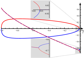
Figure 20: Eigenvalues of $\mathbf{M}\left(\gamma\right)$ (in units of $1/\sigma$) as a function of $\gamma$. Dashed lines: real part, solid lines: imaginary part.

Appendix F RG flow for externally screened interaction

If the single layer screening length $\kappa_{s}^{-1}$ and the typical length scale $L_{E}$ (e.g. the thermal length) exceed the distance to the electrostatic gates, the external screening of interactions can no longer be neglected. Effectively, the interactions become short ranged. This implies the breakdown of $\mathcal{F}$-invariance. As a consequence, the relations for NL$\sigma$M parameters $\det\left(\underline{z}+\underline{\Gamma}\right)=0$ and $(z_{1}+\Gamma_{11})/(z_{2}+\Gamma_{22})=1$ (derived in the case of long-range interaction in Sec. III.7.2 and Appendix C.4) are no longer true. Note that the invariance under renormalization of $\left(\underline{z}+\underline{\Gamma}\right)$ is not a consequence of $\mathcal{F}$-invariance and still holds.

Here we present general RG equations that allow us to describe the crossover between the cases of long-range Coulomb interaction and of no interaction:

$$\rule{0.0pt}{12.91663pt}\rule[-8.61108pt]{0.0pt}{0.0pt}\frac{d\sigma_{1}}{dy} =\frac{2}{\pi}\Biggl{[}\frac{1}{2}-f\left(\frac{\Gamma_{11}}{z_{1}}\right)$$

$$-\frac{\sigma_{1}^{2}\Gamma_{12}^{2}\sum\limits_{\varsigma=\pm}\varsigma f_{2}\left(\frac{\sigma_{1}}{z_{1}},\frac{\sigma_{1}}{z_{1}+\Gamma_{11}},d_{\varsigma}\right)}{2z_{1}\left(z_{1}+\Gamma_{11}\right)\det\left(\underline{z}+\underline{\Gamma}\right)\left(d_{-}-d_{+}\right)}\Biggr{]}$$ (209a)

$$\rule{0.0pt}{12.91663pt}\rule[-8.61108pt]{0.0pt}{0.0pt}\frac{d\sigma_{2}}{dy} =\frac{2}{\pi}\Biggl{[}\frac{1}{2}-f\left(\frac{\Gamma_{22}}{z_{2}}\right),$$

$$-\frac{\sigma_{2}^{2}\Gamma_{12}^{2}\sum\limits_{\varsigma=\pm}\varsigma f_{2}\left(\frac{\sigma_{2}}{z_{2}},\frac{\sigma_{2}}{z_{2}+\Gamma_{22}},d_{\varsigma}\right)}{2z_{2}\left(z_{2}+\Gamma_{22}\right)\det\left(\underline{z}+\underline{\Gamma}\right)\left(d_{-}-d_{+}\right)}\Biggr{]},$$ (209b)

$$\rule{0.0pt}{12.91663pt}\rule[-8.61108pt]{0.0pt}{0.0pt}\frac{dz_{1}}{dy} =-\frac{d\Gamma_{11}}{dy}=\frac{\Gamma_{11}}{\pi\sigma_{1}},$$ (209c)

$$\rule{0.0pt}{12.91663pt}\rule[-8.61108pt]{0.0pt}{0.0pt}\frac{dz_{2}}{dy} =-\frac{d\Gamma_{22}}{dy}=\frac{\Gamma_{22}}{\pi\sigma_{2}}.$$ (209d)

In contrast to the Coulomb case (Eq. (101)), these RG equations can not be expressed in terms of the parameter $\gamma_{ss}=\Gamma_{ss}/z_{s}$. Further, we emphasize that the RG equations for $\Gamma_{ss}$ and $z_{s}$ are exactly the same as in the Coulomb case. In particular, $\Gamma_{12}$ is not renormalized, since the general arguments exposed in Sec. IV.2 hold also in the case of short ranged interactions. It is worthwhile to repeat that $0\leq|\Gamma_{ss}|\leq z_{s}$ and typically $|\Gamma_{12}|\leq\max_{s=1,2}|\Gamma_{ss}|$.

For sufficiently strong interactions, the RG flow implies localizing behaviour of the conductivities. However, as the RG flow predicts decreasing interaction amplitudes, the system undergoes a crossover to the free-electron weak-antilocalization effect. (Note that also $\Gamma_{12}/z_{s}$ decreases.) Accordingly, similar to the case of Coulomb interaction, in the case of strong short range interactions we also predict a non-monotonic conductivity behaviour. The quantitative difference is the steeper antilocalizing slope in the final stage of the flow.

References

- Bernevig and Zhang (2006) B. A. Bernevig and S.-C. Zhang, Phys. Rev. Lett. 96, 106802 (2006).
- Bernevig et al. (2006) B. A. Bernevig, T. L. Hughes, and S.-C. Zhang, Science 314, 1757 (2006).
- Fu et al. (2007) L. Fu, C. L. Kane, and E. J. Mele, Phys. Rev. Lett. 98, 106803 (2007).
- Moore and Balents (2007) J. E. Moore and L. Balents, Phys. Rev. B 75, 121306 (2007).
- Roy (2009) R. Roy, Phys. Rev. B 79, 195322 (2009).
- König et al. (2007) M. König, S. Wiedmann, C. Brüne, A. Roth, H. Buhmann, L. W. Molenkamp, X.-L. Qi, and S.-C. Zhang, Science 318, 766 (2007).
- Hsieh et al. (2008) D. Hsieh, D. Qian, L. Wray, Y. Xia, Y. S. Hor, and M. Z. Cava, R. J. Hasan, Nature 452, 970 (2008).
- Hasan and Kane (2010) M. Z. Hasan and C. L. Kane, Rev. Mod. Phys. 82, 3045 (2010).
- Qi and Zhang (2011) X.-L. Qi and S.-C. Zhang, Rev. Mod. Phys. 83, 1057 (2011).
- Schnyder et al. (2008) A. P. Schnyder, S. Ryu, A. Furusaki, and A. W. W. Ludwig, Phys. Rev. B 78, 195125 (2008).
- Kitaev (2009) A. Kitaev, AIP Conference Proceedings 1134, 22 (2009).
- Gurarie (2011) V. Gurarie, Phys. Rev. B 83, 085426 (2011).
- Klitzing et al. (1980) K. v. Klitzing, G. Dorda, and M. Pepper, Phys. Rev. Lett. 45, 494 (1980).
- Thouless et al. (1982) D. J. Thouless, M. Kohmoto, M. P. Nightingale, and M. den Nijs, Phys. Rev. Lett. 49, 405 (1982).
- Culcer (2012) D. Culcer, Physica E 44, 860 (2012).
- (16) H. Steinberg, D. R. Gardner, Y. S. Lee, and P. Jarillo- Herrero, Nano Lett. 10, 5032 (2010).
- (17) J. G. Checkelsky, Y. S. Hor, R. J. Cava, N. P. Ong, Phys. Rev. Lett. 106, 196801 (2011).
- (18) D. Kim, S. Cho, N.P. Butch, P. Syers, K. Kirshenbaum, S. Adam, J. Paglione and M.S. Fuhrer, Nature Physics 8, 460-464 (2012).
- (19) S.S. Hong, J.J. Cha, D. Kong and Y. Cui, Nat. Comm. 3, 757 (2012).
- (20) D. Kim, Q. Li, P. Syers, N. P. Butch, J. Paglione, S. Das Sarma, and M. S. Fuhrer, Phys. Rev. Lett. 109, 166801 (2012).
- (21) P. Cheng, C. Song, T. Zhang, Y. Zhang, Y. Wang, J.-F. Jia, J. Wang, Y. Wang, B.-F. Zhu, X. Chen, et al., Phys. Rev. Lett. 105, 076801, (2010).
- (22) T. Hanaguri, K. Igarashi, M. Kawamura, H. Takagi, T. Sasagawa, Phys. Rev. B 82, 081305, (2010).
- (23) J. G. Analytis, R. D. McDonald, S. C. Riggs, J.-H. Chu, G. S. Boebinger, and I. R. Fisher, Nat. Phys. 6, 960 (2010).
- (24) B. Sacépé, J. B. Oostinga, J. Li, A. Ubaldini, N.J.G. Couto, E. Giannini, and A. F. Morpurgo, Nat. Comm. 2, 575 (2011).
- Brüne et al. (2011) C. Brüne, C. X. Liu, E. G. Novik, E. M. Hankiewicz, H. Buhmann, Y. L. Chen, X. L. Qi, Z. X. Shen, S. C. Zhang, and L. W. Molenkamp, Phys. Rev. Lett. 106, 126803 (2011).
- (26) H. Peng, K. Lai, D. Kong, S. Meister, Y. Chen, X.-L. Qi, S.-C. Zhang, Z.-X. Shen, and Yi Cui, Nature Materials 9, 225229 (2010).
- (27) F. Xiu, L. He, Y. Wang, L. Cheng, L.-T. Chang, M. Lang, G. Huang, X. Kou, Y. Zhou, X. Jiang, Z. Chen, J. Zou, A. Shailos, and K. L. Wang, Nat. Nanotechnol. 6, 216 (2011).
- (28) J. Dufouleur, L. Veyrat, A. Teichgraber, S. Neuhaus, C. Nowka, S. Hampel, J. Cayssol, J. Schumann, B. Eichler, O. G. Schmidt, B. Buchner, and R. Giraud, Phys. Rev. Lett. 110, 186806 (2013) .
- (29) H. Steinberg, J.B. Laloë, V. Fatemi, J.S. Moodera and P. Jarillo-Herrero, Phys. Rev. B 84, 233101 (2011).
- (30) G. Zhang, H. Qin, J. Chen, X. He, L. Lu, Y. Li and K. Wu, Adv. Func. Mater. 21, 2351 (2011).
- Chen et al. (2011) J. Chen, X. Y. He, K. H. Wu, Z. Q. Ji, L. Lu, J. R. Shi, J. H. Smet, and Y. Q. Li, Phys. Rev. B 83, 241304 (2011).
- (32) J. Wang, A. M. DaSilva, C.-Z. Chang, K. He, J. K. Jain, N. Samarth, X.-C. Ma, Q.-K. Xue, and Moses H. W. Chan, Phys. Rev. B 83, 245438 (2011).
- (33) M. Liu, C.-Z. Chang, Z. Zhang, Y. Zhang, W. Ruan, K. He, L.-L. Wang, X. Chen, J.-F. Jia, S.-C. Zhang, et al., Phys. Rev. B 83, 165440 (2011).
- Alt (1985) B. L. Altshuler and A. G. Aronov, in Electron-Electron Interactions in Disordered Conductors, edited by A. J. Efros and M. Pollack (North-Holland, Amsterdam, 1985).
- Ostrovsky et al. (2010) P. M. Ostrovsky, I. V. Gornyi, and A. D. Mirlin, Phys. Rev. Lett. 105, 036803 (2010).
- Burmistrov et al. (2011) I. S. Burmistrov, I. V. Gornyi, and K. S. Tikhonov, Phys. Rev. B 84, 075338 (2011).
- Minkov et al. (2011) G. M. Minkov, A. V. Germanenko, O. E. Rut, A. A. Sherstobitov, A. K. Bakarov, and D. V. Dmitriev, Phys. Rev. B 84, 075337 (2011).
- A.M.Finkel’stein (1983) A.M.Finkel’stein, Zh. Eksp. Teor. Fiz. 84, 168 (1983).
- A.M.Finkel’stein (1984) A.M.Finkel’stein, Z. Phys. B: Con. Mat. 56, 189 (1984).
- Finkelstein (1990) A. M. Finkelstein, in Soviet scientific reviews: Physics reviews, edited by I. M. Khalatnikov (Harwood Academic Publishers, 1990), vol. 14, p. 1.
- Belitz and Kirkpatrick (1994) D. Belitz and T. R. Kirkpatrick, Rev. Mod. Phys. 66, 261 (1994).
- Finkel’stein (2010) A. M. Finkel’stein, in 50 years of Anderson Localization, edited by E. Abrahams (World scientific, 2010), p. 385.
- Castellani et al. (1984) C. Castellani, C. Di Castro, P. A. Lee, and M. Ma, Phys. Rev. B 30, 527 (1984).
- Finkel’stein (1987) A. Finkel’stein, Pis’ma v ZhETF 45 (1), 37 (1987), [A.M. Finkel’stein, JETP Lett. 45 (1), 46-49 (1987)].
- Finkel’stein (1994) A. Finkel’stein, Physica B 197, 636 (1994).
- A.M.M. Pruisken (1995) M. B. A.M.M. Pruisken, EuroPhys. Lett. 31, 543 (1995).
- Pruisken and Burmistrov (2007) A. Pruisken and I. Burmistrov, Annals of Physics 322, 1265 (2007).
- Punnoose and Finkel’stein (2005) A. Punnoose and A. M. Finkel’stein, Science 310, 289 (2005).
- Zheng and MacDonald (1993) L. Zheng and A. H. MacDonald, Phys. Rev. B 48, 8203 (1993).
- Kamenev and Oreg (1995) A. Kamenev and Y. Oreg, Phys. Rev. B 52, 7516 (1995).
- Flensberg et al. (1995) K. Flensberg, B. Y.-K. Hu, A.-P. Jauho, and J. M. Kinaret, Phys. Rev. B 52, 14761 (1995).
- Linder et al. (2009) J. Linder, T. Yokoyama, and A. Sudbø, Phys. Rev. B 80, 205401 (2009).
- Taskin et al. (2012) A. A. Taskin, S. Sasaki, K. Segawa, and Y. Ando, Phys. Rev. Lett. 109, 066803 (2012).
- (54) R. E. V. Profumo, M. Polini, R. Asgari, R. Fazio, and A. H. MacDonald, Phys. Rev. B 82, 085443, (2010).
- (55) M. I. Katsnelson, Phys. Rev. B 84, 041407(R) (2011).
- Carrega et al. (2012) M. Carrega, T. Tudorovskiy, A. Principi, M. I. Katsnelson, and M. Polini, New J. Phys. 14, 063033 (2012).
- Zhang et al. (2012) F. Zhang, C. L. Kane, and E. J. Mele, Phys. Rev. B 86, 081303 (2012).
- González et al. (2001) J. González, F. Guinea, and M. A. H. Vozmediano, Phys. Rev. B 63, 134421 (2001).
- Foster and Aleiner (2008) M. S. Foster and I. L. Aleiner, Phys. Rev. B 77, 195413 (2008).
- Sheehy and Schmalian (2007) D. E. Sheehy and J. Schmalian, Phys. Rev. Lett. 99, 226803 (2007).
- Aleiner and Efetov (2006) I. L. Aleiner and K. B. Efetov, Phys. Rev. Lett. 97, 236801 (2006).
- Ostrovsky et al. (2006) P. M. Ostrovsky, I. V. Gornyi, and A. D. Mirlin, Phys. Rev. B 74, 235443 (2006).
- Schuessler et al. (2009) A. Schuessler, P. M. Ostrovsky, I. V. Gornyi, and A. D. Mirlin, Phys. Rev. B 79, 075405 (2009).
- Adroguer et al. (2012) P. Adroguer, D. Carpentier, J. Cayssol, and E. Orignac, New J. Phys. 14, 103027 (2012).
- (65) M. Sitte, A. Rosch, and L. Fritz (2013), arXiv:1305.1788.
- Peres et al. (2005) N. M. R. Peres, F. Guinea, and A. H. Castro Neto, Phys. Rev. B 72, 174406 (2005).
- Seradjeh et al. (2009) B. Seradjeh, J. E. Moore, and M. Franz, Phys. Rev. Lett. 103, 066402 (2009).
- Pruisken et al. (1999) A. M. M. Pruisken, M. A. Baranov, and B. Skoric, Phys. Rev. B 60, 16807 (1999).
- Efe (1980) K. B. Efetov, A. I. Larkin, and D. E. Khmel’nitskii, Sov. Phys. JETP 52(3), 568 (1980).
- Witten (1984) E. Witten, Commun. Math. Phys. 92, 455 (1984).
- Nersesyan et al. (1994) A. A. Nersesyan, A. M. Tsvelik, and F. Wenger, Phys. Rev. Lett. 72, 2628 (1994).
- Nersesyan et al. (1995) A. Nersesyan, A. Tsvelik, and F. Wenger, Nucl. Phys. B 438, 561 (1995).
- Altland et al. (2002) A. Altland, B. Simons, and M. Zirnbauer, Phys. Rep. 359, 283 (2002).
- Altland (2006) A. Altland, Phys. Rev. Lett. 97, 236802 (2006).
- König et al. (2012) E. J. König, P. M. Ostrovsky, I. V. Protopopov, and A. D. Mirlin, Phys. Rev. B 85, 195130 (2012).
- Ryu et al. (2007) S. Ryu, C. Mudry, H. Obuse, and A. Furusaki, Phys. Rev. Lett. 99, 116601 (2007).
- Ostrovsky et al. (2007) P. M. Ostrovsky, I. V. Gornyi, and A. D. Mirlin, Phys. Rev. Lett. 98, 256801 (2007).
- Fu and Kane (2012) L. Fu and C. L. Kane, Phys. Rev. Lett. 109, 246605 (2012).
- Nozieres and Luttinger (1962) P. Nozieres and J. Luttinger, Phys. Rev. 127, 1423 (1962).
- Abrikosov et al. (1963) A. A. Abrikosov, L. P. Gorkov, and I. E. Dzyaloshinskij, Methods of quantum field theory in statistical physics (Prentice-Hall, Englewood Cliffs, NJ, 1963).
- Lifshitz et al. (1980) E. M. Lifshitz, and L. P. Pitaevskij, Course of theoretical physics, vol. 9: Statistical physics, part 2: theory of condensed state (1980).
- (82) R. Nandkishore, J. Maciejko, D. A. Huse, and S. L. Sondhi, Phys. Rev. B 87, 174511 (2013).
- Burmistrov et al. (2012) I. S. Burmistrov, I. V. Gornyi, and A. D. Mirlin, Phys. Rev. Lett. 108, 017002 (2012).
- Polyakov and Wiegmann (1983) A. Polyakov and P. Wiegmann, Phys. Lett. B 131, 121 (1983).
- Vecchia et al. (1984) P. D. Vecchia, B. Durhuus, and J. Petersen, Phys. Lett. B 144, 245 (1984).
- Faddeev (1976) L. Faddeev, Lett. Math. Phys. 1, 289 (1976).
- Gerasimov (1993) A. Gerasimov (1993), eprint arXiv:hep-th/9305090.
- Losev et al. (1995) A. Losev, G. Moore, N. Nekrasov, and S. Shatashvili (1995), eprint arXiv:hep-th/9511185v2.
- Smilga (1996) A. V. Smilga, Phys. Rev. D 54, 7757 (1996).
- Nomura et al. (2008) K. Nomura, S. Ryu, M. Koshino, C. Mudry, and A. Furusaki, Phys. Rev. Lett. 100, 246806 (2008).
- Qi et al. (2008) X.-L. Qi, T. L. Hughes, and S.-C. Zhang, Phys. Rev. B 78, 195424 (2008).
- Qi et al. (2009) X.-L. Qi, R. Li, J. Zang, and S.-C. Zhang, Science 323, 1184 (2009).
- Essin et al. (2009) A. M. Essin, J. E. Moore, and D. Vanderbilt, Phys. Rev. Lett. 102, 146805 (2009).
- Pesin and MacDonald (2012) D. A. Pesin and A. H. MacDonald (2012), eprint arXiv:1207.4444v1.
- Ostrovsky et al. (2008) P. M. Ostrovsky, I. V. Gornyi, and A. D. Mirlin, Phys. Rev. B 77, 195430 (2008).
- Pruisken (1990) A. M. M. Pruisken, in The Quantum Hall Effect, edited by R. E. Prange and S. M. Girvin (Springer-Verlag, Berlin, 1990).
- Pruisken and Burmistrov (2005) A. Pruisken and I. Burmistrov, Annals of Physics 316, 285 (2005).
- Bocquet et al. (2000) M. Bocquet, D. Serban, and M. Zirnbauer, Nucl. Phys. B 578, 628 (2000).
- Baranov et al. (1999) M. A. Baranov, A. M. M. Pruisken, and B. Skorić, Phys. Rev. B 60, 16821 (1999).
- Hikami et al. (1980) S. Hikami, A. I. Larkin, and Y. Nagaoka, Progress of Theoretical Physics 63, 707 (1980).
- Castellani and Di Castro (1986) C. Castellani and C. Di Castro, Phys. Rev. B 34, 5935 (1986).
- (102) T. Ohtsuki, K. Slevin, B. Kramer, Physica E 22, 248 (2004).
- Markos and Schweitzer (2006) P. Markos and L. Schweitzer, J. Phys. A - Math. Gen. 39, 3221 (2006).
- (104) F. Evers and A. D. Mirlin, Rev. Mod. Phys. 80, 1355 (2008).
- Bardarson et al. (2007) J. H. Bardarson, J. Tworzydło, P. W. Brouwer, and C. W. J. Beenakker, Phys. Rev. Lett. 99, 106801 (2007).
- Nomura et al. (2007) K. Nomura, M. Koshino, and S. Ryu, Phys. Rev. Lett. 99, 146806 (2007).
- Ostrovsky et al. (2012) P. M. Ostrovsky, I. V. Gornyi, and A. D. Mirlin, Phys. Rev. B 86, 125323 (2012).
- Garate and Glazman (2012) I. Garate and L. Glazman, Phys. Rev. B 86, 035422 (2012).
- Krueckl and Richter (2012) V. Krueckl and K. Richter, Semicond. Sci. Tech. 27, 124006 (2012).
- Li (2012) Y. Li (2012), private communication.
- (111) J. Baars, F. Sorger, Solid State Commun. 10, 875 (1972).
- Hancock et al. (2011) J. N. Hancock, J. L. M. van Mechelen, A. B. Kuzmenko, D. van der Marel, C. Brüne, E. G. Novik, G. V. Astakhov, H. Buhmann, and L. W. Molenkamp, Phys. Rev. Lett. 107, 136803 (2011).
- Ringel et al. (2012) Z. Ringel, Y. E. Kraus, and A. Stern, Phys. Rev. B 86, 045102 (2012).
- (114) K. Kobayashi, T. Ohtsuki, K.-I. Imura (2013), arXiv:1210.4656v2 (accepted for Phys. Rev. Lett. on 05/17/2013).
- Solomon et al. (1989) P. M. Solomon, P. J. Price, D. J. Frank, and D. C. La Tulipe, Phys. Rev. Lett. 63, 2508 (1989).
- Gramila et al. (1991) T. J. Gramila, J. P. Eisenstein, A. H. MacDonald, L. N. Pfeiffer, and K. W. West, Phys. Rev. Lett. 66, 1216 (1991).
- Schütt et al. (2013) M. Schütt, P. M. Ostrovsky, M. Titov, I. V. Gornyi, B. N. Narozhny, and A. D. Mirlin, Phys. Rev. Lett. 110, 026601 (2013).
- Wray et al. (2010) L. A. Wray, S. Xu, Y. Xia, D. Qian, A. V. Fedorov, H. Lin, A. Bansil, Y. S. Hor, R. J. Cava, and M. Z. Hasan, Nat. Phys. 6, 855 (2010).
- (119) Related problem on interaction effects on the surface of 3D topological superconductor of class CI was studied in M. S. Foster, E. A. Yuzbashyan, Phys. Rev. Lett. 109, 246801 (2012).
- Zhang et al. (2010) W. Zhang, R. Yu, H.-J. Zhang, X. Dai, and Z. Fang, New J. Phys. 12, 065013 (2010).