Discussion on common errors in analyzing sea level accelerations, solar trends and global warming

Zusammenfassung

Herein I discuss common errors in applying regression models and wavelet filters used to analyze geophysical signals. I demonstrate that: (1) multidecadal natural oscillations (e.g. the quasi 60 yr Multidecadal Atlantic Oscillation (AMO), North Atlantic Oscillation (NAO) and Pacific Decadal Oscillation (PDO)) need to be taken into account for properly quantifying anomalous background accelerations in tide gauge records such as in New York City; (2) uncertainties and multicollinearity among climate forcing functions also prevent a proper evaluation of the solar contribution to the 20th century global surface temperature warming using overloaded linear regression models during the 1900–2000 period alone; (3) when periodic wavelet filters, which require that a record is pre-processed with a reflection methodology, are improperly applied to decompose non-stationary solar and climatic time series, Gibbs boundary artifacts emerge yielding misleading physical interpretations. By correcting these errors and using optimized regression models that reduce multicollinearity artifacts, I found the following results: (1) the relative sea level in New York City is not accelerating in an alarming way, and may increase by about $350\pm 30$ mm from 2000 to 2100 instead of the previously projected values varying from $1130\pm 480$ mm to $1550\pm 400$ mm estimated using the methods proposed, e.g., by Sallenger Jr. et al. (2012) and Boon (2012), respectively; (2) the solar activity increase during the 20th century contributed at least about 50 % of the 0.8 ^∘C global warming observed during the 20th century instead of only 7–10 % (e.g.: IPCC, 2007; Benestad and Schmidt, 2009; Lean and Rind, 2009; Rohde et al., 2013). The first result was obtained by using a quadratic polynomial function plus a 60 yr harmonic to fit a required 110 yr-long sea level record. The second result was obtained by using solar, volcano, greenhouse gases and aerosol constructors to fit modern paleoclimatic temperature reconstructions (e.g.: Moberg et al., 2005; Mann et al., 2008; Christiansen and Ljungqvist, 2012) since the Medieval Warm Period, which show a large millennial cycle that is well correlated to the millennial solar cycle (e.g.: Kirkby, 2007; Scafetta and West, 2007; Scafetta, 2012c). These findings stress the importance of natural oscillations and of the sun to properly interpret climatic changes.

$\sim$

Cite this article as: Scafetta, N.: Common errors in analyzing sea level accelerations, solar trends and temperature records. Pattern Recognition in Physics 1, 37-58, doi: 10.5194/prp-1-37-2013, 2013.

Geophysical systems are usually studied by analyzing time series. The purpose of the analysis is to recognize specific physical patterns and to provide appropriate physical interpretations. Improper applications of complex mathematical and statistical methodologies are possible, and can yield erroneous interpretations. Addressing this issue is important because errors present in the scientific literature may not be promptly recognized and, therefore, may propagate misleading scientists and policymakers and, eventually, delay scientific progress.

Herein I briefly discuss a few important examples found in the geophysical literature where time series tools of analysis were misapplied. These cases mostly involve multicollinearity artifacts in linear regression models and Gibbs artifacts in wavelet filters. The following examples are studied: (1) the necessity of recognizing and taking into account multidecadal natural oscillations for properly quantifying anomalous accelerations in tide gauge records; (2) the risk of improperly using overloaded multilinear regression models to interpret global surface temperature records; (3) how to recognize Gibbs boundary artifacts that can emerge when periodic wavelet filters are improperly applied to decompose non-stationary geophysical time series. The proposed reanalyses correct a number of erroneous interpretations while stressing the importance of natural oscillations and of the sun to properly interpret climatic changes.

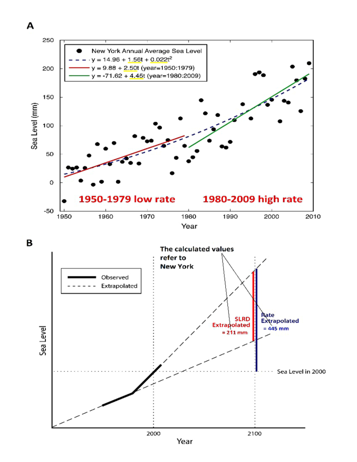
Abbildung 1: Reproduction and comments of Sallenger Jr. et al. (2012)’s figures S7 and S8. (A) Sea level record in New York as interpreted in Sallenger Jr. et al. (2012)’s figures S7 in their supplementary file. (B) Predicted sea level rate difference between the two half-window series (SLRD) for the 21st century as interpreted in Sallenger Jr. et al. (2012)’s figures S8 in their supplementary file.

1 Sea level accelerations versus 60-year oscillations: the New York City case

Tide gauge records are characterized by complex dynamics driven by different forces that on multidecadal and multisecular scales are regulated by a combination of ocean dynamics, of eustasy, isostasy and subsidence mechanisms, and of global warming (Boon, 2012; Jevrejeva et al., 2008; Mörner, 2010, 2013; Sallenger Jr. et al., 2012). Understanding these dynamics and correctly quantifying accelerations in tide gauge records is important for numerous civil purposes. However, changes of rate due to specific multidecadal natural oscillations should be recognized and separated from a background acceleration that may be potentially induced by alternative factors such as anthropogenic global warming. Let us discuss an important example where this physical aspect was apparently not properly recognized by Sallenger Jr. et al. (2012) and Boon (2012).

Figure 1a and b reproduce (with a few additional comments) figures S7 and S8 of the supplementary information file published in Sallenger Jr. et al. (2012), indicated herein as Sa2012. Sa2012’s method for interpreting tide gauge records is detailed below. The example uses the New York City (NYC) (the Battery) annual average tide gauge record that can be downloaded from the Permanent Service for Mean Sea Level (PSMSL) (http://www.psmsl.org/) (Woodworth and Player, 2003).

As Fig. 1a shows, Sa2012 analyzed the tide gauge record for NYC from 1950 to 2009; note, however, that Sa2012’s choice appears already surprising because these data have been available since 1856. Sa2012 linearly fit the periods 1950–1979 and 1980–2009, and found that during 1950–1979 the sea level rose with a rate of $2.5\pm 0.6$ mm yr^-1, while during 1980–2009 the rate increased to $4.45\pm 0.72$ mm yr^-1. Thus, a strong apparent acceleration was discovered and was interpreted as due to the anthropogenic warming of the last 40 yr, which could have caused a significant change in the strength of the Atlantic Meridional overturning circulation and of the Gulf Stream. This acceleration was more conveniently calculated by fitting the 1950–2009 period with a second order polynomial, e.g.:

$$g(t)=\frac{1}{2}a(t-2000)^{2}+v(t-2000)+c.$$ (1)

For NYC a 1950–2009 acceleration of $a=0.044\pm 0.030$ mm yr^-2 was found. Then, Sa2012 repeated the quadratic fit to evaluate the acceleration during the periods 1960–2009 and 1970–2009, and for NYC the results would be $a=0.083\pm 0.049$ mm yr^-2 and $a=0.133\pm 0.093$ mm yr^-2, respectively. Similarly, Boon (2012) fit the period from 1969 to 2011 and found $a=0.20\pm 0.07$ mm yr^-2.

Thus, in NYC not only would the sea level be alarmingly accelerating, but the acceleration itself has also incrementally increased during the last decades. Similar results were claimed for other Atlantic coast cities of North America. Finally, as shown in Fig. 1b, Sa2012 extrapolated its fit curves to 2100 and calculated the sea level rate difference (SLRD) to provide a first approximation estimate of the anthropogenic global warming effect on the sea level rise during the 21st century. For NYC, SLRD would be $\sim 211$ mm if the 1950–1979 and 1980–2009 linear extrapolated trends (reported in the insert of Fig. 1a) were used, but SLRD would increase to about $\sim 890$ mm if the 1950–1979 linear trend was compared against the 1970–2009 quadratic polynomial fit extrapolation. Alternatively, by also taking into account the statistical uncertainty in the regression coefficients, NYC might experience a net sea level rise of $\sim 1130\pm 480$ mm from 2000 to 2100 if Eq. (1) is used to fit the 1970–2009 period ($a=0.133\pm 0.093$ mm yr^-2, $v=4.6\pm 1.1$ mm yr^-1, $c=7084\pm 8$ mm) and extrapolated to 2100.

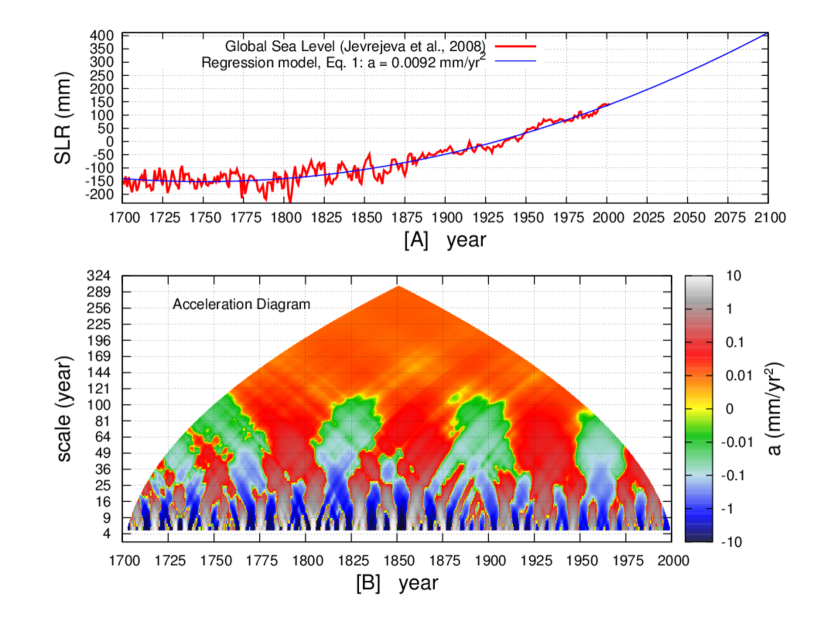
Abbildung 2: (A) Estimate of the global sea level rise (Jevrejeva et al., 2008) fit with Eq. (1) (blue). (B) Scale-by-scale acceleration diagram of (B) demonstrating large quasi 60–70 yr oscillations manifested by the alternating positive (red area) and negative (green area) accelerations at scales up to 110 yr.

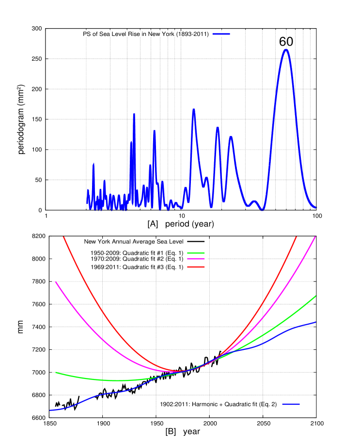
Abbildung 3: (A) Periodogram of the tide gauge record for New York City (1893–2011) that highlights a dominant quasi 60 yr oscillation. The data are linearly detrended before applying the periodogram algorithm for improved stability at lower frequencies. (B) Sea level record for New York City (black) fitted with Eq. (2) (blue) from 1902 to 2011, and with the Eq. (1) from 1950 to 2009 (green), from 1970 to 2009 (purple) and from 1969 to 2011 (red). Projections #1 and #2 use Sallenger Jr. et al. (2012)’s method, projection #3 uses Boon’s (2012) method. The blue model agrees far better with the data since 1856 and likely produces the most realistic projection for the 21st century; see also Scafetta (2013) for additional details.

However, Sa2012’s result does not appear robust because, as I will demonstrate below, the geometrical convexity observed in the NYC tide gauge record from 1950 to 2009 was very likely mostly induced by a quasi 60 yr oscillation that is already known to exist in the climate system. In fact, numerous ocean indexes such as the Multidecadal Atlantic Oscillation (AMO), the North Atlantic Oscillation (NAO) and the Pacific Decadal Oscillation (PDO) oscillate with a quasi 60 yr period for centuries and millennia (e.g.: Mörner, 1989, 1990; Klyashtorin et al., 2009; Mazzarella and Scafetta, 2012; Knudsen et al., 2011; Scafetta, 2013), as well as global surface temperature records (e.g.: Kobashi et al., 2010; Qian and Lu, 2010; Scafetta, 2010, 2012a; Schulz and Paul, 2002). In particular, Scafetta (2010, 2012c, 2012d) provided empirical and theoretical evidence that the observed multidecadal oscillation could be solar/astronomical-induced, could be about 60 yr-long from 1850 to 2012 and could be modulated by other quasi-secular oscillations (e.g.: Ogurtsov et al., 2002; Scafetta, 2012c; Scafetta and Willson, 2013). In fact, a quasi 60 yr oscillation is particularly evident in the global temperature records since 1850: 1850–1880, 1910–1940 and 1970–2000 were warming periods and 1880–1910, 1940–1970 and 2000–(2030?) were cooling periods. This quasi 60 yr oscillation is superposed to a background warming trend which may be due to multiple causes (e.g.: solar activity, anthropogenic forcings and urban heat island effects) (e.g.: Scafetta and West, 2007; Scafetta, 2009, 2010, 2012a, 2012b, 2012c). Because the climate system is evidently characterized by numerous oscillations, tide gauge records could be characterized by equivalent oscillations too.

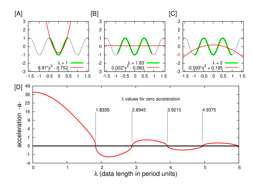
Abbildung 4: (A), (B) and (C) show a stationary harmonic signal (black) of unit period fit with Eq. (1) (red) using three different records length (green), $\lambda=1$, $1.83$ and $2$, respectively. (D) The regression acceleration coefficient in function of the record length $\lambda$. The figure highlights the values of $\lambda$ that make the acceleration $a=0$, indicating regression orthogonality between the harmonic signal and the quadratic polynomial. From Scafetta (2013).

Indeed, a quasi 60 yr oscillation has been found in numerous sea level records since 1700 (Chambers et al., 2012; Jevrejeva et al., 2008; Parker, 2013). Figure 2a shows the global sea level record from 1700 to 2000 proposed by Jevrejeva et al. (2008) fit with Eq. (1) ($a=0.0092\pm 0.0004$ mm yr^-2; $v=2.31\pm 0.06$ mm yr^-1; $c=136\pm 4$ mm). In addition to a relatively small acceleration since 1700 AD, which, if continues, will cause a global sea level rise of about $277\pm 8$ mm from 2000 to 2100, the global sea level record clearly presents large 60–70 yr oscillations. This is better demonstrated in Fig. 2b that shows the scale-by-scale palette acceleration diagram of this global sea level record (Jevrejeva et al., 2008; Scafetta, 2013). Here the color of a dot at coordinate (x, y) indicates the acceleration $a$ (calculated with Eq.  1) of a $y$-year-long interval centered in $x$. The color of the dot at the top of the diagram, which in this case is approximately orange, indicates the global acceleration for the 1700–2000 period, $a=0.0092\pm 0.0004$ mm yr^-2. The diagram also suggests that for scales larger than 110 yr the acceleration is almost homogeneous, around $0.01$ mm yr^-2 or less (orange/yellow color) at all scales and times (Scafetta, 2013). For example, during the preindustrial 1700–1900 period $a=0.009\pm 0.001$ mm yr^-2; during the industrial 1900–2000 period $a=0.010\pm 0.0004$ mm yr^-2. Thus, the observed acceleration appears to be independent of the 20th century anthropogenic global warming and could be a consequence of other phenomena, such as the quasi-millennial solar/climate cycle (Bond et al., 2001; Kerr, 2001; Kobashi et al., 2013; Kirkby, 2007; Scafetta, 2012c) observed throughout the Holocene. The millennial solar/climatic cycle has been in its warming phase since 1700, which characterized the Maunder solar minimum during the Little Ice Age. Finally, the alternating quasi regular large green and red areas evident at scales from 30 to 110 yr indicate a change of acceleration (from negative to positive, and vice-versa) that reveals the existence of a quasi 60–70 yr oscillation since 1700. Strong quasi decadal and bidecadal oscillations are observed at scales below 30 yr. In conclusion, because the global sea level record presents a clear quasi 60 yr oscillation that also well correlates with the quasi 60 yr oscillation found in the NAO index since 1700 (Scafetta, 2013), there is the need to check whether the tide gauge record of NYC too may have been affected by a quasi 60 yr oscillation.

Herein I extend the finding discussed in Scafetta (2013). Figure 3a shows the periodogram of the tide gauge record for NYC from 1893 to 2011: the data available before 1893 are excluded from the analysis because the record is seriously incomplete. The periodogram is calculated after the three missing years (in 1992, 1994 and 2001) are linearly interpolated, and the linear trend ($y(t)=2.98(t-2000)+7088$) is detrended because the periodogram gives optimal results if the time series is stationary. The spectral analysis clearly highlights, among other minor spectral peaks, a dominant frequency at a period of about 60 yr, which is a typical major multidecadal oscillation found in PDO, AMO and NAO indexes (Klyashtorin et al., 2009; Knudsen et al., 2011; Mazzarella and Scafetta, 2012; Scafetta, 2012a, 2013; Manzi et al., 2012). This quasi 60 yr oscillation, after all, is clearly visible in the NYC tide gauge record once this record is plotted since 1856, as shown in Fig. 3b.

Consequently, for detecting a possible background sea level acceleration for NYC there is a need of adopting an upgraded regression model that at least must be made of a harmonic component plus a quadratic function of the type:

$$f(t)=H\cos\left(2\pi\frac{t-T}{60}\right)+\frac{1}{2}a(t-2000)^{2}+v(t-2000)+c.$$ (2)

Other longer multisecular and millennial oscillations may be added to the model (Bond et al., 2001; Kerr, 2001; Ogurtsov et al., 2002; Qian and Lu, 2010; Scafetta, 2012c; Schulz and Paul, 2002) but, because only about one century of data are herein analyzed, Eq. (2) cannot be expanded.

To determine the exact length of the time period required to avoid multicollinearity and make the 60 yr oscillation orthogonal to the quadratic polynomial term, a test proposed in Scafetta (2013) is herein rediscussed for the benefit of the reader. Figure 4a, b and c show fits of a periodic signal of unit period 1 of different length with a quadratic polynomial: the acceleration clearly varies in function of the length of the record $\lambda$. Figure 4d shows that the acceleration $a$ oscillates around zero in function of $\lambda$. The minimum length that makes the acceleration zero is $\lambda=1.8335$ times the length of the period of the oscillation. Thus, to optimally separate a 60 yr oscillation from a background acceleration, there is the need of using a $1.8335\times 60=110$ yr-long sequence. Indeed, as Fig. 2b shows, the alternation between the red and the green areas ends at scales close to $110$ yr indicating that there is the need of using more than 100 yr for filtering a background acceleration out from the quasi 60 yr oscillation.

Note that Sa2012’s regression model was applied to 60 yr-long and shorter intervals from 1950 to 2009. As Fig. 4a and d clearly show, using 60 yr-long and shorter records ($\lambda\leq 1$ period of the oscillation), makes the regression model unable to separate a background acceleration from a 60 yr oscillation because the two curves are significantly collinear, and a strong acceleration simply related to the bending of the 60 yr oscillation would be found. In the next section, the multicollinearity problem in regression models will be discussed more extensively.

NYC sea level data have been intermittently available since 1856, but as of 1893 only three annual means are missing, so the model given by Eq. (2) can be tested for this record because it is about 120 yr long from 1893 to 2011. Figure 3b shows the sea level record for NYC since 1856 (black) fitted with Eq. (2) for the required optimal 110 yr interval from 1902 to 2011 (blue). The fit gives $H=16\pm 4$ mm; $T=1956\pm 2.5$ yr; $a=0.006\pm 0.005$ mm yr^-2; $v=3.3\pm 0.3$ mm yr^-1; $c=7094\pm 6$ mm. For comparison, Fig. 3b also shows Sa2012’s and Boon’s (2012) methods using Eq. (1): (1) the fit is done from 1950 to 2009 (green) ($a=0.044\pm 0.030$ mm yr^-2, $v=3.7\pm 0.7$ mm yr^-1, $c=7086\pm 7$ mm); (2) the fit is done from 1970 to 2009 (purple) ($a=0.133\pm 0.1$ mm yr^-2, $v=4.6\pm 1.1$ mm yr^-1, $c=7084\pm 8$ mm); (3) the fit is done from 1969 to 2011 (red) ($a=0.20\pm 0.07$ mm yr^-2, $v=5.5\pm 0.9$ mm yr^-1, $c=7087\pm 7$ mm). Projections #1 and #2 use Sa2012’s method, projection #3 uses Boon’s (2012) method.

To test the sufficient stability of my result, the analysis for the two non-overlapping periods 1856–1934 and 1934–2012 is repeated. In the first case the fit gives $H=14\pm 6$ mm; $T=1963\pm 5$ yr; $a=0.018\pm 0.023$ mm yr^-2; $v=4.1\pm 2.4$ mm yr^-1; $c=7107\pm 122$ mm. In the second case the fit gives $H=16\pm 5$ mm; $T=1957\pm 5$ yr; $a=0.015\pm 0.027$ mm yr^-2; $v=3.6\pm 0.8$ mm yr^-1; $c=7095\pm 7$ mm. Because in the three cases the correspondent regression values are compatible to each other within their uncertainty and the regression model calibrated from 1856 to 1934 hindcasts the data from 1934 to 2012, and vice versa, the regression model, Eq. (2), can be considered sufficiently stable for interpreting the available data.

On the contrary, using Eq. (1) to fit 60 yr periods it is obtained: (1) from 1890 to 1949, $a=0.091\pm 0.027$ mm yr^-2; (2) from 1920 to 1979, $a=-0.043\pm 0.025$ mm yr^-2; (3) from 1950 to 2009, $a=0.044\pm 0.030$ mm yr^-2. Because the acceleration values of the three 60 yr sub-periods are not compatible to each other within their uncertainty, the regression model Eq. (1) does not capture the dynamics of the available NYC sea level data. However, the absolute values of the three accelerations are compatible to each other. Thus, the 1950–2009 acceleration value, $a=0.044\pm 0.03$ mm yr^-2, does not appear to be anomalous, but it is well within the natural variability of a system that oscillates with a quasi 60 yr cycle around a quasi linear upward trend. See Scafetta (2013) for additional discussion demonstrating that the accelerations found using the intervals proposed by Sa2012 and Boon (2012) are arbitrary.

Figure 3b also highlights that Eq. (2) hindcasts quite well the relative sea level in NYC from 1856 to 1901, whose period was not used to calibrate the regression model, which adopted only data from 1902 to 2011. Therefore, the model proposed in Eq. (2) reconstructs the available data since 1856, takes into account an influence of known climatic oscillations (e.g. the quasi 60 yr AMO oscillation) and may be reasonably used as a first approximation forecast tool. On the contrary, Sa2012 and Boon’s (2012) models immediately miss the data before 1950, 1969 and 1970, respectively, and ignore the existence of known multidecadal natural oscillations of the climate system. Consequently, the usefulness of the latter models for hindcast/forecast purposes should be questioned even on short periods. Essentially, Sa2012 Boon’s (2012) methodologies are too simplistic because, as evident in Fig. 3b, they do not capture the dynamics of the available data and, consequently, miss the true dynamical properties of the system.

As Fig. 3b shows, the adoption of Eq. (2) implies that the relative sea level in NYC accelerated 7 to 22 times less than what was obtained with Sa2012’s quadratic fit alone during the two 30 yr periods 1950–2009 and 1970–2009, respectively. By using the same extrapolation methodology proposed in Sa2012 and assuming that Eq. (2) persists during the 21st century, the relative sea level in NYC could rise about $350\pm 30$ mm from 2000 to 2100, which is significantly less than what Sa2012’s quadratic model extrapolation would suggest, that is up to about $1130\pm 480$ mm, or, using Boon’s (2012) model, the projected sea level would be $1550\pm 400$ mm from 2000 to 2100, as Fig. 3b shows.

In conclusion, the convexity of the NYC tide gauge record from 1950 to 2009 was very likely mostly induced by the quasi 60 yr AMO-NAO oscillation that strongly influences the Atlantic cost of North America and can be observed also in the global sea level record since 1700, shown in Fig. 2. However, Sa2012 mistook the 1950–2009 geometrical convexity of the NYC record as if it were due to an anomalous acceleration. Evidently, Sa2012’s 21st century projections for sea level rise in numerous locations need to be revised downward by taking it into account that the known multidecadal variability of the climate system would imply a significantly lower background acceleration than what they have estimated. A similar critique applies to the results by Boon (2012) too, who also used Eq. (1) to analyze a number of US and Canadian tide gauge records over a 43 yr period from 1969 to 2011 and, for NYC, he found a 1969–2011 acceleration of $a=0.20\pm 0.07$ mm yr^-2 and projected an alarming sea level rise of $570\pm 180$ mm above the 1983–2001 sea level mean by 2050. On the contrary, other authors (Houston and Dean, 2011; Parker, 2013; Scafetta, 2013) analyzed numerous secular-long tide gauge records and found small (positive or negative) accelerations close to zero ($\sim\pm 0.01$ mm yr^-2). Figure 2a shows that a global estimate of the sea level rise since 1700 presents an acceleration slightly smaller than $0.01$ mm yr^-2 since 1700, which may have also been partially driven by the great millennial solar/climate cycle (Bond et al., 2001; Kerr, 2001; Kirkby, 2007; Scafetta, 2012c), which will be more extensively discussed in the next section.

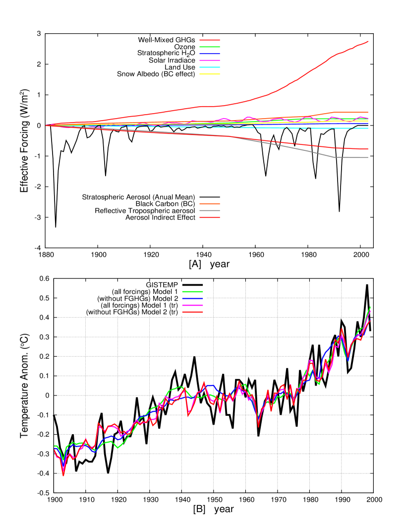
Abbildung 5: (A) The ten regression constructors used in Eq. (3) by Benestad and Schmidt (2009). (B) Four regression models of the global surface temperature record (GISTEMP) using all ten constructors (Model 1), and using nine constructors excluding the well-mixed greenhouse gases (CO₂ and CH₄) (Model 2). The two curves with -tr- adopt forcing functions truncated to the second decimal digit. See Table 2 for the regression coefficients.

2 Multi-linear regression models and the multicollinearity problem: estimates of the solar signature on climatic records

A number of authors have studied global surface temperature records using multilinear regression models to identify the relative contribution of known forcings of the earth’s temperature field. For example, Douglass and Clader (2002), and Gleisner and Thejll (2003) interpreted temperature records for the period 1980–2002 using four regression analysis constructors: an 11 yr solar cycle signal without any trend, the volcano signal, the ENSO signal, which captures fast climatic fluctuations, and a linear trend that can capture everything else responsible for the 1980–2002 warming trend, including the warming component induced by anthropogenic greenhouse gases (GHG). The four chosen constructors are sufficiently geometrically orthogonal and physically independent of each other. Geometrical orthogonality and physical independence are necessary conditions for efficiently decomposing a signal using multilinear regression models. On the contrary, multilinear regression models may produce seriously misleading and inconclusive results if used with constructors multicollinear to each other. In fact, it is well known that in presence of multicollinearity among the regression predictors the estimated regression coefficients may change quite erratically in response to even minor changes in the model or the data yielding misleading interpretations.

An improper application of the multilinear regression method is found in Benestad and Schmidt (2009), indicated herein as BS09. These authors aimed to demonstrate that the increased solar activity during the 20th century contributed only 7 % of the observed global warming from 1900 to 2000 (about $0.056$ ^∘C out of a total warming of $0.8$ ^∘C) as commonly found with general circulation models (Hansen et al., 2001, 2007; IPCC, 2007). To do this, BS09 adopted a linear regression model of the global surface temperature that uses as constructors the 10 forcing functions of the GISS ModelE (Hansen et al., 2007): these 10 forcing functions are depicted in Fig. 5a. However, as I will demonstrate below, BS09’s approach is neither appropriate nor sufficiently robust because their chosen constructors do not satisfy the geometrical orthogonality nor the necessary physical requirements. This two-fold failure is seen in a number of ways.

The first way BS09 multi-linear regression fails is mathematical. The predictors of a multilinear regression model must be sufficiently linearly independent, i.e. it should not be possible to express any predictor as a linear combination of the others. On the contrary, all 10 forcing functions used as predictors in BS09, with the exception of the volcano one, present a quasi monotonic trend (positive or negative) during the 20th century (Hansen et al., 2007). These smooth trends are geometrically quite collinear to one other. Thus, these forcing functions are strongly non-orthogonal and strongly cross-correlated.

This is demonstrated in Table 1 where the cross-correlation coefficients among the ten forcing functions depicted in Fig. 5a from 1900 to 1999 are reported. The table clearly indicates that with the exception of the volcano forcing, all other forcing functions are strongly (positively or negatively) cross-correlated ($|r|>0.65$ for just 100 yr and in most cases $|r|>0.95$, which indicates an almost 100 % cross-correlation). The strong cross-correlation among 9 out of 10 constructors makes BS09 multilinear regression model extremely sensitive to data errors and to the number of the constructors.

Paradoxically, even a multilinear regression model that does not use the well-mixed GHG forcing ($F_{\mathrm{GHGs}}$) at all, which includes also CO₂ and CH₄ greenhouse records, would well fit the temperature data with appropriate regression coefficients in virtue of the extremely good multicollinearity that the $F_{\mathrm{GHGs}}$ record has with other eight forcing functions, as Table 1 shows. This is demonstrated in Fig. 5b where the GISTEMP global surface temperature record (Hansen et al., 2001) is fit with two multilinear regression models of the type:

$$T(t)=\sum_{i=1}^{N}\beta_{i}F_{i}(t)+c,$$ (3)

where $T(t)$ is the temperature record to be constructed, $\beta_{i}$ are the linear regression coefficients and $F_{i}(t)$ are the 10 forcing functions used in BS09. Model 1 uses all ten forcing functions, as used in BS09; Model 2 uses nine forcing functions, where the well-mixed GHG forcing ($F_{\mathrm{GHGs}}$) is excluded. The regression coefficients of the two models are reported in Table 2. Moreover, to demonstrate the sensitivity of the regression algorithm to even small changes of the data, I repeated the calculation and reported in the last two columns of Table 2 (labeled with “tr”) the regression coefficients obtained with the same two models, using forcing functions truncated at 2 decimal digits (the original functions have 4 decimal digits). Figure 5b clearly shows that Model 1 and Model 2, in both the truncated and untruncated cases, perform almost identically, despite the fact that individual regression coefficients reported in Table 2 are very different from each other in the four cases; the statistical errors associated to these regression coefficients are therefore very large.

Tabelle 1: Cross-correlation coefficients among the GISS ModelE forcing functions. $F_{\mathrm{Sun}}$ is the solar forcing at the top of the atmosphere, $F_{\mathrm{GHG}}$ describes radiative forcing due to well-mixed GHG concentrations, $F_{\mathrm{O_{3}}}$ describes forcing due to stratospheric ozone, $F_{\mathrm{H_{2}O}}$ represents stratospheric moisture, $F_{\mathrm{Refl}}$ reflective tropospheric aerosols, $F_{\mathrm{land}}$ landscape changes (land use), $F_{\mathrm{snow}}$ snow albedo (black carbon effect), $F_{\mathrm{Aer}}$ represents stratospheric aerosols (volcanoes), $F_{\mathrm{BC}}$ is black carbon, $F_{\mathrm{AIE}}$ is aerosol indirect effect. Value of the cross-correlation coefficient larger than 0.6 indicates that the two records are almost 100 % correlated. Only the volcano signal is poorly correlated to the other records.

	$F_{\mathrm{GHGs}}$	$F_{\mathrm{O_{{}_{3}}}}$	$F_{\mathrm{H_{{}_{2}}O}}$	$F_{\mathrm{Sun}}$	$F_{\mathrm{land}}$	$F_{\mathrm{snow}}$	$F_{\mathrm{Aer}}$	BC	$F_{\mathrm{Refl}}$	AIE
$F_{\mathrm{GHGs}}$	1	0.94	0.99	0.65	$-$0.9	0.99	$-$0.3	0.99	$-$0.99	$-$0.97
$F_{\mathrm{O_{{}_{3}}}}$	0.94	1	0.98	0.74	$-$0.97	0.96	$-$0.32	0.96	$-$0.98	$-$0.99
$F_{\mathrm{H_{{}_{2}}O}}$	0.99	0.98	1	0.71	$-$0.95	0.99	$-$0.31	0.99	$-$1	$-$1
$F_{\mathrm{Sun}}$	0.65	0.74	0.71	1	$-$0.83	0.66	$-$0.11	0.66	$-$0.7	$-$0.75
$F_{\mathrm{land}}$	$-$0.9	$-$0.97	$-$0.95	$-$0.83	1	$-$0.92	0.26	$-$0.91	0.94	0.97
$F_{\mathrm{snow}}$	0.99	0.96	0.99	0.66	$-$0.92	1	$-$0.34	1	$-$0.99	$-$0.98
$F_{\mathrm{Aer}}$ (volcano)	$-$0.3	$-$0.32	$-$0.31	$-$0.11	0.26	$-$0.34	1	$-$0.33	0.32	0.3
BC	0.99	0.96	0.99	0.66	$-$0.91	1	$-$0.33	1	$-$0.99	$-$0.98
$F_{\mathrm{Refl}}$	$-$0.99	$-$0.98	$-$1	$-$0.7	0.94	$-$0.99	0.32	$-$0.99	1	0.99
AIE	$-$0.97	$-$0.99	$-$1	$-$0.75	0.97	$-$0.98	0.3	$-$0.98	0.99	1

Because it is also possible to equally well reconstruct the temperature record with Model 2, the methodology adopted by BS09 could also be used to demonstrate that the anthropogenic greenhouse gases such as CO₂ and CH₄ are irrelevant for explaining the global warming observed from 1900 to 2000. Moreover, for physical considerations the regression coefficients must be positive, but the regression algorithm finds also negative values, which is another effect of the multicollinearity of the predictors. This result clearly demonstrates the non-robustness and the physical irrelevance of the multilinear regression model methodology implemented in BS09 and, indirectly, also questions their conclusion that the solar activity increase during the 20th century contributed only $\sim 7$ % of the total warming.

The results of the linear regression model used by BS09 would also strongly depend on the specific total solar irradiance record used as constructor. BS09 used a model by Lean (2000) which poorly correlates with the temperature, and they reached a result equivalent to Lean and Rind (2009) who just used an update solar model. However, total solar irradiance records are highly uncertain and other solar reconstructions (e.g.: Hoyt and Schatten, 1993) correlate quite better with the temperature records from 1900 to 2000 (e.g.: Soon, 2005; Soon et al., 2011; Soon and Legate, 2013) and could reconstruct a larger percentage of the 20th century global warming by better capturing the quasi 60 yr oscillation found in the temperature records.

However, because the linear regression analysis requires accurate constructors and the multidecadal patterns of the solar records, as well as those of the other forcing functions, are highly uncertain, it is better to use an alternative methodology to test how well the GISS ModelE simulates the climatic solar signatures. For example, it is possible to extract the quasi 11 yr solar cycle signatures from a set of climatic records and compare the results against the GISS ModelE predictions. I adopted the method proposed by Douglass and Clader (2002) and Gleisner and Thejll (2003) that uses only four constructors (as already explained above) for the period 1980–2003:

$$T(t)=\alpha_{V}V(t)+\alpha_{S}S(t)+\alpha_{E}E(t)+a(t-1980)+b.$$ (4)

The function $V(t)$ is the monthly-mean optical thickness at 550 nm associated with the volcano signal; $S(t)$ is the 10.7 cm solar flux values, which is a good proxy for the 11 yr modulation of the solar activity (not for the multi-decadal trend); $E(t)$ is the ENSO signal (it has been lag-shifted by four months for autocorrelation reasons also indicated in Gleisner and Thejll, 2003); and the linear trend captures any linear warming trend the data may present, which may be due to multiple physical causes such as anthropogenic GHG forcings.

Tabelle 2: Multilinear regression coefficients (^oC m² W^-1) relative to the ten forcing functions used in Benestad and Schmidt (2009) to fit the GISTEMP dataset from 1900 to 1999. Model 1 uses all ten forcing functions, Model 2 sets the GHGs forcing equal to zero and reconstruct the temperature record with the other nine forcing functions. The last two columns with -tr- are obtained by truncating the forcing functions at 2 decimal digits. See Fig. 5b.

	Model 1	Model 2	Model 1	Model 2
			(tr)	(tr)
$F_{\mathrm{GHGs}}$	1.27	0.00	0.34	0.00
$F_{\mathrm{O_{{}_{3}}}}$	11.0	2.47	$-$5.39	$-$7.74
$F_{\mathrm{H_{{}_{2}}O}}$	10.2	65.2	2.86	3.54
$F_{\mathrm{Sun}}$	0.30	0.31	0.54	0.52
$F_{\mathrm{land}}$	$-$32.3	$-$13.6	$-$4.88	$-$3.04
$F_{\mathrm{snow}}$	$-$10.1	$-$7.57	7.19	7.80
$F_{\mathrm{Aer}}$ (volcano)	0.05	0.06	0.04	0.05
$F_{\mathrm{BC}}$	13.3	8.58	$-$4.59	$-$5.45
$F_{\mathrm{Refl}}$	6.12	4.20	$-$0.97	$-$2.46
$F_{\mathrm{AIE}}$	8.91	4.78	$-$0.38	$-$0.68
const “$c$”	0.00	$-$0.05	$-$0.42	$-$0.45

Tabelle 3: Cross-correlation coefficients of the four temperature constructors used for the results depicted in Fig. 6. The four constructors are reasonably orthogonal.

	Volcano	Sun	ENSO	Linear
Volcano	1	0.01	0.42	$-$0.24
Sun	0.01	1	$-$0.22	$-$0.05
ENSO	0.42	$-$0.22	1	$-$0.16
Linear	$-$0.24	$-$0.05	$-$0.16	1

Table 3 reports the cross-correlation coefficient matrix among these four constructors. The cross-correlation coefficients are significantly smaller than those found in Table 1. In particular, the cross-correlation coefficients involving the 11 yr solar cycle constructor with the other three constructors are very small: $r=0.01$, $r=-0.22$ and $r=-0.05$, respectively. Thus, this simpler regression model is expected to be mathematically more robust than that adopted in BS09.

The 1980–2003 period is used to keep the number of fitting parameters to a minimum. The model (Eq. 4) is used to fit three MSU temperature $T(t)$ records (Christy et al., 2004): Temperature Lower Troposphere (TLT, MSU 2); Temperature Middle Troposphere (TMT, MSU 2); Temperature Lower Stratosphere (TLS, MSU 4). The evaluated regression coefficients are recorded in Table 4.

Figure 6a shows the three original volcano, solar and ENSO sequences. Figure 6b shows the three regression models against the MSU temperature records. Figure 6c shows the reconstructed 11 yr cycle solar signatures in the TLT, TMT and TLS records. Finally, Fig. 6d shows the GISS ModelE reconstruction of the solar signatures from the ground surface to the lower stratosphere.

The comparison between Fig. 6c and d stresses the striking discrepancy between the empirical findings and the GISS ModelE predictions for the 11 yr solar cycle signatures on climatic records. The empirical analysis shows that the peak-to-trough amplitude of the response to the 11 yr solar cycle globally is estimated by the regression model to be approximately $0.12$ ^∘C near the earth’s surface and rises to 0.3–0.4 ^∘C at the lower stratosphere. This result agrees with what was found by other authors (Coughlin and Tung, 2004; Crooks and Gray, 2005; Gleisner and Thejll, 2003; Haigh, 2003; Labitzke, 2004; van Loon and Shea, 2000; Scafetta and West, 2005; Scafetta, 2009; White et al., 2003). On the contrary, the GISS ModelE predicts a peak-to-trough amplitude of the climatic response to the solar cycle globally of $\sim 0.03$ ^∘C near the ground, rising to $\sim 0.05$ ^∘C at the lower stratosphere (MSU4). Consequently, the GISS ModelE climate simulations significantly underestimate the empirical findings by a factor of $\sim 3$ or $4$ for the surface measurements, up to a factor of $\sim 8$ for the lower stratosphere measurements.

Tabelle 4: Values of the regression coefficients used in Eq. (4). Units depend on the original sequences.

	TLT	TMT	TLS
$\alpha_{\mathrm{V}}$	$-$3.18	$-$2.31	8.94
$\alpha_{\mathrm{S}}$	$1.07\times 10^{-4}$	$1.25\times 10^{-4}$	$2.86\times 10^{-4}$
$\alpha_{\mathrm{E}}$	0.131	0.139	0.0098
$a$	0.016	0.011	$-$0.027
$b$	$-$0.28	$-$0.28	$-$0.37

A low response of the climate system to solar changes is not peculiar to the GISS ModelE alone, but appears to be a common characteristic of present-day climate models. For example, the predicted peak-to-trough amplitude of the global surface climate response to the 11 yr solar cycle is about $0.025$ ^∘C in Crowley’s (2000) linear upwelling/diffusion energy balance model; it is about $0.03$ ^∘C in Wigley’s MAGICC energy balance model (Foukal et al., 2004, 2006); it is just a few hundredths of a degree in several other energy balance models analyzed by North et al. (2004).

Eventually, in order to correct this situation, other feedback mechanisms and solar inputs than the total solar irradiance forcing alone should be incorporated into the climate models as those adopted by the IPCC (2007). Possible candidates are a cosmic ray’s modulation of the cloud system that alters the albedo (Kirkby, 2007; Svensmark, 2007; Svensmark et al., 2009), mechanisms related to UV effects on the stratosphere and others. For example, Solomon et al. (2010) estimated that stratospheric water vapor has largely contributed both to the warming observed from 1980–2000 (by 30 %) and to the slight cooling observed after 2000 (by 25 %). This study reinforced the idea that climate change is more complex than just a reaction to added CO₂ and a few other anthropogenic forcings. The causes of stratospheric water vapor variation are not understood yet. Perhaps stratospheric water vapor is driven by UV solar irradiance variations through ozone modulation, and works as a climate feedback to solar variation (Stuber al., 2001). Ozone variation may also be driven by cosmic ray (Lu, 2009a, b).

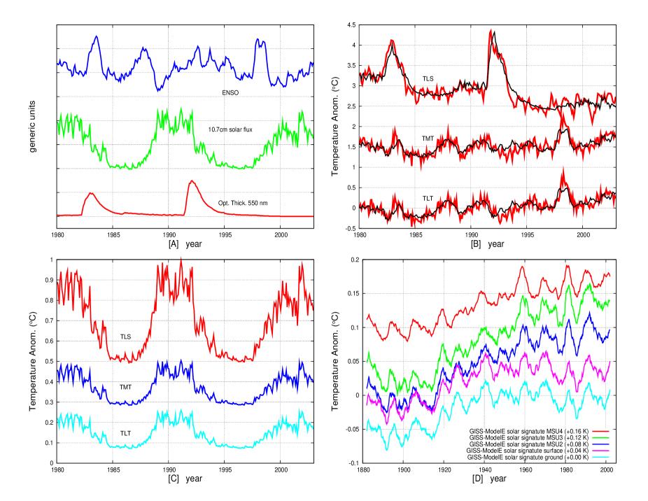
Abbildung 6: (A) Monthly mean optical thickness at 550 nm associated to the volcano signal, the 10.7 cm solar flux values, and the ENSO MEI signals used in the regression model of Eq. (4); (B) Regression model against MSU temperature records: Temperature Lower Troposphere (TLT, MSU 2); Temperature Middle Troposphere (TMT, MSU 2); Temperature Lower Stratosphere (TLS, MSU 4). (C) Solar Signatures as predicted by the regression model Eq. (4). (D) GISS ModelE solar signature prediction from the ground (bottom) to the lower stratosphere (MSU4) (top). Regression coefficients are reported in Table 4.

However, BS09 regression model is also not meaningful for another important physical property. Secular-long climatic sequences cannot be modeled using a linear regression model that directly adopts as linear predictors the radiative forcing functions, as done in BS09, because the climate processes the forcing functions non-linearly by deforming their geometrical shape through its heat capacity. See the discussion in Crowley (2000), Scafetta and West (2005, 2006a, 2006b, 2007) and Scafetta (2009). Essentially, an input radiative forcing function and the correspondent modeled temperature output function do not have the same geometrical shape because each frequency band is processed in different ways (e.g. high frequencies are damped while low frequencies are stretched), and multilinear regression models are extremely sensitive to the shape of the constructors. The same critique applies to Lean and Rind (2009), who also adopted forcing functions as temperature linear predictors to interpret the 20th century warming.

The above problem may be circumvented by using a regression model that uses as predictors theoretical climatic fingerprints of the single forcing functions once processed by an energy balance model, which approximately simulate the climate system, as proposed for example in Hegerl et al. (2003). A simple first approximation choice may be a regression model of the temperature of the type:

$$T(t)=\alpha_{T{{}_{\mathrm{v}}}}T_{\mathrm{V}}(t)+\alpha_{T{{}_{\mathrm{s}}}}T_{\mathrm{S}}(t)+\alpha_{T{{}_{\mathrm{a}}}}T_{\mathrm{A}}(t)+c,$$ (5)

where $T_{\mathrm{v}}(t)$, $T_{\mathrm{S}}(t)$ and $T_{\mathrm{A}}(t)$ are the outputs of an energy balance model forced with the volcano, solar and anthropogenic (GHG plus Aerosol) forcing functions, respectively, and $c$ is a constant. The rationale is the following. Energy balance models provide just a rough modeling of the real climatic feedbacks and processes involved in a specific forcing. What the regression model does is estimate signal amplitudes $\alpha$ (unitless) as scaling factors by which energy balance model simulations need to be scaled for best agreement with observations (Hegerl et al., 2003). This scaling process also makes, in first approximation, the final results approximately independent of the specific energy balance model used to produce the constructors. In particular, the scaling factor is important for determining a first approximation climatic contribution of the overall solar variations which, as explained above, likely present additional forcing (cosmic ray, UV, etc.) functions that present geometrical similarities to the total solar irradiance forcing function alone, but that are not explicitly included in the climate models yet. Indeed, the multiple solar forcings are very likely quasi-multicollinear, which allows the regression model, Eq. (5), to approximately estimate, through the scaling factor $\alpha_{T{{}_{\mathrm{s}}}}$, their overall effect by using only a theoretical climatic fingerprint of one of them.

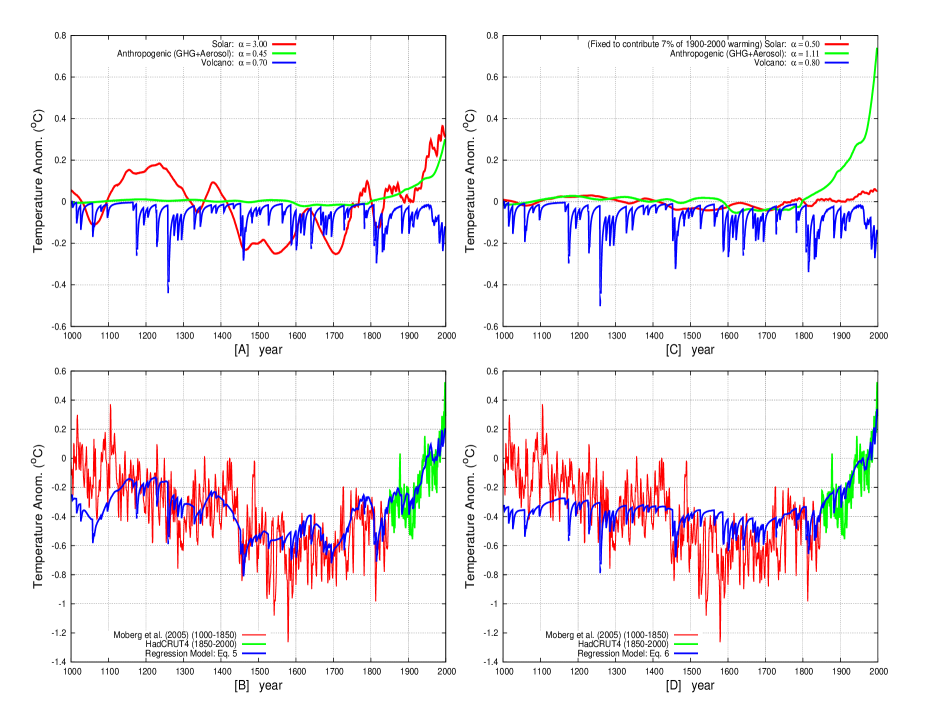
Abbildung 7: (A) Temperature components obtained with the regression model, Eq. (5), using as constructors the energy balance model output functions proposed by Crowley (2000). (B) Comparison between the model Eq. (5) and an estimate of the global surface temperature from 1000 to 2000 AD. The temperature is made of the proxy model by Moberg et al. (2005) (1000–1850, red) and by the HadCRUT4 global surface temperature record (1850–2000, green) Morice et al. (2012). (C) and (D) are like (A) and (B), but here the restricted regression model, Eq. (6), is used, where the solar contribution to the 20th century warming is forced to be 7 % ($0.06$ ^∘C) of the total ($0.8$ ^∘C), as claimed by Benestad and Schmidt (2009). Note that the model, Eq. (6), fails to agree with the temperature before 1750 by not reproducing the great millennial temperature cycle. The regression models appear too rough to properly reconstruct the period 1990-2000.

Because both solar and anthropogenic forcing functions have been increasing since about 1700 (since the Maunder solar minimum and a cold period of the Little Ice Age), to reduce the multicollinearity among the constructors, the regression model should be run against 1000 yr-long temperature records to better take advantage of the geometrical orthogonality between the millennial solar cycle (e.g.: Bond et al., 2001; Kerr, 2001; Ogurtsov et al., 2002; Scafetta, 2012c) and the GHG records. Note that the GHG forcing functions show only a small preindustrial variability and reproduce the shape of a hockey stick (Crowley, 2000). I observe that this crucial point was also not recognized by Rohde et al. (2013, figure 5), who used a regression model of the temperature from 1750 to 2010, and also used predictors equivalent to the forcing functions as in BS09.

In the present example I used the output functions produced by the linear upwelling/diffusion energy balance model from Crowley (2000, figure 3A) in the following way: the volcano output is used as a candidate for the volcano related constructor; the GHG and Aerosol outputs are summed to obtain a comprehensive anthropogenic constructor function; the three solar outputs, which for the 20th century use Lean (2000) solar model, are averaged to obtain an average solar constructor function.

Note that Crowley (2000) and Hegerl et al. (2003) compared their models against hockey-stick temperature reconstructions such as that proposed by Mann et al. (1999), which showed a very little preindustrial variability compared with the post-1900 global warming, and found a relatively small solar signature on climate. However, since 2005, novel paleoclimatic temperature reconstructions have demonstrated a far greater preindustrial variability made of a large millennial cycle with an average cooling from the Medieval Warm Period to the Little Ice Age of about 0.7 ^∘C (Moberg et al., 2005; Mann et al., 2008; Ljungqvist, 2010; Christiansen and Ljungqvist, 2012); the latter cooling is about 3–4 times greater than what showed by the hockey-stick temperature graphs. The example uses the reconstruction of Moberg et al. (2005) assumed to represent a global estimate of the surface temperature, merged in 1850–1900 with the instrumental global surface temperature record HadCRUT4 (Morice et al., 2012).

The result of the analysis are shown in Fig. 7a and b. The evaluated scaling coefficients using Eq. (5) are $\alpha_{T{{}_{\mathrm{v}}}}=0.7$; $\alpha_{T{{}_{\mathrm{s}}}}=3.0$; $\alpha_{T{{}_{\mathrm{a}}}}=0.45$; $c=-0.30$ ^∘C. Figure 7a shows the rescaled energy balance model simulations relative to the three components (volcano, solar and anthropogenic). Figure 7b shows the model, Eq. (5), against the chosen temperature record and a good fit is found. According to the proposed model, from 1900 to 2000 the solar component contributed $\sim 0.35$ ^∘C (44 %) of the total $\sim 0.8$ ^∘C. However, this is likely a low estimate because a fraction (perhaps 10–20 %) of the post-1900 GHG increase may have been a climatic feedback to the solar-induced warming itself through CO₂ and CH₄ released by up-welled water degassing, permafrost melting and other mechanisms. Thus, more likely, the sun may have contributed at least about 50 % of the 20th century warming as found in other empirical studies (e.g.: Eichler et al., 2009; Scafetta and West, 2007; Scafetta, 2009) that more properly interpreted the climate system response to solar changes using long records since 1600 AD, and by taking into account also the scale-by-scale response of the climate system to solar inputs. Indeed, although the regression model appears too rough, Fig. 7a suggests that solar activity and anthropogenic forcings could have contributed almost equally to the global warming observed from 1900 to 2000.

On the contrary, by comparison, Fig. 7c and d show what would have been the situation if the solar contribution to the 20th century warming were only 7 % of the total, that is about $0.06$ ^∘C against $0.8$ ^∘C, as claimed by BS09 and also by the GISS ModelE (see Fig. 6d). Here, I forced the solar component of the regression model to reproduce such a claim, which necessitates a rescaling of Crowley’s solar output $T_{\mathrm{S}}(t)$ by a factor $\alpha_{T{{}_{\mathrm{s}}}}\approx 0.5$. Then, a modification of the regression model of Eq. (5) can be used:

$$T(t)-0.5\cdot T_{\mathrm{S}}(t)=\alpha_{T{{}_{\mathrm{v}}}}T_{\mathrm{V}}(t)+\alpha_{T{{}_{\mathrm{a}}}}T_{\mathrm{A}}(t)+c.$$ (6)

The three regression coefficients are $\alpha_{T{{}_{\mathrm{v}}}}=0.8$, $\alpha_{T{{}_{\mathrm{a}}}}=1.1$ and $c=-0.32$ ^∘C. As Fig. 7c shows, in this case almost the entire 20th century global warming would be interpreted as due to anthropogenic forcings, as all general circulation models of the IPCC (2007) and also Lean and Rind (2009) have claimed. However, as Fig. 7d clearly highlights, the same model, Eq. (6), fails to reproduce the data before 1750 by missing the great millennial oscillation, generating both the Medieval Warm Period (1000–1400) and the Little Ice Age (1400–1750). Equation (6) just reproduces a hockey-stick shape that would only agree well with the outdated paleoclimatic reconstruction by Mann et al. (1999), as also originally found by Crowley (2000).

It is possible to observe that a good agreement between the model, Eq. (6), and the data since 1750 exists, which is the same result found by Rohde et al. (2013, figure 5) with another regression model. These authors concluded that almost all warming since 1750 was induced by anthropogenic forcing. However, Rohde et al. (2013) result is also not robust because their used 260 yr interval (1750–2010) is too short a period, during which both the solar and the anthropogenic forcing functions are collinear (both increased); a regression model therefore cannot properly separate the two signals.

In conclusion, it is evident that the large preindustrial millennial variability shown by recent paleoclimatic temperature reconstructions implies that the sun has a strong effect on the climate system, and its real contribution to the 20th century warming is likely about 50 % of the total observed warming. This estimate is clearly incompatible with BS09’s estimate of a solar contribution limited to a mere 7 % of the 20th century global warming. The result is also indirectly confirmed by the results depicted in Fig. 6, demonstrating that GISS ModelE severely underestimates the solar fingerprints on climatic records by a large factor. For equivalent reasons, by claiming a very small solar effect on climate, the general circulation models used by the IPCC (2007) and the regression models proposed by Rohde et al. (2013) and Lean and Rind (2009), would be physically compatible only with the outdated hockey-stick paleoclimatic temperature graphs (e.g. Crowley, 2000; Mann et al., 1999) if they were extend back to 1000 AD. However, by doing so, they would fail to reproduce the far larger (by a factor of 3 to 4, at least) preindustrial climatic variability revealed by the most recent paleoclimatic temperature reconstruction (e.g.: Christiansen and Ljungqvist, 2012; Kobashi et al., 2013; Ljungqvist, 2010; Mann et al., 2008; Moberg et al., 2005).

3 Maximum overlap discrete wavelet transform, Gibbs artifacts and boundary methods

A technique commonly used to extract structure from complex time series is the maximum overlap discrete wavelet transform (MODWT) multiresolution analysis (MRA) (Percival and Walden, 2000). This methodology decomposes a signal $X(t)$ at the $J$-th order as follows:

$$X(t)=S_{J}(t)+\sum_{j=1}^{J}D_{j}(t),$$ (7)

where $S_{J}(t)$ works as a low-pass filter and captures the smooth modulation of the data with time scales larger than $2^{J+1}$ units of the time interval $\Delta t$ at which the data are sampled. The detail function $D_{j}(t)$ works as a band-pass filter and captures local variation with periods approximately ranging from $2^{j}\Delta t$ to $2^{j+1}\Delta t$. The technique can be used to model the climatic response to different temporal scales of the solar forcing used later to combine the results to obtain a temperature signature induced by solar forcing as proposed in Scafetta and West (2005, 2006a, 2006b).

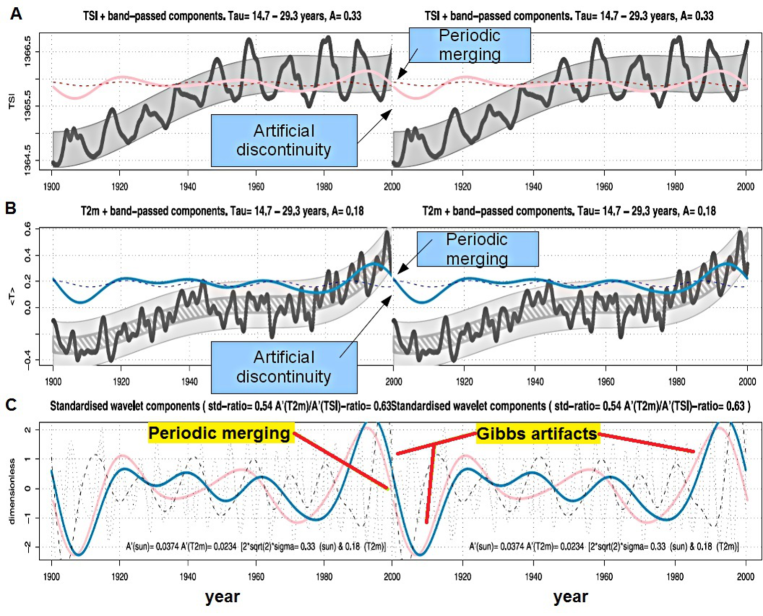
Abbildung 8: Reproduction and comments of Benestad and Schmidt (2009)’s figure 4 applying the MODWT to: (A) a total solar irradiance model (Lean, 2000); (B) the GISTEMP global surface temperature (Hansen et al., 2001). The bottom panel (C) depicts the MODWT decomposed curves (blue and pink) at a time scale of about $\tau=22$ yr. The figure plots the original figure twice, side by side to demonstrate that MODWT was applied improperly with the periodic boundary method.

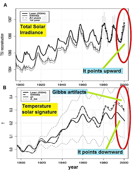
Abbildung 9: Reproduction and comment of Benestad and Schmidt (2009)’s figure 6 (A) and figure 7 (B). The upper panel shows a total solar irradiance model (Lean, 2000); the bottom panel shows its temperature signature produced with the MODWT decomposition at scales larger than the decadal one. The red circles highlight the physical incongruity of the misapplication of the MODWT method by showing that despite the increasing solar activity (upper panel) the wavelet processed curve points downward because of Gibbs artifacts.

However, the MODWT technique needs to be applied with care because the MODWT pyramidal algorithm is periodic (Percival and Walden, 2000). This characteristic implies that to properly decompose a non-stationary time series, such as solar and temperature records, there is the need of doubling the original series by reflecting it in such a way that the two extremes of the new double sequence are periodically continuous: that is, if the original sequence runs from A to B (let us indicate it as “A-B”), it must be doubled to form a sequence of the type “A-BB-A”, which is periodic at the extremes. This boundary method is called “reflection”. If this trick is not applied and the original sequence is processed with the default periodic boundary method, MODWT interprets the sequence as “A-BA-B”, and models the “BA” discontinuities at the extremes by producing Gibbs ringing artifacts that invalidate the analysis and its physical interpretation.

A serious misapplication of the MODWT methodology is also found in Benestad and Schmidt (2009), where they questioned the MODWT results of temperature and solar records found in Scafetta and West (2005, 2006a, 2006b) because they were not able to reproduce them. However, as I will demonstrate below, BS09 misapplied the MODWT by using the periodic boundary method instead of the required reflection one. This error could have been easily recognized by a careful analysis of their results, which were weird. Let us discuss the case.

Figure 8 reproduces BS09’s figure 4, which decomposes with MODWT both a total solar irradiance record (Lean, 2000) and the GISTEMP global surface temperature record (Hansen et al., 2001). Figure 8, however, plots BS09’s figure 4 twice, by merging the 2000 border with the 1900 border side-by-side. As evident in the figure, the original sequences present discontinuities at the borders of the type “A-BA-B” due to their upward trend. However, the MODWT decomposed curves, that is, the pink and blue curves are continuous at the borders. This pattern is generated by the MODWT when the default periodic boundary method is applied. Consequently, very serious Gibbs artifacts are observed in the decomposed curves, as evident in the large oscillations present in the pink and blue curves in proximity of the borders in 1900 and in 2000. These artifacts are also evident in the bottom panel of Fig. 8.

The consequences of the error are quite serious. The Gibbs artifacts induce a large artificial volatility in the decomposed components signals. Moreover, they generated a serious physical incongruity highlighted in Fig. 9a and b. These figures reproduce BS09’s figures 6 and 7, respectively. Here, a total solar irradiance model (Lean, 2000) (Fig. 9a) and its temperature signature reconstruction using the MODWT decomposition methodology of Scafetta and West (2006a) (Fig. 9b) are depicted, respectively. Figure 9a shows that with the MODWT methodology, the solar contribution to the 20th century global warming is about $0.3$ ^∘C (38 %) of the total warming. However, the exact result would be larger if the MODWT were not misapplied and would have fully confirmed Scafetta and West (2006a, b). In fact, the added red circles in Fig. 9 highlight that the solar activity increased from 1995 to 2000 (Fig. 8a), while its temperature reconstructed signature (Fig. 9b) points downward during the same period, which is unphysical. This pattern was due to the fact that the algorithm, as applied by BS09, processed the signal with the default periodic boundary method and generated large Gibbs artifacts trying to merge the starting and the ending points of the record and, consequently, bent the last decade of the reconstructed solar climatic signature downward. Note that in Scafetta and West (2006a, compare figures 2 and 3), where the MODWT was applied correctly using the reflection boundary method, this physical incongruity does not exist. Scafetta and West (2006a, b, 2007) and Scafetta (2009) are consistent also with the results discussed in Sect. 3 and Figure 7 where it was determined that the sun contributed about 50% of the global warming from 1900 to 2000 using an independent methodology.

Let us discuss how to correctly apply the MODWT methodology as used in Scafetta and West (2005, 2006a) to capture the 11 yr and 22 yr solar cycle signatures. In addition to the reflection method for mathematical purposes, MODWT methodology has to be used under the following two conditions for physical reasons: (1) the data record needs to be resampled in such a way that the center of the wavelet band-pass filter is located exactly on the 11 and 22 yr solar cycles, which are the frequencies of interest; (2) a reasonable choice of the year when the reflection is made, that is, the year 2002–2003 when the sun experienced a maximum for both the 11 yr and 22 yr cycles to further reduce a problem of discontinuity in the derivative at the border because there is the need to apply MODWT with the reflection method.

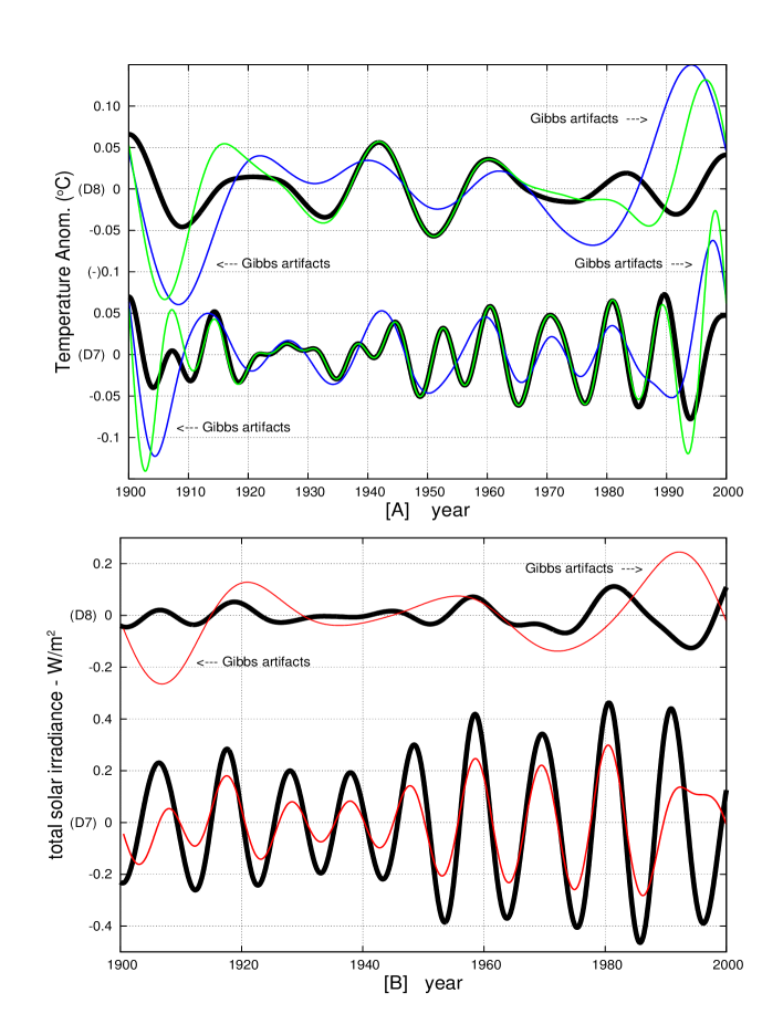
Abbildung 10: (A) MODWT of the GISTEMP dataset (Hansen et al., 2001) from 1900 to 1999. (Top) Detail curve $D_{8}$; (Bottom) Detail curve $D_{7}$. The thick black curves are the correct $D_{7}$ and $D_{8}$ wavelet detail curves obtained with reflection boundary condition and the correct time step of $\Delta t=0.6875$ month. The thin blue lines “exactly” correspond to the curves depicted in Fig. 8 in blue (central panel) and blue and dash (bottom panel). The thin green lines are obtained using the periodic method and the correct time step of $\Delta t=0.6875$ month. (B) MODWT of the (Lean, 2000) TSI from 1900 to 1999. (Top) Detail curve $D_{8}$; (Bottom) Detail curve $D_{7}$. The thick black curves are the correct $D_{7}$ and $D_{8}$ wavelet detail curves obtained with reflection boundary condition and the correct time step of $\Delta t=0.6875$ month. The thin red curve in the upper panel “exactly” corresponds to the curves reported in Fig. 8 in pink (upper and bottom panels) that were obtained by using the cyclical periodic boundary condition and the incorrect time step of $\Delta t=1$ month.

Point (1) was accomplished by observing that the 11 yr cycle (132 months) would fall within the frequency band captured by the wavelet detail $D_{7}(t)$ corresponding to the band between $2^{7}=128$ and $2^{8}=256$ months, that is from 10.7 to 21.3 yr. Thus, by adopting the monthly sampling the 11 yr cycle would not be centered in $D_{7}(t)$ and the 22 yr would not be centered in the wavelet detail $D_{8}(t)$. This would cause an excessive splitting of the 11 yr modulation between the adjacent details curve $D_{6}(t)$ and $D_{7}(t)$, and of the 22 yr modulation between the adjacent detail curves $D_{7}(t)$ and $D_{8}(t)$. Consequently, to optimize the filter it was necessary to adjust the time step of the time sequence in such a way that the wavelet detail curves fell exactly in the middle of the 11 yr and 22 yr cycles. This was done by adjusting the time sampling of the record to $\Delta t=132/192=0.6875$ month or to $\Delta t=11/12=0.9167$ yr whether the original sequence has a monthly or annual resolution, respectively. This time step adjustment was accomplished with a simple linear interpolation of the original sequence. With the new resolution $\Delta t=0.6875$ month, the detail curve $D_{7}(t)$ would cover the timescales 7.3–14.7 yr (median 11 yr), and the detail curve $D_{8}(t)$ would cover the timescales 14.7–29.3 yr (median 22 yr). This time step is necessary to optimally extract the 11 yr and 22 yr modulations from the data.

Tabelle 5: Comparison of the amplitudes of the detail curves shown in Fig. 10 calculated by fitting with function $f(x,P)=0.5A\cos(2\pi(x-T)/P)$, whe the period $P$ is chosen to be 11 yr for $D_{7}$ or for 22 yr for $D_{8}$. First column shows the amplitudes $A$ for the period 1980–2000 using the correct reflection method and the optimized time sampling $\Delta t=0.6875$ month. Second column shows the amplitudes $A$ for the period 1980–2000 using the incorrect periodic method and the non-optimized time sampling $\Delta t=1$ month. Third column shows the values as calculated in Benestad and Schmidt (2009), which are more similar to those listed in column 2.

	Reflection (correct)	Periodic (incorrect)	BS09
$A_{\mathrm{8,temp}}$	$0.057\pm 0.0015$ ∘C	$0.193\pm 0.002$ ∘C	$0.18$ ∘C
$A_{\mathrm{8,sun}}$	$0.226\pm 0.003$ W m-2	$0.266\pm 0.0025$ W m-2	$0.32$ W m-2
$A_{\mathrm{8,temp}}/A_{\mathrm{8,sun}}$	$0.252\pm 0.010$ ∘C W-1 m2	$0.726\pm 0.014$ ∘C W-1 m2	$0.56$ ∘C W-1 m2
$A_{\mathrm{7,temp}}$	$0.112\pm 0.005$ ∘C	$0.077\pm 0.010$ ∘C	$0.14$ ∘C
$A_{\mathrm{7,sun}}$	$0.872\pm 0.008$ W m-2	$0.292\pm 0.021$ W m-2	$0.45$ W m-2
$A_{\mathrm{7,temp}}/A_{\mathrm{7,sun}}$	$0.128\pm 0.007$ ∘C W-1 m2	$0.264\pm 0.053$ ∘C W-1 m2	$0.311$ ∘C W-1 m2

Figure 10a shows the MODWT decomposition of the GISTEMP temperature record from 1900 to 2000. The thick black curves are the $D_{7}$ (bottom) and $D_{8}$ (top) wavelet detail curves obtained with the reflection method and the correct time step $\Delta t=0.6875$ month. A second set of curves are also depicted in Fig. 10a and these are obtained from the same data, but using cyclic boundary conditions and with $\Delta t=1$ month (blue) and $\Delta t=0.6875$ month (green). The blue and green curves of Fig. 10a show substantial Gibbs ringing artifacts that are so serious that they even cause an inversion of the bending of the curve. The blue curves exactly correspond to the blue (middle panel) and to the blue and dash (bottom panel) curves depicted in Fig. 8, as calculated by BS09 where these Gibbs artifacts were mistakenly identified as anomalous temperature and solar signatures. The re-analysis also demonstrates that the calculations by BS09 used the $\Delta t=1$ month resolution, contrary to what they report in their figure 4.

The consequences of the error of using MODWT with the default periodic method are significant. For example, the MODWT detail curves were used to estimate the average peak-to-trough amplitudes $A$ of the oscillations from 1980 to 2000. The blue curves for $D_{8}$ gives $A_{\mathrm{8,temp}}\approx 0.19$ ^∘C, while the value determined using the correct analysis is $A_{\mathrm{8,temp}}\approx 0.06$ ^∘C corresponding to the one obtained in Scafetta and West (2005). Note also that from 1980 to 2000 the blue curve referring to $D_{8}$ is concave while the correct curve (black) is convex. Analogous problem referring to $D_{8}$ is shown in Fig. 10b that analyzes the total solar irradiance of Lean (2000). Again the thick black curves are the $D_{7}$ (bottom) and $D_{8}$ (top) wavelet detail curves obtained with the reflection method and the centered time step $\Delta t=0.6875$ month. The thin red lines correspond to the pink curves of Fig. 8. These latter curves are quite different from the black curves because of Gibbs artifacts and because the $\Delta t=1$ month resolution was used. In particular, notice the visibly smaller amplitude of the 11 yr solar cycles relative to the correct black curve: with BS09’s methodology one would find $A_{\mathrm{7,sun}}=0.3$ W m^-2 while the correct amplitude is significantly larger $A_{\mathrm{7,sun}}\approx 0.9$ W m^-2 since 1980, as found in Scafetta and West (2005). Moreover, as Fig. 4a clearly shows, from 1900 to 2000 the amplitude of the 11-year solar cycle varies from $0.5$ to $1.3$ about W m^-2 and this range is clearly inconsistent with the average amplitude of $0.45$ W m^-2 as calculated in BS09. The various amplitudes are listed in Table 5, which also highlights the abnormal results obtained in BS09.

In summary, MODWT requires: (1) the reflection method; (2) the sequences should be sampled at specific optimized time intervals that depend on the specific application; (3) for optimal results the borders need to be chosen to avoid discontinuities in the first derivative at the time scales of interest. For example, Scafetta and West (2005) used the period 1980–2002 because the 11 yr and 22 yr solar cycles would approximately have been at their maximum. The latter point is important because the reflection method gives optimized results when the derivative at the borders approaches zero. On the contrary, choosing the default periodic method and using sequences sampled at generic time intervals and generic borders, as done in BS09, was demonstrated here to yield results contaminated by significant artifacts.

There are other claims raised in BS09 as those based on GISSModelE and GISS CTL simulations simulations, etc. However, in Sect. 3 it has been also demonstrated that these simulations do not reproduce the solar and astronomical signatures on the climate at multiple time scales (see also Scafetta, 2010, 2012b) and would eventually agree only with the outdated hockey-stick temperature reconstructions such as those proposed by Mann et al. (1999). Therefore, BS09’s additional arguments are of limited utility (1) because those computer simulations appear to seriously underestimate the solar signature on climate and (2) because, in any case, BS09 misapplied the MODWT methodology to analyze them.

In this paper I have discussed a few typical examples where time series methodologies used to analyze climatic records have been misapplied. The chosen examples address relatively simple situations that yielded severe physical misinterpretations that, perhaps, could have been easily avoided.

A first example addressed the problem of how to estimate accelerations in tide gauge records. It has been shown that to properly interpret the tide gauge record of New York City it is necessary to plot all available data since 1856, as done in Fig. 3b. In this way the existence of a quasi 60 yr oscillation, which is evident in the global sea level record since 1700, becomes quite manifest. This pattern suggests a very different interpretation than that proposed for example in Sallenger Jr. et al. (2012) or in Boon (2012). A significantly smaller and less alarming secular acceleration in NYC was found: $a=0.006\pm 0.005$ mm yr^-2 against Sallenger Jr. et al. (2012)’s 1950–2009 and 1970–2009 accelerations $a=0.044\pm 0.03$ mm yr^-2 and $a=0.13\pm 0.09$ mm yr^-2, respectively, or Boon’s (2012) 1969–2011 acceleration $a=0.20\pm 0.07$ mm yr^-2. These large accelerations simply refer to the bending of the quasi 60 yr natural oscillation present in this record: see Scafetta (2013) for additional details. Thus, in NYC a more realistic sea level rise projection from 2000 to 2100 would be about $350\pm 30$ mm instead of $1130\pm 480$ mm calculated with Sallenger Jr. et al. (2012)’s method using the 1970–2009 quadratic polynomial fit or $1550\pm 400$ mm calculated with Boon’s (2012) method using the 1969–2011 quadratic polynomial fit. Moreover, as Fig. 1a shows, by plotting the NYC tide gauge record only since 1950 (compare Figs. 1a and 3b), Sallenger Jr. et al. (2012) has somehow obscured the real dynamics of this record; the same critique would be even more valid for Boon (2012, figures 5–8) who plotted tide gauge records only starting in 1969.

Global sea level may rise significantly more if during the 21st century the temperature increases abnormally by several degrees Celsius, as current general circulation models have projected (Morice et al., 2012). However, as demonstrated in Sect. 3 (e.g. Figs. 6 and 7) typical climate models used for these projections appear to significantly overestimate the anthropogenic warming effect on climate and underestimate the solar effect. Solar activity is projected to decrease during the following decades and may add a cooling component to the climate (Scafetta, 2012c; Scafetta and Willson, 2013). As a consequence, it is very likely that the 21st century global temperature projections are too high, as also demonstrated in Scafetta (2012b). Because the global sea level record presents a 1700–1900 preindustrial period acceleration compatible with the 1900–2000 industrial period acceleration ($a=\sim 0.01$ mm yr^-2 in both cases), there is no clear evidence that anthropogenic forcings have drastically increased the sea level acceleration during the 20th century. Thus, anthropogenic forcings may not drastically increase the sea level during the 21th century either. The 1700–2000 global sea level is projected to rise about $277\pm 8$ mm from 2000 to 2100 as shown in Fig. 2a.

A second example addressed more extensively the problem of how to deal with multilinear regression models. Multilinear regression models are very powerful, but they need to be used with care to avoid multicollinearity among the constructors yielding meaningless physical interpretations. It has been demonstrated that the 10-constructor multi-linear regression model adopted in Benestad and Schmidt (2009) to interpret the 20th century global warming and to conclude that the sun contributed only 7 % of the 20th century warming is not robust because: (1) the used predictors are multicollinear and (2) the climate is not a linear superposition of the forcing functions themselves. About the latter point, it is evident that if the climate system could be interpreted as a mere linear superposition of forcing functions (as also done in Lean and Rind (2009)), there would be no need to use climate models in the first place.

To demonstrate the serious artifacts generated by regression analyses in multicollinearity cases, I showed that by eliminating the predictor claimed to be the most responsible for the observed global warming from 1900 to 2000, that is the well-mixed greenhouse gas forcing function, the regression model was still able to reconstruct equally well the temperature record by using the other 9 constructors. By using the regression model in a more appropriate way, that is, by restricting the analysis to the 1980–2003 period when the data are more accurate and using only orthogonal constructors, it was demonstrated that the GISS ModelE severely underestimates the solar effect on climate by a 3-to-8 factor, as shown in Fig. 6. By using a more physically based regression model (Eq. 5) it was also demonstrated that the large preindustrial temperature variability shown in recent paleoclimatic temperature reconstructions since the Medieval Warm Period implies that the sun has a strong effect on climate change and likely contributed about 50 % of the 20th century warming, as found in numerous Scafetta’s papers (Scafetta and West, 2006a, b, 2007; Scafetta, 2009, 2010, 2012a, 2012b) and by numerous other authors (e.g.: Eichler et al., 2009; Hoyt and Schatten, 1993; Kirkby, 2007; Kobashi et al., 2013; Soon, 2005; Soon et al., 2011; Soon and Legate, 2013; Svensmark, 2007). These results contradict Benestad and Schmidt (2009), IPCC (2007), Lean and Rind (2009) and Rohde et al.’s (2013) results that the sun contributed little (less than 10 %) to the $0.8$ ^∘C global warming observed from 1900 to 2000. In fact, such a low solar contribution would only be consistent with the geometrical patterns present in outdated hockey-stick temperature reconstructions (e.g. those proposed in: Crowley, 2000; Mann et al., 1999), as shown in Fig. 7.

A third example addressed the problem of how to deal with scale-by-scale wavelet decomposition methodologies, which are very useful to interpret dynamical details in geophysical records. Evidently, there is a need to properly take into account the mathematical properties of the methodology to avoid embarrassing artifacts and physical incongruities as those generated by Gibbs artifacts. For example, Benestad and Schmidt (2009) findings that the solar activity increase from 1995 to 2000 has induced a cooling on the global climate and their failure to reproduce the results of Scafetta and West (2005, 2006a, 2006b) were just artifacts due to an improper application of the MODWT technique. Benestad and Schmidt (2009) erroneously applied MODWT with the default period method instead of using the reflection method as demonstrated in Figs. 8–10. The error in applying correctly the decomposition methodology also produced abnormally large uncertainties in their results. I have spent some time to detail how to use this technique for the benefit of the readers interested in properly applying it.

Highlighting these kinds of problems is important in science. In fact, while errors in scientific research are sometimes possible and unavoidable, what most harms the scientific progress is the persistence and propagation of the errors. This happens when other scientists uncritically cite and use the flawed results to interpret alternative data, which yields further misinterpretations. This evidently delays scientific progress and may damage society as well.