On the characterization of some classes
of proximally smooth sets

Abstract.

We provide a complete characterization of closed sets with empty interior and positive reach in $\mathbb{R}^{2}$. As a consequence, we characterize open bounded domains in $\mathbb{R}^{2}$ whose high ridge and cut locus agree, and hence $C^{1}$ planar domains whose normal distance to the cut locus is constant along the boundary. The latter results extends to convex domains in $\mathbb{R}^{n}$.

1. Introduction

A nonempty closed subset $S$ of $\mathbb{R}^{n}$ is called proximally smooth, or with positive reach, if for every point $x$ belonging to an open tubular neighborhood outside $S$ there is a unique minimizer of the distance function from $x$ to $S$.

These sets were introduced in 1959 in the seminal paper [29] by Federer, who also proved many of their most relevant properties, in particular the validity of a tube formula, which expresses the Lebesgue measure of a sufficiently small $r$-parallel neighborhood of a set with positive reach in $\mathbb{R}^{n}$ as a polynomial in $r$ of degree $n$.

The concept of proximal smoothness can in fact be located at the crossroad of different areas, such as Geometric Measure Theory, Convex Geometry, Nonsmooth Analysis, Differential Geometry. Since Federer, it has been investigated and developed in various ways. Related research directions include generalized Steiner-type formulae, tubular neighborhoods, and curvature measures [17, 34, 35, 41, 45]; connections with Lipschitz functions, semi-concave functions, and lower-$C^{2}$ functions [16, 32]; proximal smoothness in abstract frameworks, such as Banach spaces or Riemannian manifolds [5, 7]; applications to nonlinear control systems and differential inclusions [11, 18, 19].

More comprehensive accounts of results in this area and related bibliography can be found in the surveys papers [20, 43].

In this paper we are concerned with the following question:

(*) Which is the geometry of a closed set $S\subset\mathbb{R}^{2}$ with positive reach and empty interior?

As far as we are aware, no previous contributions are available in this respect in the literature. In particular, it is worth advertising that one cannot apply the several existing results which allow to retrieve regularity information on a set starting from the regularity of its distance function (possibly squared or signed). Indeed, some of these results are classical and some others are more recent (see e.g. [4, 6, 28, 33]), but in any case they rely on some regularity assumption on the distance up to the involved set. In spite, by definition, the distance function from a set $S$ of positive reach is required to be differentiable just on the set of points where it is sufficiently small and strictly positive, thus not necessarily on $S$ itself (see Definition 1).

Our main results provide a complete answer to question (*): each connected component of $S$ is either a singleton or a manifold of class $C^{1,1}$ (see Theorem 2); in case the distance from $S$ is at least $C^{2}$ in an open neighborhood of $S$, then such manifolds have no boundary and are of class $C^{2}$ (see Theorem 3); moreover, in case the distance from $S$ goes beyond the $C^{2}$ threshold, $S$ gains the same regularity (see Remark 4).

As a by-product, we are able to answer the following related question:

(**) Which is the geometry of a set $\Omega\subset\mathbb{R}^{2}$ whose high ridge and cut locus agree?

Recall that, given an open bounded domain $\Omega\subset\mathbb{R}^{2}$, the high ridge is the set of points where the distance function from $\partial\Omega$ attains its maximum over $\overline{\Omega}$, while the cut locus is the closure in $\overline{\Omega}$ of the so-called skeleton, namely of the sets of points in $\Omega$ which admit multiple closest points on $\partial\Omega$; recall also that the central set is formed by the centers of the maximal disks contained into $\Omega$. We refer to Section 2 for the precise formulation of these definitions. All these sets, which have each one its own role in the geometry of the distance function from the boundary, have been widely investigated in the literature, often with a non-uniform terminology. A miscellaneous collection of related references, without any attempt of completeness, is [1, 3, 9, 26, 30, 31, 38, 39]. It must be added that recently the singular set of the distance function has raised an increasing interest also in applied domains, such as computer science and visual reconstruction, and this is especially true for the central set (often named medial axis in this context), see e.g. [8, 14, 27, 44] and Remark 8 below.

To pinpoint the link between questions (*) and (**), one has to observe that, if the cut locus and high ridge of a domain $\Omega$ coincide, they can be identified with a proximally smooth set with empty interior. As a consequence, the answer to question (**) is: $\Omega$ is the outer parallel neighborhood of a $C^{1,1}$ manifold; in particular, if $\Omega$ is assumed to be of class $C^{2}$ and simply connected, it must be necessarily a disk (see Theorem 6).

We remark that our answer to question (**) solves also the problem of characterizing domains of class $C^{1}$ whose normal distance to the cut locus is constant along the boundary (see Corollary 10). Intuitively, the normal distance of a point $y\in\partial\Omega$ measures how far one can enter into $\Omega$ starting at $y$ and moving along the direction of the inner normal before hitting the cut locus; the precise definition is recalled in Section 2. This notion has been considered from different points of views: in [10, 36, 37] the regularity of the normal distance under different requirements on the boundary has been investigated, along with some applications to Hamilton-Jacobi equations and to PDEs related with granular matter theory; in [13, 23, 24, 25] the normal distance has been exploited in order to study the minimizing properties of the so-called web functions. Let us also mention that, in a previous paper, we proved a roundedness criterion based on the constancy along the boundary of a $C^{2}$ domain of a certain function, depending on the normal distance and on the principal curvatures, see [21, Thm. 1]. If compared to such result, the roundedness criterion stated in Corollary 10 of the present paper has the advantages of applying to any $C^{1}$ domain, and of involving uniquely the normal distance; moreover, it is obtained through completely different techniques, of more geometrical nature.

We conclude by observing that clearly questions (*) and (**) can be raised also in space dimensions higher than $2$ (or even in a Riemannian manifold), but they seem much more difficult to solve. Nonetheless, concerning question (**), we are able to deal with domains in the $n$-dimensional Euclidean space, under the severe restriction that they are convex (see Theorem 12). Removing this restriction remains by now an open problem.

We defer to a companion paper [22] some applications of the geometric results contained in this manuscript to PDEs, specifically to boundary value problems involving the infinity-Laplacian operator.

The outline of the paper is the following: hereafter we fix some notation; in Section 2 we state the main results; in Section 3 we provide some background material; Section 4 is devoted to some intermediate key results, which prepare the proofs given in Section 5.

Acknowledgments. The authors would like to thank Piermarco Cannarsa for pointing out the paper [1].

Notation. The standard scalar product of two vectors $x,y\in\mathbb{R}^{n}$ is denoted by $\left\langle x,\,y\right\rangle$, and $|x|$ stands for the Euclidean norm of $x\in\mathbb{R}^{n}$. Given an open bounded domain $\Omega\subset\mathbb{R}^{n}$, we denote by $|\Omega|$ and $|\partial\Omega|$ respectively its $n$-dimensional Lebesgue measure and the $(n-1)$-dimensional Hausdorff measure of its boundary. We set $\Omega^{c}:=\mathbb{R}^{n}\setminus\Omega$.

We call $B_{r}(p)$ the open disk of center $p$ and radius $r$, and $\overline{B}_{r}(p)$ its closure. We indicate by $[p,q]$ the line segment with extremes $p$ and $q$.

As customary, we say that a function is of class $C^{k,\alpha}$ when all its derivatives up to order $k$ satisfy a Hölder condition of exponent $\alpha$, and that it is of class $C^{\omega}$ when it is analytic.

By saying that an open set $\Omega\subset\mathbb{R}^{n}$ (or, equivalently, its closure $\overline{\Omega}$ or its boundary $\partial\Omega$) is of class $C^{k}$, $k\in\mathbb{N}$, we mean that, for every point $x_{0}\in\partial\Omega$ there exists a neighborhood $U$ of $x_{0}$ and a bijective map $\psi\colon B_{1}(0)\to U$ such that $\psi\in C^{k}(B_{1}(0))$, $\psi^{-1}\in C^{k}(U)$, $\psi(B_{1}(0)\cap\{x_{n}>0\})=\Omega\cap U$, $\psi(B_{1}(0)\cap\{x_{n}=0\})=\partial\Omega\cap U$. An analogous definition holds with $C^{k,\alpha}$, $C^{\infty}$, $C^{\omega}$ instead of $C^{k}$.

Given a closed set $S\subset\mathbb{R}^{n}$, we denote by $d_{S}$ the distance function from $S$, defined by

$$d_{S}(x):=\min_{y\in S}|x-y|,\quad x\in\overline{\Omega}\ ,$$

where $|\cdot|$ is the Euclidean norm in $\mathbb{R}^{n}$, and by $\pi_{S}$ the projection map onto $S$, namely, for every $x\in\mathbb{R}^{n}$, we call $\pi_{S}(x)$ the set of points $y\in S$ such that

$$|x-y|=d_{S}(x)\,.$$

Whenever $x$ has a unique projection onto $S$, with a minor abuse of notation we shall identify the set $\pi_{S}(x)$ with its unique element.

Moreover, for $r>0$ we denote by $S_{r}$ the $r$-tubular neighborhood of $S$:

$$S_{r}:=\big{\{}x\in\mathbb{R}^{n}\ :\ d_{S}(x)<r\big{\}}\ .$$

2. Main results

Definition 1.

We say that a set $S\subset\mathbb{R}^{n}$ is proximally $C^{k}$ (of radius $r_{S}$) if it is nonempty, closed, and there exists $r_{S}>0$ such that the distance function $d_{S}$ is of class $C^{k}$ in the set $\{x\in\mathbb{R}^{n}\ :\ 0<d_{S}(x)<r_{S}\}$.

Notice that proximally $C^{1}$ sets according to the above definition correspond to sets which in the literature are usually named proximally smooth, or with positive reach, as discussed in the Introduction.

Our main results are the following characterizations of planar sets $S$ which satisfy one of the following conditions:

• $S\subset\mathbb{R}^{2}$ is connected, with empty interior, proximally $C^{1}$;

• $S\subset\mathbb{R}^{2}$ is connected, with empty interior, proximally $C^{2}$.

Theorem 2.

Assume that $S\subset\mathbb{R}^{2}$ satisfies $(H1)$.

Then $S$ is either a singleton, or a $1$-dimensional manifold of class $C^{1,1}$.

Theorem 3.

Assume that $S\subset\mathbb{R}^{2}$ satisfies $(H2)$.

Then $S$ is either a singleton, or a $1$-dimensional manifold without boundary of class $C^{2}$.

Remark 4.

(i) Clearly, if the assumption $S$ connected is removed from $(H1)$ and $(H2)$, Theorems 2 and 3 can be applied to characterize each connected component of $S$.

(ii) If the assumption $S$ bounded is added to $(H2)$, Theorem 3 allows to conclude that $S$ is a regular simple closed curve of class $C^{2}$.

(iii) If the regularity requirement in condition $(H2)$ is strengthened by asking that $S$ satisfies Definition 1 with $C^{2}$ replaced either by $C^{k,\alpha}$, for some $k\geq 2$ and $\alpha\in[0,1]$, or by $C^{\infty}$, or by $C^{\omega}$, then the thesis of Theorem 3 can be strengthened accordingly, namely the manifold $S$ turns out to be respectively of class $C^{k,\alpha}$, $C^{\infty}$, or $C^{\omega}$ (cf. Remark 23).

(iv) It is a natural question to ask whether Theorem 2 still holds if the condition $S$ proximally $C^{1}$ is weakened into an exterior sphere condition. Namely, if $S$ is proximally $C^{1}$ of radius $r_{S}$, for every $r\in(0,r_{S})$, every $x\in S$ and every unit vector $\zeta$ such that $x\in\pi_{S}(x+r\zeta)$, the ball of radius $r$ centered at $x+r\zeta$ does not intersect $S$ (see e.g. [16, Thm. 4.1 (d)]). At least without any additional assumption on $S$, the converse implication is not true: the exterior sphere condition is strictly weaker than proximal smoothness (see [40]), and it turns out that it is not sufficient to guarantee the validity of Theorem 2. Examples of sets which satisfy an exterior sphere condition but are not a manifold of class $C^{1,1}$, or not a manifold at all, can be easily constructed: think for instance to the graph of the function $|x|$, or to the union of two mutually tangent circumferences.

We now turn attention to the consequences of Theorems 2 and 3 on the geometry of planar domains whose high ridge and cut locus coincide. We are going to see that such domains admit a simple geometrical characterization, as tubular neighborhoods of a $C^{1,1}$ manifold; moreover such characterization turns into a symmetry statement in case the involved domain is $C^{2}$ and simply connected.

In order to state these results more precisely, and since the terminology adopted in this respect in the literature is not uniform, let us fix some notation concerning the geometry of the distance function from the boundary.

Definition 5.

Let $\Omega\subset\mathbb{R}^{n}$ be an open bounded domain.

– $\Sigma(\Omega)$:= the skeleton of $\Omega$ is the singular set of $d_{\partial\Omega}$ (i.e., the set of points $x\in\Omega$ such that $d_{\partial\Omega}$ is not differentiable at $x$, or equivalently such that $\pi_{\partial\Omega}(x)$ is not a singleton);

– $\operatorname{\overline{\Sigma}}(\Omega)$:= the cut locus of $\Omega$ is the closure of $\Sigma(\Omega)$ in $\overline{\Omega}$;

– $\operatorname{C}(\Omega)$:= the central set of $\Omega$ is the set of the centers of all maximal balls contained into $\Omega$. (We say that an open ball $B_{r}(p)$ is a maximal ball contained into $\Omega$ if $B_{r}(p)\subset\Omega$ and there does not exist any other open ball strictly containing $B_{r}(p)$ which is still contained into $\Omega$.)

– $\operatorname{M}(\Omega)$:= the high ridge of $\Omega$ is the set where $d_{\partial\Omega}$ attains its maximum over $\overline{\Omega}$ .

Several topological and structure properties of these sets are known; some of them, which will be needed somewhere in the paper, are recalled in Section 3 (see Proposition 14). Here let us just recall that, for a general domain $\Omega$, there holds

(1) $$\operatorname{M}(\Omega)\subseteq\Sigma(\Omega)\subseteq\operatorname{C}(\Omega)\subseteq\operatorname{\overline{\Sigma}}(\Omega).$$

Indeed, the inclusion $\operatorname{M}(\Omega)\subseteq\Sigma(\Omega)$ follows immediately from the eikonal equation; for the remaining inclusions see [30, Thm. 3B].

We point out that these inclusions may be strict. Simple examples are the following: when $\Omega=R$ is a rectangle one has

$$\operatorname{M}(R)\subsetneq\Sigma(R)=\operatorname{C}(R)\subsetneq\operatorname{\overline{\Sigma}}(R),$$

while $\Omega=E$ is an ellipse one has

$$\operatorname{M}(E)\subsetneq\Sigma(E)\subsetneq\operatorname{C}(E)=\operatorname{\overline{\Sigma}}(E).$$

More pathological examples, where these sets turn out to be “substantially” different, are indicated in Remark 15 below.

We now turn our attention to the question stated as (**) in the Introduction: what can be said about planar domains $\Omega$ for which all the inclusions in (1) become equalities? The answer is contained in the next statement.

Theorem 6.

Let $\Omega\subset\mathbb{R}^{2}$ be a nonempty open bounded connected domain such that

(2) $$\operatorname{M}(\Omega)=\operatorname{\overline{\Sigma}}(\Omega)=:S\,.$$

Then $S$ is either a singleton or a $1$-dimensional manifold of class $C^{1,1}$ and, setting $\rho_{\Omega}:=\max_{\overline{\Omega}}d_{\partial\Omega}$, $\Omega$ is the $\rho_{\Omega}$-tubular neighborhood

$$\Omega=S_{\rho_{\Omega}}:=\{x\in\mathbb{R}^{2}\ :\ d_{S}(x)<\rho_{\Omega}\}\,.$$

In particular, if $\Omega$ is $C^{2}$, then $S$ is either a singleton or a $1$-dimensional manifold without boundary of class $C^{2}$, and $\Omega=S_{\rho_{\Omega}}$.

Finally, if $\Omega$ is also simply connected, then $S$ is a singleton, and $\Omega$ is the disk with center $S$ and radius $\rho_{\Omega}$.

Remark 7.

By inspection of the proof of Theorem 6, it follows that, for every $r\in(0,\rho_{\Omega})$, the parallel set

$$S_{r}:=\big{\{}x\in\mathbb{R}^{2}\ :\ d_{S}(x)<r\big{\}}$$

is of class $C^{1,1}$. We point out that this is not necessarily true also for $r=\rho_{\Omega}$. In other words, a domain $\Omega$ satisfying the assumptions of Theorem 6 does not need to be of class $C^{1,1}$, nor $C^{1}$. For instance, let $p:=(-1,1)$, $q:=(0,1)$, $a:=(1,0)$, $b:=(1,-1)$, and define $S$ by

$$S:=[p,q]\cup\big{\{}\partial B_{1}(0)\cap\{x_{1}\geq 0,x_{2}\geq 0\}\big{\}}\cup[a,b]\,.$$

Then the $1$-tubular neighbourhood of $S$, namely $\Omega=\big{\{}x\in\mathbb{R}^{2}\,:\,d_{S}(x)<1\big{\}}$ satisfies the assumptions of Theorem 6, and in particular condition (2), but is not of class $C^{1}$ (see Figure 1 left).

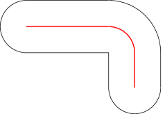
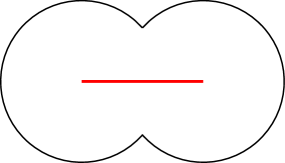
Figure 1. The sets described in Remarks 7 and 11.

Remark 8.

Using the notation of [27], a maximal disk $D$ in $\Omega$ is said to be regular if the contact set $\partial D\cap\partial\Omega$ contains exactly two points, and singular if this is not the case. Then, if $\Omega$ satisfies the assumptions of Theorem 6, and denoting by $S^{*}$ the (possibly empty) boundary of the manifold $S$, we have that all maximal disks centered at $S\setminus S^{*}$ are regular, while the ($0$ or $2$) maximal disks centered at $S^{*}$ are singular.

Let us now restrict attention to domains $\Omega$ of class $C^{1}$. For such a domain, let $\nu_{\Omega}$ denote the inner unit normal to $\partial\Omega$, and let us recall the following definition of normal distance:

Definition 9.

Let $\Omega\subset\mathbb{R}^{n}$ be an open bounded domain of class $C^{1}$. For every $y\in\partial\Omega$, its normal distance to the cut locus is given by

$$\lambda_{\Omega}(y):=\sup\big{\{}t\geq 0\ :\ \pi_{\partial\Omega}(y+t\nu_{\Omega}(y))=\{y\}\big{\}}\ ,$$

As a consequence of Theorem 6, we are able to characterize planar domains $\Omega$ of class $C^{1}$ with constant normal distance along the boundary:

Corollary 10.

Let $\Omega\subset\mathbb{R}^{2}$ be an open bounded connected domain of class $C^{1}$ such that, for all $y\in\partial\Omega$,

(3) $$\lambda_{\Omega}(y)=\text{constant}\,.$$

Then $\Omega$ satisfies $(\ref{f:ug})$ and hence its geometry can be characterized according to Theorem 6.

Remark 11.

We point out that the assumption $\Omega\in C^{1}$ in Corollary 10 cannot be weakened. To be more precise notice first that, if $\Omega$ is just piecewise $C^{1}$, Definition 9 of the function $\lambda_{\Omega}$ can still be given for $y$ belonging to $\partial\Omega$ except a finite number of points (those where $\nu_{\Omega}$ is not defined). Nevertheless, if equality (3) is valid only ${\mathcal{H}}^{1}$-a.e. on $\partial\Omega$, the geometric condition $\operatorname{M}(\Omega)=\operatorname{\overline{\Sigma}}(\Omega)$ is not necessarily true. For instance, let $\alpha>0$, let $r\in(\alpha,2\alpha)$, and let $\Omega:=B_{r}(p)\cup B_{r}(q)$, where $p:=(-\alpha,0)$, and $q:=(\alpha,0)$ (see Figure 1 right). Then we have $\lambda_{\Omega}(y)=r$ for all $y\in\partial\Omega\setminus\big{(}\partial B_{r}(p)\cap\partial B_{r}(q))$, but $\{p\}\cup\{q\}=\operatorname{M}(\Omega)\subsetneq\operatorname{\overline{\Sigma}}(\Omega)=[p,q]$.

Extending the above results to higher dimensions seems to be a delicate task. So far, we have the following generalization of Theorem 6, which settles the case of convex sets in $n$ dimensions:

Theorem 12.

Let $\Omega\subset\mathbb{R}^{n}$ be a nonempty open bounded convex set of class $C^{2}$, satisfying $(\ref{f:ug})$. Then $S$ is a singleton and $\Omega$ is a ball.

3. Background material

In order to be as possible self-contained, in this section we give a quick overview of some properties of proximally smooth sets (cf. Proposition 13) and of the sets introduced in Definition 5 (cf. Proposition 14), which will be needed at some point in the paper.

Proposition 13.

Let $S\subset\mathbb{R}^{n}$ be proximally $C^{1}$ of radius $r_{S}$, and let $r\in(0,r_{S})$. Then:

• on the set $\{0<d_{S}(x)<r_{S}\}$, the Fréchet differential of $d_{S}$ is given by

  $$d^{\prime}_{S}(x)=\frac{x-\pi_{S}(x)}{d_{S}(x)}\,;$$

• on the set $\{0<d_{S}(x)<r\}$, the projection map $\pi_{S}$ is Lipschitz of constant $\frac{r_{S}}{r_{S}-r}$; in particular, the map $d_{S}$ is of class $C^{1,1}_{\text{loc}}$ on the set $\{0<d_{S}(x)<r_{S}\}$;

• the following equalities hold:

  (4) $$d_{(S_{r})^{c}}(x)=r-d_{S}(x)\qquad\hbox{ on }\{0<d_{S}(x)<r\}\,,$$

  (5) $$d_{\overline{S_{r}}}(x)=d_{S}(x)-r\qquad\hbox{ on }\{r<d_{S}(x)<r_{S}\}\,,$$

  implying in particular that $\overline{S_{r}}$ is proximally smooth of radius $r_{S}-r$;

• the set $S_{r}$ is of class $C^{1,1}$;

• if in addition $S$ satisfies Definition 1 with $C^{1}$ replaced either by $C^{k,\alpha}$ (for some $k\geq 2$ and $\alpha\in[0,1]$), or by $C^{\infty}$, or by $C^{\omega}$, then the set $S_{r}$ is respectively of class $C^{k,\alpha}$, $C^{\infty}$, or $C^{\omega}$.

Proof.

We refer to [16]: for (i), see Thm.  3.1; for (ii), see Thm. 4.8; for (4), see Thm.  4.1 (c); for (5), see Lemma 3.3; for (iv), see Corollary 4.15 and use also the $C^{1,1}_{\rm loc}$ regularity of $d_{S}$ stated at item (ii). Finally, (v) can be easily obtained as follows: if $d_{S}$ is of class $C^{k,\alpha}$, $C^{\infty}$, or $C^{\omega}$ on the set $\{0<d_{S}(x)<r_{S}\}$, since on the same set by (i) it holds $\|d^{\prime}_{S}(x)\|=1$, by the Implicit Function Theorem $S_{r}$ inherits the same regularity. ∎

Proposition 14.

Let $\Omega\subset\mathbb{R}^{n}$ be an open bounded domain.

• $\Sigma(\Omega)$ is ${C}^{2}$-rectifiable, namely it can be covered up to a ${\mathcal{H}}^{n-1}$-negligible set by a countable union of embedded $(n-1)$-manifolds of class $C^{2}$; in particular, $\Sigma(\Omega)$ has null Lebesgue measure.

• $M(\Omega)$ has null Lebesgue measure.

• $\Sigma(\Omega)$ has the same homotopy type as $\Omega$.

• If $\Omega\in C^{2}$, it holds

  $$\operatorname{C}(\Omega)=\operatorname{\overline{\Sigma}}(\Omega)\,.$$

  Moreover, in this case $\operatorname{\overline{\Sigma}}(\Omega)$ has null Lebesgue measure, is contained into $\Omega$, and $d_{\partial\Omega}$ is of class $C^{2}$ in $\overline{\Omega}\setminus\operatorname{\overline{\Sigma}}(\Omega)$.

Proof.

(i) The fact that $\Sigma(\Omega)$ has null Lebesgue measure follows from Rademacher Theorem. Since $d_{\partial\Omega}$ is locally semiconcave in $\Omega$, the $C^{2}$-rectifiability of $\Sigma(\Omega)$ follows from the structure result proved in [2].

(ii) See [30, Prop. 3N].

(iii) See [1, Thm. 6], [38, Thm. 4.19].

(iv) See [26, Sect. 6]. ∎

Remark 15.

We remark that the property of $\Sigma(\Omega)$ and $M(\Omega)$ of having null Lebesgue measure is not enjoyed in general by $\operatorname{\overline{\Sigma}}(\Omega)$: in [39, Section 3], there is an example of two-dimensional convex set $\Omega$ whose cut locus has positive Lebesgue measure. We also point out that the central set $\operatorname{C}(\Omega)$ of a planar domain may fail to be ${\mathcal{H}}^{1}$-rectifiable (see the examples in [30, Section 4]), and it may even happen to have Hausdorff dimension $2$ (see [9]).

4. Analysis of the contact set

Throughout this section, we work in two space dimensions. We start by elucidating the geometry of tubular neighborhoods of a set which satisfies (H1):

Lemma 16.

Let $S\subset\mathbb{R}^{2}$ satisfy $(H1)$, and let $r$ be a fixed radius in $(0,r_{S})$. Then it holds

(6) $$S=\operatorname{M}(S_{r})=\Sigma(S_{r})=\operatorname{C}(S_{r})=\operatorname{\overline{\Sigma}}(S_{r})$$

(7) $$\lambda_{S_{r}}(y)=r\qquad\forall y\in\partial S_{r}\,.$$

Proof.

We observe that

(8) $$d_{(S_{r})^{c}}(x)=r-d_{S}(x)\qquad\forall x\in S_{r}\,.$$

Indeed, for $x\in S_{r}\setminus S$, the above equality holds true by (4) in Proposition 13 (iii). On the other hand, since by assumption $S$ has empty interior, its complement $S^{c}$ is dense in $\mathbb{R}^{2}$. Then, given $x\in S$, there exists a sequence $\{x_{h}\}$ contained into $S_{r}\setminus S$, with $\lim_{h}x_{h}=x$. By applying (4) to each $x_{h}$, and then passing to the limit as $h\to+\infty$, we get $d_{(S_{r})^{c}}(x)=r$, which extends the validity of (4) to $S$ and proves (8). In view of (8), it is clear that $S=\operatorname{M}(S_{r})=\operatorname{C}(S_{r})$; then (6) follows recalling (1) and the fact that $S$ is closed. After noticing that $\lambda_{S_{r}}$ is well-defined thanks to Proposition 13 (iv), equality (7) readily follows from Definition 9 and (6). ∎

Definition 17.

Let $S\subset\mathbb{R}^{2}$ satisfy $(H1)$, let $p\in S$, and let $r$ be a fixed radius in $(0,r_{S})$. We call contact set of $p$ into $S_{r}$ the intersection of $\partial S_{r}$ and the closure of $B_{r}(p)$ (which is a maximal disk contained into $S_{r}$):

$$C_{r}(p):=\partial B_{r}(p)\cap\partial S_{r}=\big{\{}y\in\partial S_{r}\ :\ |y-p|=r\big{\}}\ ,\qquad p\in S\,.$$

Remark 18.

By its definition, $C_{r}(p)$ is a nonempty closed set, whose connected components are singletons or closed arcs. Moreover, in view of (6), $C_{r}(p)$ contains at least two points (see [15, Corollary 1, p. 67]). Notice also that, since $r<r_{S}$, it holds $C_{r}(p)\cap C_{r}(q)=\emptyset$ if $p\neq q$.

We are now going to carry on a thorough geometric analysis of the contact set $C_{r}(p)$: our objective is giving a complete characterization of it, which will be achieved in Proposition 21. As intermediate steps, in the following two lemmas we begin the investigation of the singletons and the arcs which form $C_{r}(p)$.

Lemma 19.

Let $S\subset\mathbb{R}^{2}$ satisfy $(H1)$ and let $r\in(0,r_{S})$. Let $p\in S$, and let $a,b\in C_{r}(p)$. If $a$ and $b$ are distinct and not antipodal, then $C_{r}(p)$ contains the arc of $\partial B_{r}(p)$ of length $<r\pi$ joining $a$ and $b$.

Proof.

Consider the cone

$$\Sigma_{+}:=p+\{\alpha(a-p)+\beta(b-p)\,:\,\alpha,\beta\geq 0\}.$$

We have to prove that

$$\left[\partial B_{r}(p)\cap\Sigma_{+}\right]\subseteq C_{r}(p)\ .$$

We claim that there exists $\delta\in(0,r)$ such that

(9) $$\pi_{S}\big{(}\partial S_{r}\cap\Sigma_{+}\cap B_{\delta}(a)\big{)}\subseteq\{p\}\ .$$

Since the vectors $a-p$ and $b-p$ are not parallel, we have

$$\epsilon:=\left|\frac{a+b}{2}-p\right|>0.$$

By the definition of $\epsilon$, we have

$$\big{[}\big{(}B_{\epsilon}(p)\setminus\{p\}\big{)}\cap\Sigma_{+}\big{]}\subset\big{[}{B}_{r}(a)\cup{B}_{r}(b)\big{]}\ .$$

Recalling that by construction $B_{r}(a)$ and $B_{r}(b)$ cannot intersect $S$, we infer that

(10) $$\big{[}B_{\epsilon}(p)\cap\Sigma_{+}\cap S\big{]}=\{p\}\ .$$

Now we recall that the projection map $\pi_{S}$ is Lipschitz continuous on $\partial S_{r}$ with constant $C:=r_{S}/(r_{S}-r)$ (cf. Proposition 13 (ii)). Therefore, if we choose $\delta:=\epsilon/C$ we get

(11) $$\pi_{S}\big{(}\partial S_{r}\cap\Sigma_{+}\cap B_{\delta}(a))\subset B_{\epsilon}(p)\,.$$

By (10) and (11) we conclude that (9) holds, proving the claim.

Since $\partial S_{r}$ is tangent to $\partial B_{r}(p)$ at $a$, it is not restrictive to assume that the arc-length parametrization $\gamma\colon[0,L]\to\mathbb{R}^{2}$ of the connected component of $S_{r}$ containing $a$ satisfies $\gamma(0)=a$ and $\gamma(s)\in\Sigma_{+}$ for $s\geq 0$ small enough. Let

$$\bar{s}:=\sup\left\{s>0:\ \gamma([0,s])\subset\Sigma_{+}\right\}\,.$$

Clearly we have $0<\bar{s}<L$. Let $s_{1}>0$ be such that $\gamma(s)\in B_{\delta}(a)\cap\Sigma_{+}$ for every $s\in[0,s_{1}]$. From (9) we deduce that

$$\pi_{S}(\gamma(s))=\{p\}\quad\forall s\in[0,s_{1}]\,,$$

hence the restriction of $\gamma$ to $[0,s_{1}]$ parametrizes an arc of length $r\,s_{1}$ on $\partial B_{r}(p)$ joining $a$ to $\gamma(s_{1})$. Thus, if $s_{1}=\bar{s}$, then $\gamma(s_{1})=b$ and we are done.

Otherwise, denoting by $K$ the $L^{\infty}$-norm of the curvature of $\gamma$ (which only depends on $r$ and $r_{S}$, again thanks to Proposition 13 (ii)), we observe that we can choose

$$s_{1}\geq\min\left\{\delta,\,\frac{\pi}{K}\right\}\ ,$$

as $\delta$ is the shortest possible exit-time from $B_{\delta}(a)$ and $\frac{\pi}{K}$ the shortest possible exit-time from $\Sigma_{+}$.

Hence, we can repeat the same argument replacing the point $a$ by $a^{\prime}=\gamma(s_{1})$, after noticing that

$$\left|\frac{a^{\prime}+b}{2}-p\right|>\epsilon$$

and so (9) holds with $a$ replaced by $a^{\prime}$ and the same value of $\delta$.

In a finite number of steps we can construct numbers $0=s_{0}<s_{1}<\ldots<s_{N}=\bar{s}$ with

$$s_{j}-s_{j-1}\geq\min\left\{\delta,\,\frac{\pi}{K}\right\},\quad\forall j=1,\ldots,N-1$$

such that the restriction of $\gamma$ to $[s_{j-1},s_{j}]$ is a parametrization of an arc of length $r\,(s_{j}-s_{j-1})$ on $\partial B_{r}(p)$ joining $\gamma(s_{j-1})$ to $\gamma(s_{j})$, and $\gamma(s_{N})=\gamma(\bar{s})=y$, completing the proof. ∎

Lemma 20.

Let $S\subset\mathbb{R}^{2}$ satisfy $(H1)$ and let $r\in(0,r_{S})$. Let $p\in S$, and assume that $S\neq\{p\}$. If $C_{r}(p)$ contains a nontrivial arc, then $C_{r}(p)$ is a connected arc of length $\leq\pi r$.

Proof.

We first prove, arguing by contradiction, that $C_{r}(p)$ consists of only one connected component. Let $\Gamma$ be the connected component of $C_{r}(p)$ containing the nontrivial arc (so that $\Gamma$ itself is a nontrivial arc), and let $a\in C_{r}(p)\setminus\Gamma$ be a point lying in another connected component of $C_{r}(p)$. Clearly, there is at least one endpoint $b$ of $\Gamma$ such that $a$ and $b$ are not antipodal, so that by Lemma 19 we get the contradiction.

It remains to prove that, if $S\neq\{p\}$, then the length of $\Gamma$ is $\leq\pi r$. Namely, if this is not the case, by Lemma 19 it turns out that $C_{r}(p)$ contains also $\partial B_{r}(p)\setminus\Gamma$. Thus $C_{r}(p)$ contains the whole circumference $\partial B_{r}(p)$. Since $S$ is connected, this means that $S=\{p\}$, against the assumption. ∎

We are now ready to give the complete picture of $C_{r}(p)$:

Proposition 21.

Let $S\subset\mathbb{R}^{2}$ satisfy $(H1)$ and let $r\in(0,r_{S})$. Let $p\in S$, and assume that $S\neq\{p\}$. Then $C_{r}(p)$ consists either of only two antipodal points, or of a closed semicircumference.

Proof.

By Remark 18, we know that $C_{r}(p)$ contains at least two points. Assume that $C_{r}(p)$ does not contain only two antipodal points. Then, by Lemma 19, $C_{r}(p)$ contains a nontrivial arc. In turn, by Lemma 20, this implies that $C_{r}(p)$ is a connected arc of length $\leq\pi r$. We have to show that such arc is precisely a semicircumference.

We argue by contradiction: let $a,b$ be the endpoints of $C_{r}(p)$ and assume by contradiction that $a$ and $b$ are not antipodal. Then, there exists $\theta_{0}\in(0,\pi/2)$ so that the angle in $(0,\pi)$ formed by $a-p$ and $b-p$ is $\pi-2\theta_{0}$. We first prove the following

Claim: There exist two cones $\Sigma_{a}$ and $\Sigma_{b}$, with vertex in $p$, axis orthogonal to $a-p$ and $b-p$ respectively, direction such that $\Sigma_{a}\cap C_{r}(p)=\Sigma_{b}\cap C_{r}(p)=\emptyset$, and half-width $\epsilon<\min\{\theta_{0},\frac{\pi}{2}-\theta_{0}\}$, such that both $\Sigma_{a}$ and $\Sigma_{b}$ contain a nontrivial arc of $S$ passing through $p$.

Figure 2. Proof of Proposition 21

To prove the claim, we can assume without loss of generality that

$$\begin{array}[]{ll}&p=(0,0)\\ \vskip 6.0pt plus 2.0pt minus 2.0pt\cr&a=\big{(}r\cos(\theta_{0}+\frac{\pi}{2}),r\sin(\theta_{0}+\frac{\pi}{2})\big{)}\\ \vskip 6.0pt plus 2.0pt minus 2.0pt\cr&b=\big{(}r\cos(\theta_{0}+\frac{\pi}{2}),-r\sin(\theta_{0}+\frac{\pi}{2})\big{)}\,.\end{array}$$

We choose $\epsilon<\min\big{\{}\theta_{0},\frac{\pi}{2}-\theta_{0}\big{\}},$ and we define the cones

$$\begin{array}[]{ll}&\Sigma_{a}:=\{(\rho\cos\theta,\rho\sin\theta):\ \rho\geq 0,\ \theta\in[\theta_{0}-\epsilon,\theta_{0}+\epsilon]\},\\ \vskip 6.0pt plus 2.0pt minus 2.0pt\cr&\Sigma_{b}:=\{(\rho\cos\theta,\rho\sin\theta):\ \rho\geq 0,\ \theta\in[-\theta_{0}-\epsilon,-\theta_{0}+\epsilon]\}.\end{array}$$

By construction, $\Sigma_{a}$ and $\Sigma_{b}$ have vertex in $p$, and axis orthogonal to $a-p$ and $b-p$; moreover, by the choice of the width $\epsilon$, $\Sigma_{a}$ and $\Sigma_{b}$ are contained respectively in the first and fourth quadrant, and in particular $\Sigma_{a}\cap\Sigma_{b}=\{p\}$ (see Figure 2 left).

Let us show that $\Sigma_{a}$ contains a nontrivial arc of $S$ passing through $p$ (being the proof exactly the same for $\Sigma_{b}$).

Let $\gamma$ be an arc-length parametrization of the component of $\partial S_{r}$ containing $a$, such that $\gamma(0)=a$ and $\gamma^{\prime}(0)=(\cos\theta_{0},\sin\theta_{0})$. Since $a$ is an end-point of $C_{r}(p)$ and $\gamma$ is continuous, we infer that there exists $\delta>0$ such that

$$\gamma(s)\in(a+\Sigma_{a})\setminus\overline{B}_{r}(p)\qquad\forall s\in(0,\delta).$$

By continuity of the projection map $\pi_{S}$, this implies

$$\pi_{S}(\gamma(s))\in\Sigma_{a}\setminus\{p\}\qquad\forall s\in(0,\delta).$$

We conclude that $\pi_{S}(\gamma(s))$, for $s\in(0,\delta)$, is a nontrivial arc of $S$ passing through $p$ contained into $\Sigma_{a}$, and the claim is proved.

The remaining of the proof is devoted to obtain a contradiction. We keep the same coordinates as in the proof of the claim. Let $\pi_{S}(\gamma(s))$, for $s\in(0,\delta)$ be a nontrivial arc of $S$ passing through $p$ contained into $\Sigma_{a}$. Pick a point in the arc, say

$$p^{\prime}=\pi_{S}(\gamma(s^{\prime}))=(x^{\prime},y^{\prime})\,,\qquad\hbox{ with }s^{\prime}\in(0,\delta)\,.$$

Choosing $s^{\prime}$ sufficiently small, we may assume that $\partial B_{r}(p)$ and $\partial B_{r}(p^{\prime})$ have two intersection points, one of which lying in the half-plane $\{y<0\}$.

Set

$$p_{1}:=r\,\Big{(}\cos(\theta_{0}-\epsilon+\frac{\pi}{2}),\sin(\theta_{0}-\epsilon+\frac{\pi}{2})\Big{)}\,,\quad q:=(x^{\prime},\tan(\theta_{0}-\epsilon)x^{\prime})\,,\quad q_{1}:=q+p_{1}\,,$$

so that the straight line through $p_{1}$ and $q_{1}$ has slope $\theta_{0}-\epsilon$ and is tangent to both $\partial B_{r}(p)$ and $\partial B_{r}(q)$, respectively at $p_{1}$ and $q_{1}$. Denote by $R$ the rectangle with vertices $p$, $p_{1}$, $q$ and $q_{1}$.

Since $B_{r}(z)\subset S_{r}$ for every $z\in S$, and since by construction $\pi_{S}(\gamma(s))\subset S\cap\Sigma_{a}$ for all $s\in(0,s^{\prime})$, we infer that the region

$$T_{+}:=\Big{\{}(x,y)\in\big{(}B_{r}(p)\cup R\cup B_{r}(p^{\prime})\big{)}\ :\ y\geq 0\Big{\}}\subset\bigcup_{s\in[0,s^{\prime}]}B_{r}\left(\pi_{S}(\gamma(s))\right)$$

is contained into $S_{r}$ (see Figure 2 right).

By considering a nontrivial arc of $S$ passing through $p$ contained into $\Sigma_{b}$ and arguing in the same way, we obtain that also the region

$$T_{-}:=\big{\{}(x,y)\ :(x,-y)\in T_{+}\big{\}}$$

is contained into $S_{r}$. Hence, the same holds true for the region $T:=T_{+}\cup T_{-}$.

Notice that, by construction (and in particular by the choice of $s^{\prime}$), the only points $\tilde{p}\in\partial T$ which realize the distance of $p$ from $\partial T$ are those of $C_{r}(p)$, namely it holds

(12) $$\tilde{p}\in\partial T\,,\quad|p-\tilde{p}|=d_{\partial T}(p)\ \Leftrightarrow\ \tilde{p}\in C_{r}(p)\ .$$

We now consider the point $p_{\lambda}:=(\lambda,0)$, for $\lambda>0$ small. Clearly, since $|p_{\lambda}-p|=\lambda$, as soon as $\lambda<r$ it holds

(13) $$p_{\lambda}\in S_{r}\,.$$

On the other hand, by the inclusion $T\subseteq S_{r}$, it holds

$$d_{\partial S_{r}}(p_{\lambda})\geq d_{\partial T}(p_{\lambda})\,.$$

Now, for $\lambda>0$ small,

$$d_{\partial T}(p_{\lambda})=r+\lambda\,\sin(\theta_{0}-\epsilon)>r$$

where the first equality holds in view of (12) and the continuity of $\pi_{\partial T}$, and the second strict inequality holds recalling that, by the choice of $\epsilon$, the angle $\theta_{0}-\epsilon$ belongs to $(0,\pi/2)$.

We thus have

(14) $$d_{\partial S_{r}}(p_{\lambda})>r\ .$$

Comparing (13) and (14) we have a contradiction. ∎

5. Proofs of the results in Section 1.

For convenience, let us prepone the following remark, which will be useful in the proofs of Theorems 2 and 3.

Remark 22.

Let $S\subset\mathbb{R}^{2}$ satisfy (H1), and let $r\in(0,r_{S})$. Let $\gamma:[0,L]\to\mathbb{R}^{2}$ be a local arc-length parametrization of $\partial S_{r}$ with $\gamma(0)\in C_{r}(p)$, and denote by $\nu$ the unit normal to $\gamma$ obtained by a counterclockwise rotation of $\pi/2$ of the unit tangent to $\gamma$. By Proposition 13 (ii), the function $\gamma$ is twice differentiable a.e. on $[0,L]$; moreover, if we denote by $\kappa(s)$ the curvature of $\gamma$ at $\gamma(s)$ (intended as $\langle\gamma^{\prime\prime},\nu\rangle$), the function $\kappa$ belongs to $L^{\infty}([0,L])$. If we assume without loss of generality that

$$\gamma(0)=0\,,\quad\gamma^{\prime}(0)=e_{1}:=(1,0)\,,\quad p=(0,r)\,,$$

and we set

$$\phi(s):=\int_{0}^{s}\kappa(t)\,dt\,,\qquad\forall s\in[0,L]\,,$$

we can write $\gamma$ under the form

$$\gamma(s)=\left(\int_{0}^{s}\cos\phi(t)\,dt\,,\ \int_{0}^{s}\sin\phi(t)\,dt\right)\,,\qquad\forall s\in[0,L]\,.$$

Indeed, one checks immediately that

$$\begin{split}\gamma^{\prime}(s)&=(\cos\phi(s),\,\sin\phi(s)),\\ \nu(s)&=(-\sin\phi(s),\,\cos\phi(s)),\\ \gamma^{\prime\prime}(s)&=\phi^{\prime}(s)\,(-\sin\phi(s),\,\cos\phi(s))=\kappa(s)\nu(s).\end{split}$$

Accordingly, a local parametrization of $S$ near $p$ is given by

$$\eta(s):=\gamma(s)+r\nu(s)=\left(\int_{0}^{s}\cos\phi(t)\,dt-r\,\sin\phi(s)\,,\ \int_{0}^{s}\sin\phi(t)\,dt+r\,\cos\phi(s)\right)\,.$$

In particular, one has

$$\eta^{\prime}(s)=(1-r\,\phi^{\prime}(s))\,(\cos\phi(s),\sin\phi(s))=\mu(s)\gamma^{\prime}(s)\qquad\hbox{ for a.e.}\ s\in[0,L]\,,$$

where the function $\mu$ is defined by

(15) $$\mu(s):=1-r\,\kappa(s)\qquad\hbox{ for a.e.}\ s\in[0,L].$$

Incidentally, it is worth noticing that the function $\mu$ is nonnegative. Indeed, from [21, Lemmas 2 and 3] we have

$$\kappa(s)\lambda_{S_{r}}(\gamma(s))\leq 1\qquad\hbox{ for a.e.}\ s\in[0,L],$$

which implies $\mu(s)\geq 0$ in view of (7).

Proof of Theorem 2.

Assume that $S$ is not a singleton. Fix $r\in(0,r_{S})$, and denote by $S^{*}$ the set of points $p\in S$ such that $C_{r}(p)$ is a semicircumference of radius $r$. By Proposition 21, we know that, for every $p\in S\setminus{S^{*}}$, $C_{r}(p)$ contains exactly two antipodal points. Moreover, we observe that $S^{*}$ cannot have accumulation points. Indeed, if $\{p_{n}\}\subset S^{*}$ is a Cauchy sequence, then, for $n$ and $m$ large enough, $C_{r}(p_{n})\cap B_{r}(p_{m})\neq\emptyset$, against $d_{\partial S_{r}}(p_{m})=r$. We divide the remaining part of the proof in two steps.

Step 1: $S$ is Lipschitz manifold, with the (possibly empty) set $S^{*}$ as boundary.

Let $p\in S$. Since $S$ is not a singleton and it is arc-wise connected, there is an arc of $S$ passing through $p$. Moreover, since ${S^{*}}$ has no accumulation points, for every $p\in\mathbb{R}^{2}$ there exists a ball centered at $p$ which does not intersect $S^{*}\setminus\{p\}$, i.e., there exists $\delta>0$ such that

$${S^{*}}\cap B_{\delta}(p)=\begin{cases}\{p\}&\hbox{ if }p\in S^{*}\\ \emptyset&\hbox{ if }p\in S\setminus S^{*}\,.\end{cases}$$

Let

$$\gamma:I\to\mathbb{R}^{2}\,\qquad\hbox{ with }I=\begin{cases}[0,\epsilon)&\hbox{ if }p\in S^{*}\\ (-\epsilon,\epsilon)&\hbox{ if }p\in S\setminus S^{*},\end{cases}$$

be a local arc-length parametrization of $\partial S_{r}$ such that $\pi_{S}(\gamma(0))=p$.

Choosing $\epsilon$ sufficiently small, and setting

$$\eta(s):=\gamma(s)+r\nu(s)\,,\qquad\widetilde{\gamma}(s):=\gamma(s)+2r\nu(s)\,,$$

by continuity of the projection map $\pi_{S}$ and by the choice of $\delta$, we may assume that

$$\pi_{S}(\gamma(s))\subseteq B_{\delta}(p)\quad\hbox{ and }C_{r}(\eta(s))=\big{\{}\gamma(s),\widetilde{\gamma}(s)\big{\}}\quad\forall s\in\text{int}\,I\,.$$

In particular, $S\cap B_{\delta}(p)$ is parametrized by the Lipschitz curve $\eta(s)$, for $s\in I$. In order to prove Step 1, we have to show that such a Lipschitz curve is actually the graph of a Lipschitz function. To that aim, by possibly decreasing the size of $\epsilon$, we can further assume that, setting $R:=\min\{r,r_{S}-r\}$, the curves $\gamma$ and $\widetilde{\gamma}$ satisfy:

(16) $$|\gamma(s)-\gamma(t)|<R,\quad|\widetilde{\gamma}(s)-\widetilde{\gamma}(t)|<R,\quad|\gamma^{\prime}(s)-\gamma^{\prime}(t)|<1/2,\qquad\forall s,t\in I.$$

Let us show that, as a consequence of (16), if we choose a system of coordinates such that $e_{1}=\gamma^{\prime}(0)$ and $e_{2}=\nu(0)$, the function $\eta_{1}$ is invertible with Lipschitz inverse. In fact, let us show that $\eta^{\prime}_{1}(s)\geq 1/4$ for a.e. $s\in I$. Recall from Remark 22 that we have

$$\eta^{\prime}(s)=\mu(s)\gamma^{\prime}(s)\qquad\forall\,s\in I\,,$$

with $\mu$ defined by (15). By the third condition in (16) we readily obtain

(17) $$\gamma^{\prime}_{1}(s)\geq\gamma^{\prime}_{1}(0)-\frac{1}{2}=\frac{1}{2}\qquad\forall s\in I\,.$$

On the other hand, we claim that

(18) $$\left\langle\widetilde{\gamma}^{\prime}(s),\,\gamma^{\prime}(s)\right\rangle\geq 0\,\qquad\forall s\in I\ :\ \nu\hbox{ is differentiable at }s\,.$$

Assume by a moment that (18) holds true. Recalling that $\widetilde{\gamma}^{\prime}(s)=(1-2r\kappa(s))\gamma^{\prime}(s)$, we obtain the estimate $1-2r\kappa(s)\geq 0$ and hence

(19) $$\mu(s)\geq\frac{1}{2}\qquad\text{for a.e.}\ s\in I.$$

By (17) and (19) we infer that

$$\eta_{1}^{\prime}(s)\geq\frac{1}{4}\qquad\hbox{ for a.e. }s\in I\,.$$

Therefore, the Lipschitz function $\eta_{1}$ is invertible with a Lipschitz inverse $\eta_{1}^{-1}$. Then the support of $\eta$ is the graph of the Lipschitz function $g(x):=\eta_{2}(\eta_{1}^{-1}(x))$ (notice that $g$ is defined on a interval of the type $[a,b)$ in case $p\in S^{*}$ and on an interval of the type $(a,b)$ in case $p\in S\setminus S^{*}$).

We conclude that $S$ is a $1$-dimensional compact Lipschitz manifold, and that the boundary of such manifold is given precisely by the (possibly empty) set $S^{*}$.

Let us go back to the proof of (18), which follows by a simple geometrical argument.

Figure 3. Proof of (18)

Namely, let $s\in I$ be fixed so that $\nu$ is differentiable at $s$, and let $t\in I$ denote a generic point, with $t>s$. Assume without loss of generality that $\gamma(s)=(0,-r)$ and $\gamma^{\prime}(s)=e_{1}$, so that $\nu(s)=e_{2}$, $\eta(s)=0$, $\widetilde{\gamma}(s)=(0,r)$ (see Figure 3, and notice that, to make the remaining of the proof more readable, we are changing system of coordinates with respect to the one chosen above). Using (16) and the assumption that $S$ is proximally smooth of radius $r_{S}$ (and hence $S_{r}$ is proximally smooth of radius $r_{S}-r$), we get

(20) $$\begin{split}\gamma(t)&\in B_{R}(0,-r)\setminus\big{[}B_{r}(0)\cup B_{r_{S}-r}(0,-r_{S})\big{]}=:E,\\ \vskip 3.0pt plus 1.0pt minus 1.0pt\cr\widetilde{\gamma}(t)&\in B_{R}(0,r)\setminus\big{[}B_{r}(0)\cup B_{r_{S}-r}(0,r_{S})\big{]}=:\widetilde{E}.\end{split}$$

Indeed, we have $\gamma(t)\in B_{R}(0,-r)$ by the first condition in (16), $\gamma(t)\not\in B_{r}(0)$ since $0\in S$, and finally $\gamma(t)\not\in B_{r_{S}-r}(0,-r_{S})$ by Proposition 13 (iii) combined with the exterior sphere condition recalled in Remark 4 (iv). When $\gamma(t)$ is replaced by $\widetilde{\gamma}(t)$, one argues exactly in the same way.

Notice that, thanks to the inequality $R\leq r$, the regions $E$ and $\widetilde{E}$ are mutually disjoint.

We claim that the segments $[\gamma(s),\widetilde{\gamma}(s)]$ and $[{\gamma}(t),\widetilde{\gamma}(t)]$ cannot intersect. Namely, assume by contradiction that

$$[\gamma(s),\widetilde{\gamma}(s)]\cap[{\gamma}(t),\widetilde{\gamma}(t)]=\{q\}.$$

The case $q=p$ is easily excluded by the fact that $C_{r}(\eta(s))=\{\gamma(s),\,\widetilde{\gamma}(s)\}$. On the other hand, if $p\neq q$, then $d_{S}(q)=|q-p|\in(0,r)$, so that $q$ must have a unique projection onto $S$, in contradiction with the fact that, by construction, both $p$ and $\eta(t)$ are projections of $q$ onto $S$.

Hence, in our coordinate system, the point $\widetilde{\gamma}(t)$ must lie on the right side of the line through $\gamma(t)$ and $\widetilde{\gamma}(s)$; hence, in view of (20), we infer that $\widetilde{\gamma}(t)$ belongs to the set $\widetilde{E}\cap\{x_{1}>0\}$ (corresponding to the shaded region in Figure 3). We conclude that

(21) $$\left\langle\widetilde{\gamma}(t)-\widetilde{\gamma}(s),\,\gamma^{\prime}(s)\right\rangle>0\,.$$

Differentiating (21) from the right at $t=s$, we obtain (18).

Step 2: $S$ is of class $C^{1,1}$.

By Step 1, we know that near each point $p\in S$, $S$ can be parametrized as the graph of a Lipschitz function $g$. Since by assumption $S$ is proximally smooth, both the epigraph and the hypograph of $g$ are proximally smooth sets. Then, by [16, Thm. 5.2] and [42, Thm. 6], $g$ is both lower-$C^{2}$ and upper-$C^{2}$, meaning that $g(s)=\inf_{\tau\in T}G_{1}(\tau,s)$ and $g(s)=\sup_{\tau\in T}G_{2}(\tau,s)$, where $G_{1},G_{2}$ are continuous in the variable $\tau$ (belonging to some topological space $T$) and $C^{2}$ in the variable $s$. It follows that $g$ is locally both semi-concave and semi-convex (see [12, Prop. 3.4.1]) and, in turn, that $g$ is of class $C^{1,1}$ (see [12, Cor. 3.3.8]). ∎

Proof of Theorem 3.

Assume that $S$ is not a singleton. By Theorem 2 we know that $S$ is a $1$-dimensional manifold of class $C^{1,1}$. We divide the remaining part of the proof in two steps.

Step 1: $S$ is a manifold without boundary.

Namely, assume by contradiction that $S$ is a manifold with boundary. Let $p$ be a point of this boundary, and let $r\in(0,r_{S})$ be fixed. Without loss of generality we can assume that $p=(0,r)$ and that $C_{r}(p)$ is the semicircumference lying in $\{x\leq 0\}$ with endpoints $a=(0,0)$ and $b=(0,2r)$. Let us consider a parametrization $\gamma$ of the connected component of $\partial S_{r}$ containing $C_{r}(p)$ as in Remark 22. For every $s$ we have that

$$p(s):=\gamma(s)+r\nu(s)\in S$$

is equal to $\pi_{S}(\gamma(s))$. Moreover, there exists $s_{0}>0$ such that

$$C_{r}(p(s))=\{\gamma(s),\gamma(s)+2r\nu(s)\}\,,\qquad\forall s\in(0,s_{0}).$$

We remark that, for $s\in(0,s_{0})$, both points in $C_{r}(p(s))$ must lie in the half-plane $\{x>0\}$. In particular one has

$$\xi(s):=\gamma_{1}(s)+2r\nu_{1}(s)=\int_{0}^{s}\cos\phi(t)\,dt-2r\,\sin\phi(s)>0\qquad\forall s\in(0,s_{0}).$$

Since $\xi(0)=0$, this inequality yields

$$\xi^{\prime}(0)=1-2r\kappa(0)\geq 0,$$

that is, $\kappa(0)\leq 1/(2r)$. On the other hand, since $S_{r}$ is of class $C^{k}$ with $k\geq 2$ (see Proposition 13 (v)), then $\kappa$ is continuous so that $\kappa(0)=1/r$, a contradiction.

Step 2: $S$ is of class $C^{2}$.

Let $r\in(0,r_{S})$ be fixed. Let $\eta(s)$, for $s\in(s_{1},s_{2})$ be a local parametrization of $S$. By Step 1 we know that, for every $s\in(s_{1},s_{2})$ the contact set $C_{r}(\eta(s))$ consists exactly of two points, say $\gamma(s)$ and $\widetilde{\gamma}(s)$. We denote by by $\Gamma$ and $\widetilde{\Gamma}$ the support of the two curves $\gamma(s)$ and $\widetilde{\gamma}(s)$, for $s\in(s_{1},s_{2})$; moreover, for $i=1,2$, we set $q_{i}:=\gamma(s_{i})$, and $\widetilde{q}_{i}:=\widetilde{\gamma}(s_{i})$. Let $A$ be the open bounded set delimited by the two curves $\Gamma$, $\widetilde{\Gamma}$, and the two line segments $[q_{1},\widetilde{q}_{1}]$, $[q_{2},\widetilde{q}_{2}]$.

Since $S$ is proximally $C^{2}$ of radius $r_{S}$, by Proposition 13 (v) we have that $\Gamma$ is of class $C^{2}$. Moreover, for any $y=\gamma(s)\in\Gamma$, consider the line segment $y+t\nu_{A}(y)$, for $t\in[0,2r]$. By construction, the mid-point $p:=y+r\nu_{A}(y)$ of such segment lies on $S$, while its extremes $y$ and $y+2r\nu_{A}(y)$ coincide precisely with the two elements $\gamma(s)$ and $\widetilde{\gamma}(s)$ of the contact set $C_{r}(p)=\partial B_{r}(p)\cap\partial S_{r}$. We infer that every point in $A$ has a unique projection onto $\Gamma$. Then, by using the facts that $\Gamma$ is of class $C^{2}$ and that every point in $A$ has a unique projection onto $\Gamma$, we may argue by using the Inverse Function Theorem exactly as done in the proof of [26, Thm. 6.10] to obtain that $d_{\Gamma}$ is of class $C^{2}$ on $A$. Since, by construction, $S\cap A$ agrees with the level set $\{d_{\Gamma}=r\}\cap A$, by the Implicit Function Theorem we conclude that $S$ is of class $C^{2}$. ∎

Remark 23.

By inspection of Step 2 in the above proof, one can easily check that the statement of Theorem 3 can be generalized as indicated in Remark 4 (iii). Indeed, if $S$ satisfies Definition 1 with $C^{2}$ replaced by $C^{k,\alpha}$, $C^{\infty}$, or $C^{\omega}$, then $\Gamma$ turns out to be of the same class $C^{k,\alpha}$, $C^{\infty}$, $C^{\omega}$ (cf. Proposition 13 (v)). Then, by following the same proof as above (that is, by localizing the argument used in [26, Thm. 6.10]) one concludes that $S$ is of class $C^{k,\alpha}$, $C^{\infty}$, $C^{\omega}$, respectively.

Proof of Theorem 6. Clearly, $S$ is a nonempty compact set. Moreover, it is connected (cf. Proposition 14 (iii)), and it has empty interior (otherwise it could not be $S=\operatorname{M}(\Omega)$). We claim that $S$ is proximally $C^{1}$. Indeed, by the equality $S=\Sigma(\Omega)$, for every $x\in\Omega\setminus S$ the set $\pi_{\partial\Omega}(x)$ is a singleton, so that $d_{\partial\Omega}$ is differentiable with

$$d^{\prime}_{\partial\Omega}(x)=\frac{x-\pi_{\partial\Omega}(x)}{d_{\partial\Omega}(x)}\,\qquad\forall x\in\Omega\setminus S\,.$$

The above equality shows that $d_{\partial\Omega}$ is actually of class $C^{1}$ on the set $\Omega\setminus S$, that is, $\partial\Omega$ is proximally $C^{1}$ of radius $\rho_{\Omega}$. By applying (4) in Proposition 13 (with $\partial\Omega$ in place of $S$) and letting $r$ tend to $\rho_{\Omega}$, we obtain

(22) $$d_{S}(x)=\rho_{\Omega}-d_{\partial\Omega}(x)\qquad\forall x\in\Omega\setminus S\,.$$

Hence $S$ is proximally $C^{1}$, of radius $r_{S}\geq\rho_{\Omega}$. Then $S$ satisfies (H1) and we can apply Theorem 2 to deduce that $S$ is either a singleton or a $1$-dimensional manifold of class $C^{1,1}$. By (2), it readily follows that $\Omega=S_{\rho_{\Omega}}$. In case $\partial\Omega$ is $C^{2}$, the function $d_{\partial\Omega}$ is $C^{2}$ on $\Omega\setminus S$ [26, Thm. 6.10]. Then by (22) $S$ is proximally $C^{2}$, and the last part of the statement follows from Theorem 3. ∎

Proof of Corollary 10.

Assume by contradiction that $\operatorname{M}(\Omega)\neq\operatorname{\overline{\Sigma}}(\Omega)$. Choose two points $x_{1}$ and $x_{2}$, with $x_{1}\in\operatorname{M}(\Omega)$ and $x_{2}\in\operatorname{\overline{\Sigma}}(\Omega)\setminus\operatorname{M}(\Omega)$, and let $y_{1}\in\pi_{\partial\Omega}(x_{1})$, $y_{2}\in\pi_{\partial\Omega}(x_{2})$. Then

$$\max_{\overline{\Omega}}d_{\partial\Omega}=\lambda_{\Omega}(y_{1})>\lambda_{\Omega}(y_{2})\ ,$$

against the assumption $\lambda_{\Omega}$ constant along the boundary. ∎

Proof of Theorem 12.

Since $\Omega$ is a convex set, the distance function $d_{\partial\Omega}$ is concave in $\overline{\Omega}$, hence the set $S$ is convex. Since $S$ does not contain interior points, the dimension of $S$ (as a convex set) is less than or equal to $n-1$, i.e., there exists and affine subspace $V\subset\mathbb{R}^{n}$ of dimension $\leq n-1$ such that $S\subset V$. Let $p,q\in S$ be two points of maximal distance in $S$, i.e.

$$|p-q|=\text{diam}(S):=\max\{|z-w|;\ w,z\in S\}.$$

We remark that the hyperplanes through $p$ and $q$ orthogonal to $p-q$ are support planes to $S$.

Without loss of generality, let us assume that $V=\text{span}\{e_{1},\ldots,e_{k}\}$, $k\leq n-1$, and that $p=\alpha\,e_{1}$, $q=-\alpha\,e_{1}$ for some $\alpha>0$. So we have $\text{diam}(S)=2\alpha$, and

(23) $$S\subset\big{\{}x=(x_{1},\ldots,x_{n}):\ |x_{1}|\leq\alpha,\ x_{j}=0\ \forall j=k+1,\ldots,n\big{\}}.$$

Let us set $W:=\text{span}\{e_{1},e_{n}\}$, and let us identify $W$ with $\mathbb{R}^{2}$. By construction, we have

$$S\cap W=\big{\{}x=(x_{1},x_{2}):\ x_{1}\in[-\alpha,\alpha],\ x_{2}=0\big{\}}\,.$$

Consider now the convex subset of $\mathbb{R}^{2}$ given by

$$A:=\Omega\cap W\,.$$

From (23), we infer that the set $A\cap\{|x_{1}|\leq\alpha\}$ is given by two line segments parallel to $S\cap W$, whereas the set $A\cap\{|x_{1}|\geq\alpha\}$ is given by two semi-circumferences of radius $\alpha$ centered at $p$ and $q$. Thus $A$ a stadium-like domain, with $\operatorname{\overline{\Sigma}}(A)=\operatorname{M}(A)=S\cap W\,.$ On the other hand, by the definition of $A$ and the regularity assumption made on $\Omega$, $A$ must have a $C^{2}$ boundary. But the unique stadium-like domain with a $C^{2}$ boundary is the disk. So $\alpha=0$, which means that $S$ has zero diameter, or equivalently is a singleton. ∎

References

- [1] P. Albano, P. Cannarsa, Khai T. Nguyen, and C. Sinestrari, Singular gradient flow of the distance function and homotopy equivalence, Math. Ann. (2013), to appear.
- [2] G. Alberti, On the structure of singular sets of convex functions, Calc. Var. Partial Differential Equations 2 (1994), 17–27.
- [3] A.D. Alexandrov, Uniqueness theorems for surfaces in the large. I, II, Amer. Math. Soc. Transl. 31 (1962), 341–388.
- [4] L. Ambrosio, Geometric evolution problems, distance function and viscosity solutions, Calculus of variations and partial differential equations (Pisa, 1996), Springer, Berlin, 2000, pp. 5–93.
- [5] V. Bangert, Sets with positive reach, Arch. Math. (Basel) 38 (1982), no. 1, 54–57.
- [6] G. Bellettini, M. Masala, and M. Novaga, A conjecture of De Giorgi on the square distance function, J. Convex Anal. 14 (2007), no. 2, 353–359.
- [7] F. Bernard, L. Thibault, and N. Zlateva, Characterizations of prox-regular sets in uniformly convex Banach spaces, J. Convex Anal. 13 (2006), no. 3-4, 525–559.
- [8] C.J. Bishop, Tree-like decompositions of simply connected domains, Rev. Mat. Iberoam. 28 (2012), no. 1, 179–200.
- [9] C.J. Bishop and H. Hakobyan, A central set of dimension 2, Proc. Amer. Math. Soc. 136 (2008), no. 7, 2453–2461.
- [10] P. Cannarsa, P. Cardaliaguet, and E. Giorgieri, Hölder regularity of the normal distance with an application to a PDE model for growing sandpiles, Trans. Amer. Math. Soc. 359 (2007), no. 6, 2741–2775 (electronic). MR MR2286054 (2008a:26011)
- [11] P. Cannarsa and C. Sinestrari, Convexity properties of the minimum time function, Calc. Var. Partial Differential Equations 3 (1995), no. 3, 273–298.
- [12] P. Cannarsa and C. Sinestrari, Semiconcave functions, Hamilton-Jacobi equations and optimal control, Progress in Nonlinear Differential Equations and their Applications, vol. 58, Birkhäuser, Boston, 2004.
- [13] A. Cellina, Minimizing a functional depending on and on , Ann. Inst. H. Poincaré, Anal. Non Linéaire 14 (1997), 339–352.
- [14] H.I. Choi, S.W. Choi, and H.P. Moon, Mathematical theory of medial axis transform, Pacific J. Math. 181 (1997), no. 1, 57–88. MR 1491036 (99m:53008)
- [15] F.H. Clarke, Optimization and nonsmooth analysis, Canadian Mathematical Society series in mathematics, John Wiley and Sons, Toronto, 1983.
- [16] F.H. Clarke, R.J. Stern, and P.R. Wolenski, Proximal smoothness and the lower- property, J. Convex Anal. 2 (1995), 117–144.
- [17] A. Colesanti and D. Hug, Steiner type formulae and weighted measures of singularities for semi-convex functions, Trans. Amer. Math. Soc. 352 (2000), no. 7, 3239–3263 (electronic).
- [18] G. Colombo, A. Marigonda, and P.R. Wolenski, Some new regularity properties for the minimal time function, SIAM J. Control Optim. 44 (2006), no. 6, 2285–2299.
- [19] G. Colombo and K.T. Nguyen, On the structure of the minimum time function, SIAM J. Control Optim. 48 (2010), no. 7, 4776–4814.
- [20] G. Colombo and L. Thibault, Prox-regular sets and applications, Handbook of nonconvex analysis and applications, Int. Press, Somerville, MA, 2010, pp. 99–182.
- [21] G. Crasta and I. Fragalà, A new symmetry criterion based on the distance function and applications to PDE’s, to appear in J. Differential Equations.
- [22] G. Crasta and I. Fragalà, A symmetry problem for the infinity Laplacian, Manuscript in preparation, 2013.
- [23] G. Crasta, I. Fragalà, and F. Gazzola, A sharp upper bound for the torsional rigidity of rods by means of web functions, Arch. Rational Mech. Anal. 164 (2002), 189–211.
- [24] G. Crasta, I. Fragalà, and F. Gazzola, On the role of energy convexity in the web function approximation, NoDEA Nonlinear Differential Equations Appl. 12 (2005), 93–109.
- [25] G. Crasta, I. Fragalà, and F. Gazzola, Some estimates of the torsional rigidity of heterogeneous rods, Math. Nach. 280 (2007), 242–255.
- [26] G. Crasta and A. Malusa, The distance function from the boundary in a Minkowski space, Trans. Amer. Math. Soc. 359 (2007), 5725–5759.
- [27] W.L.F. Degen, Exploiting curvatures to compute the medial axis for domains with smooth boundary, Comput. Aided Geom. Design 21 (2004), no. 7, 641–660. MR 2084389 (2005h:65027)
- [28] M. Delfour and J.-P. Zolésio, Shape analysis via oriented distance functions, J. Functional Anal. 123 (1994), 129–201.
- [29] H. Federer, Curvature measures, Trans. Amer. Math. Soc. 93 (1959), 418–491.
- [30] D. H. Fremlin, Skeletons and central sets, Proc. London Math. Soc. (3) 74 (1997), no. 3, 701–720. MR 1434446 (97m:54059)
- [31] J. Frerking and U. Westphal, On a property of metric projections onto closed subsets of Hilbert spaces, Proc. Amer. Math. Soc. 105 (1989), no. 3, 644–651. MR 946636 (89j:41051)
- [32] J.H.G. Fu, Tubular neighborhoods in Euclidean spaces, Duke Math. J. 52 (1985), no. 4, 1025–1046.
- [33] E. Giusti, Metodi diretti nel Calcolo delle Variazioni, Unione Matematica Italiana, Bologna, 1994.
- [34] D. Hug, Generalized curvature measures and singularities of sets with positive reach, Forum Math. 10 (1998), no. 6, 699–728.
- [35] D. Hug, G. Last, , and W. Weil, A local Steiner-type formula for general closed sets and applications, Math. Z. 246 (2004), no. 1-2, 237–272.
- [36] J. Itoh and M. Tanaka, The Lipschitz continuity of the distance function to the cut locus, Trans. Amer. Math. Soc. 353 (2001), 21–40.
- [37] Y.Y. Li and L. Nirenberg, The distance function to the boundary, Finsler geometry and the singular set of viscosity solutions of some Hamilton–Jacobi equations, Commun. Pure Appl. Math. 58 (2005), 85–146.
- [38] A. Lieutier, Any open bounded subset of has the same homotopy type as its medial axis, Proc. 8th ACM Sympos. Solid Modeling Appl., ACM Press, 2003, pp. 65–75.
- [39] C. Mantegazza and A.C. Mennucci, Hamilton-Jacobi equations and distance functions on Riemannian manifolds, Appl. Math. Optim. 47 (2003), 1–25.
- [40] C. Nour, R. J. Stern, and J. Takche, Proximal smoothness and the exterior sphere condition, J. Convex Anal. 16 (2009), no. 2, 501–514.
- [41] J. Rataj and M. Zähle, Mixed curvature measures for sets of positive reach and a translative integral formula, Geom. Dedicata 57 (1995), no. 3, 259–283.
- [42] R.T. Rockafellar, Favorable classes of Lipschitz-continuous functions in subgradient optimization, Progress in nondifferentiable optimization, IIASA Collaborative Proc. Ser. CP-82, vol. 8, Internat. Inst. Appl. Systems Anal., Laxenburg, 1982, pp. 125–143. MR 704977 (85e:90069)
- [43] C. Thäle, 50 years sets with positive reach—a survey, Surv. Math. Appl. 3 (2008), 123–165.
- [44] F. Wolter, Cut locus and medial axis in global shape interrogation and representation, Tech. Report Memorandum 92-2, MIT, Department of Ocean Engineering, Design Laboratory, Cambridge, MA, 1993.
- [45] M. Zähle, Integral and current representation of Federer’s curvature measures, Arch. Math. (Basel) 46 (1986), no. 6, 557–567.