Statefinder diagnosis for the extended holographic Ricci dark energy model without and with interaction

Abstract

We apply the statefinder diagnostic to the extended holographic Ricci dark energy (ERDE) model without and with interaction to study their behaviors. We plot the trajectories of various parameters for different cases. It is shown that the non-interacting model does not reach the LCDM point $\{1,0\}$ and the interacting one is favored, because the interaction makes the evolution of the statefinder pair $\{r,s\}$ quite different.

I Introduction

A series of astronomical observations over the past decade indicate that our universe is undergoing a state of accelerated expansion [1, 2, 3, 4, 5]. The combined analysis of these observational data shows that the present universe is dominated by an exotic component (about 73%), dubbed dark energy, which has negative pressure so as to accelerate the expansion of the universe. And the rest 27% is matter components (cold dark matter plus the baryon) and negligible radiation [6, 7]. For the sake of lending support to this abnormal phenomenon by theoretical argument, physicists have done a great deal of work, including construction of new dark energy models [8, 9, 10, 11] and modification of the gravity theory [12]. Thereinto the simplest one is the cosmological constant. Einstein originally introduced this constant into his field equation for getting a static cosmological solution in 1917, according to his transcendental concept about the universe. But later on, it had been unused for decades, of course, because the universe is not static. Recently, along with the discovery of the cosmic accelerated expansion by supernova data of 1998, the cosmological constant has been put forth once again. It corresponds to the vacuum energy with an equation of state $w=-1$. However, this model suffers from two fundamental problems, which are the fine-tuning problem and the cosmic coincidence problem [13]. In addition, theorists have brought forth various scalar field models of dark energy [10], in which the equation of state parameter $w$ is dependent on time, such as quintessence [14], phantom [15], quintom [16], tachyon [17], ghost condensate [18] and so on.

In essence the dark energy problem should be an issue of quantum gravity, although there is no mature theory of quantum gravity with so many things unknown and uncertain at present. Currently, making an approach to dark energy in the frame of quantum gravity is the famed holographic dark energy inspired by the holographic principle [19, 20], which leads to the energy density $\rho_{de}=3c^{2}M_{p}^{2}L^{-2}$, where $c$ is an introduced numerical constant, $M_{p}$ is the reduced Planck mass with $M_{p}^{2}=(8\pi G)^{-1}$ and $L$ is the infrared (IR) cut-off. Among series of the holographic models, it is proved that those with the Hubble scale and the particle horizon as the IR cut-off cannot give rise to the cosmic acceleration [21, 22]. Instead, Li takes the future event horizon as the IR cut-off, leading to a successful holographic model [22]. However, since the application of the future event horizon means that the history of dark energy depends on the future evolution of the scale factor $a(t)$ [23], some other versions of the holographic dark energy have been put forth, such as the agegraphic dark energy model [24] and the holographic Ricci dark energy (RDE) model [25]. Recently, the RDE model has been extended to the following form [26]

$$\rho_{de}=3M_{p}^{2}(\alpha H^{2}+\beta\dot{H}),$$ (1)

where $\alpha$ and $\beta$ are constants to be determined. Obviously, this extended model can reduce to the RDE [25] for the case of $\alpha=2\beta$. In this paper, we will focus on this extended Ricci dark energy (ERDE) model.

So far dark energy models have grown in number. An approach is claimed to differentiate between them. As is well known, the statefinder is a sensitive and robust geometrical diagnostic of dark energy, which is constructed using both the second and third derivatives of the scale factor $a(t)$ [27, 28]. Let us consider the general form for the scale factor of the universe

$$a(t)=a(t_{0})+\dot{a}|_{0}(t-t_{0})+\frac{\ddot{a}|_{0}}{2}(t-t_{0})^{2}+\frac{\dddot{a}|_{0}}{6}(t-t_{0})^{3}+\cdots.$$ (2)

Since the cosmic accelerated expansion is a fairly recent phenomenon, we can confine our attention to small values of $|t-t_{0}|$ in Eq. (2). Thus, define the statefinder pair $\{r,s\}$ as

$$r\equiv\frac{\dddot{a}}{aH^{3}},\ \ \ s\equiv\frac{r-1}{3(q-1/2)}.$$ (3)

We know that the Hubble parameter $H=\dot{a}/a$ is constructed using the first derivatives of $a(t)$, while the deceleration parameter $q=-\ddot{a}/(aH^{2})$ the second. So $r$ is naturally the next step beyond $H$ and $q$, and $s$ is a linear combination of $r$ and $q$. At the present time, the statefinder diagnostic has already been used to diagnose and discriminate behaviors of many dark energy models [29, 30, 31, 32, 33, 34, 35, 36, 37, 38, 39, 40, 41, 42, 43], especially of the holographic dark energy models [44, 45, 46, 47].

In this paper, we apply the statefinder diagnostic to the ERDE model without [26] and with [48] interaction and finally we will see the advantages of the interacting model. In the next section we briefly review the interacting ERDE model. In Section III we do diagnosis with the statefinder to the ERDE model without and with interaction. The last section is for conclusion.

II Brief review of the interacting ERDE model

To begin with, we shall briefly review the interacting ERDE model [48]. The conservation equations of energy densities in the spatially homogeneous and isotropic universe read

$$\dot{\rho}_{de}+3H(1+w)\rho_{de} = -Q,$$ (4)

$$\dot{\rho}_{m}+3H\rho_{m} = Q,$$ (5)

where $w$ is the equation of state parameter (EOS) of dark energy, $Q$ denotes the interaction between dark energy and matter by the form $Q=3bH(\rho_{de}+\rho_{m})$ with $b$ the coupling constant [49]. Positive $b$ indicates that dark energy decays to matter, whereas matter to dark energy for negative $b$. When introducing the parameter $r_{\rho}=\rho_{m}/\rho_{de}$ as the density ratio of matter to dark energy, $Q$ can be rewritten in the form $Q=3b(1+r_{\rho})H\rho_{de}$. Making use of the conservation equations we can get

$$\dot{r}_{\rho}=3H\left[wr_{\rho}+b(1+r_{\rho})^{2}\right].$$ (6)

Moreover, the Friedmann equation is

$$3M_{p}^{2}H^{2}=\rho_{de}+\rho_{m},$$ (7)

and the derivative of $H$ with respect to time can be given,

$$\dot{H}=-\frac{3}{2}H^{2}\left(1+\frac{w}{1+r_{\rho}}\right).$$ (8)

Defining the fractional energy densities $\Omega_{de}\equiv\rho_{de}/(3M_{p}^{2}H^{2})$ and $\Omega_{m}\equiv\rho_{m}/(3M_{p}^{2}H^{2})$, the Friedmann equation reads $\Omega_{de}+\Omega_{m}=1$. So $r_{\rho}$ also has the form $r_{\rho}=\rho_{m}/\rho_{de}=\Omega_{m}/\Omega_{de}$, leading to

$$\Omega_{de}=\frac{1}{1+r_{\rho}}.$$ (9)

Substituting Eqs. (1) and (8) into Eq. (7), we get the relationship between $w$ and $r_{\rho}$,

$$w=\left(\frac{2\alpha}{3\beta}-1\right)(1+r_{\rho})-\frac{2}{3\beta}.$$ (10)

Further, replacing $w$ in Eq. (6) by Eq. (10), we obtain a differential equation of $r_{\rho}$ with respect to $x=\ln a$, i.e., $dr_{\rho}/f(r_{\rho})=dx$ where

$$f(r_{\rho}) = \left(\frac{2\alpha}{\beta}-3+3b\right)r_{\rho}^{2}+\left(\frac{2\alpha}{\beta}-3-\frac{2}{\beta}+6b\right)r_{\rho}+3b,$$ (11)

$$= Cr_{\rho}^{2}+Br_{\rho}+A.$$

After integration, $r_{\rho}$ is gained in the form

$$r_{\rho}(x)=\frac{\sqrt{-\Delta}\tanh\left[-\frac{\sqrt{-\Delta}}{2}(x+D)\right]-B}{2C},$$ (12)

where $\Delta=4AC-B^{2}<0$ is the discriminant of the quadratic polynomial $f(r_{\rho})$ and the integration constant $D$ is

$$D=-\frac{2}{\sqrt{-\Delta}}\tanh^{-1}\left[\frac{2Cr_{\rho 0}+B}{\sqrt{-\Delta}}\right].$$ (13)

In the process of integration, boundary conditions $w_{0}=-1$ and $r_{\rho 0}=\Omega_{m0}/\Omega_{de0}=0.27/0.73$ have been used and the subscript “0” denotes the current values of the physical quantities. They are well consistent with current observations [4, 50]. Under these conditions $\alpha$ is determined by $\beta$,

$$\alpha=\frac{2+3\beta r_{\rho 0}}{2(1+r_{\rho 0})}.$$ (14)

At this rate, through Eq. (12), Eq. (10) describes the evolution of dark energy.

III Statefinder diagnosis for the ERDE model without and with interaction

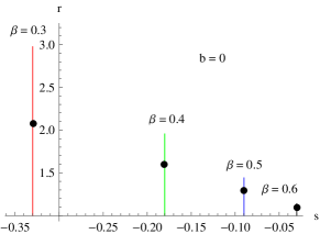
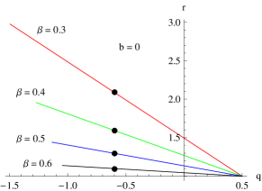
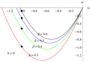
Figure 1: (Color online.) The curves of $r(s)$, $r(q)$ and $w^{\prime}(w)$ in the ERDE model without interaction respectively in the $r-s$, $r-q$ and $w^{\prime}-w$ planes for variable $\beta$. The dots denote today’s values of these parameters and $q_{0}=-0.595$ and $w_{0}=-1$ for all the cases.

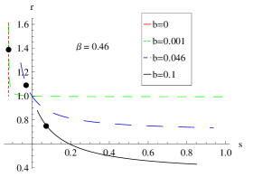
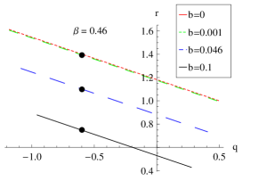
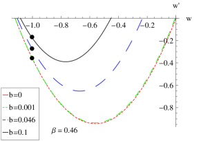
Figure 2: (Color online.) The curves of $r(s)$, $r(q)$ and $w^{\prime}(w)$ in the ERDE model with interaction respectively in the $r-s$, $r-q$ and $w^{\prime}-w$ planes for variable $b$ with the best-fit $\beta=0.46$. The dots denote today’s values of these parameters and $q_{0}=-0.595$ and $w_{0}=-1$ for all the cases.

In what follows, we do diagnosis with the statefinder to the above ERDE model. According to one of the basic dynamical equations of cosmology

$$\frac{\ddot{a}}{a}=-\frac{4\pi G}{3}(\rho+3p),$$ (15)

where $\rho$ and $p$ denote respectively the total energy density and pressure of the universe, the statefinder parameters have the form in terms of $\rho$ and $p$,

$$r=1+\frac{9(\rho+p)}{2\rho}\frac{\dot{p}}{\dot{\rho}},\ \ \ s=\frac{(\rho+p)}{p}\frac{\dot{p}}{\dot{\rho}},$$ (16)

as well as the deceleration parameter

$$q=-\frac{\ddot{a}}{aH^{2}}=\frac{1}{2}+\frac{3p}{2\rho}.$$ (17)

Further, in view of $\rho=\rho_{m}+\rho_{de}$ and $p=p_{m}+p_{de}=p_{de}=w\rho_{de}$, $\rho$ keeps conserved and satisfies $\dot{\rho}=-3H(\rho+p)$ while $\dot{p}=\dot{w}\rho_{de}+w\dot{\rho}_{de}$. Note that the conservation equation of dark energy (4) is a little more complicated, so we introduce the effective equation of state of dark energy by

$$w^{\textrm{eff}}=w+b(1+r_{\rho}),$$ (18)

then Eq. (4) recovers the standard form

$$\dot{\rho}_{de}+3H(1+w^{\textrm{eff}})\rho_{de}=0.$$ (19)

So the statefinder and deceleration parameters can be expressed as

$$r = 1-\frac{3}{2}\Omega_{de}\left[w^{\prime}-3w(1+w^{\textrm{eff}})\right],$$ (20)

$$s = 1+w^{\textrm{eff}}-\frac{w^{\prime}}{3w},$$ (21)

$$q = \frac{1}{2}+\frac{3}{2}w\Omega_{de},$$ (22)

where “ ^′ ” denotes the derivative with respect to $x=\ln a$ and $H=dx/dt$. When there is no interaction, i.e., $b=0$, we have $w^{\rm eff}=w$. Therefore, the LCDM model with $w=-1$ leads to constant statefinder parameters below

$$\{r,s\}|_{\rm LCDM}=\{1,0\}.$$ (23)

This means that the LCDM model corresponds to a fixed point $(s=0,r=1)$ in the statefinder $r-s$ plane. Thus, in virtue of this feature, other models of dark energy can be measured for the distance between them and the LCDM point to study their behaviors.

First, we plot curves of $r(s)$, $r(q)$ and $w^{\prime}(w)$ in the ERDE model without interaction respectively in the $r-s$, $r-q$ and $w^{\prime}-w$ planes in Fig. 1. In the $r-s$ plane, we see clearly that $r$ is time dependent while $s$ constant. This is the same as that in quiessence models (QCDM) in which $w={\rm constant}\neq-1$. But what’s different is shown in the $w^{\prime}-w$ plane, i.e., $w$ is not a constant. Especially when $\alpha=2\beta$, the model reduces to RDE. The trajectories of statefinder parameters coincide with that in Ref. [47], namely, $\beta=0.5$ makes the statefinder pair $\{r,s\}$ a fixed point $\{1,0\}$ corresponding to LCDM model and the universe ends in a de Sitter phase corresponding to the point $(w=-1,w^{\prime}=0)$ in the $w^{\prime}-w$ plane, also if $\beta<0.5$, the trajectories will lie in the region $r>1$, $s<0$ while $\beta>0.5$ in the region $r<1$, $s>0$. This is sort of different from the general case (1), in which $r$ starts from $1$ to increase and $s<0$ for the fitting $\beta$, even for $\beta>0.5$. Therefore it is concluded that in the non-interacting case the model does not reach the LCDM point $\{1,0\}$.

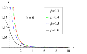
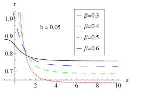
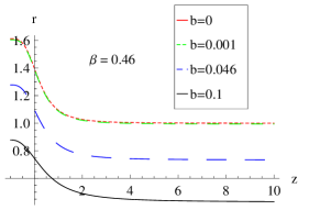
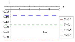
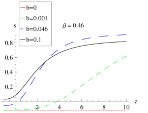
Figure 3: (Color online.) The evolutions of the statefinder parameters $r$ and $s$ with respect to the redshift $z$ in the ERDE model without and with interaction.

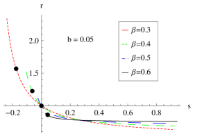
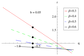
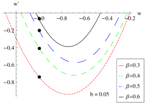
Figure 4: (Color online.) The curves of $r(s)$, $r(q)$ and $w^{\prime}(w)$ in the ERDE model with interaction respectively in the $r-s$, $r-q$ and $w^{\prime}-w$ planes for variable $\beta$ with $b=0.05$. The dots denote today’s values of these parameters and $q_{0}=-0.595$ and $w_{0}=-1$ for all the cases.

Secondly, let us see the effect of the interaction on the ERDE model from Fig. 2, where the best-fit values for parameters are taken [25, 47, 48, 51, 52, 53, 54]. In the $r-s$ plane, the interaction makes curves of $r(s)$ different essentially. The curves for interacting cases can reach or tend to the LCDM point $\{1,0\}$, even for very small $b$, and that both $r$ and $s$ are time dependent. Also the trajectories can lie in the region $r<1$ and $s>0$, which are forbidden in the non-interacting case (see the $r-s$ plane in Fig. 1). For the reason why this phenomenon appears, we can see it from the evolutions of $r$ and $s$ with respect to the redshift $z$ in the ERDE model without and with interaction in Fig. 3. Clearly the interaction can make $r$ cross $r=1$ and $s$ cross $s=0$, so curves of $r(s)$ can reach or tend to the LCDM point $\{1,0\}$, namely, the ranges of $r$ and $s$ are enlarged.

Finally, we plot curves of $r(s)$, $r(q)$ and $w^{\prime}(w)$ in the general HDE model with $b=0.05$ respectively in the $r-s$, $r-q$ and $w^{\prime}-w$ planes in Fig. 4. We find that for the case of $\beta=0.5$ and $b=0.05$, the statefinder pair $\{r,s\}$ evolves just at the LCDM point $\{1,0\}$ at present, as also can be recognized in Fig. 3, i.e., when $z\sim 0$, $r_{0}\sim 1$ and $s_{0}\sim 0$. Furthermore, we find that the smaller $\beta$ or $b$ is, the earlier the interacting model reaches the LCDM point $\{1,0\}$ in the $r-s$ plane. So for the ERDE model, the introduction of interaction makes its behavior more like other HDE models put forth before. That is to say, the ERDE model with interaction is more favored.

IV Conclusion

In this paper, we apply the statefinder diagnostic to the ERDE model without and with interaction. In the non-interacting case, $r$ is dependent of time while $s$ is a constant, like the QCDM models. But the difference between them is that $w$ is time dependent in the former while $w$ a constant in the latter. The non-interacting model does not reach the LCDM point $\{1,0\}$ in the $r-s$ plane. Especially for the case of $\alpha=2\beta$, it reduces to Ricci dark energy and $\beta=0.5$ plays an important role in its evolution [47]. In the interacting case, the interaction changes in essence the behavior of the ERDE model, because it makes $s$ no longer a constant and enlarges the ranges of $r$ and $s$, then the LCDM point can be reached or tended to. This is similar to other HDE models, so we can conclude that the ERDE model with interaction is more favored. We hope that the future high-precision observations can offer more and more accurate data to determine these parameters precisely and consequently shed light on the essence of dark energy.

- [1] A. G. Riess et al., Supernova Search Team Collaboration, Astron. J. 116 (1998) 1009.
- [2] S. Perlmutter et al., Supernova Cosmology Project Collaboration, Astrophys. J. 517 (1999) 565.
- [3] D. N. Spergel et al., WMAP Collaboration, Astrophys. J. Suppl. 148 (2003) 175.
- [4] D. N. Spergel et al., WMAP Collaboration, Astrophys. J. Suppl. 170 (2007) 377.
- [5] J. K. Adelman-McCarthy et al., SDSS Collaboration, Astrophys. J. Suppl. 175 (2008) 297.
- [6] R. A. Knop et al., Supernova Cosmology Project Collaboration, Astrophys. J. 598 (2003) 102.
- [7] E. Komatsu et al., WMAP Collaboration, Astrophys. J. Suppl. 180 (2009) 330.
- [8] V. Sahni and A. A. Starobinsky, Int. J. Mod. Phys. D 9 (2000) 373.
- [9] P. J. E. Peebles and B. Ratra, Rev. Mod. Phys. 75 (2003) 559.
- [10] E. J. Copeland, M. Sami, and S. Tsujikawa, Int. J. Mod. Phys. D 15 (2006) 1753.
- [11] M. Li, X. -D. Li, S. Wang, and Y. Wang, Commun. Theor. Phys. 56 (2011) 525.
- [12] T. P. Sotiriou and V. Faraoni, Rev. Mod. Phys. 82 (2010) 451.
- [13] S. Weinberg, Rev. Mod. Phys. 61 (1989) 1.
- [14] I. Zlatev, L. Wang, and P. J. Steinhardt, Phys. Rev. Lett. 82 (1999) 896.
- [15] R. R. Caldwell, Phys. Lett. B 545 (2002) 23.
- [16] B. Feng, X. Wang, and X. Zhang, Phys. Lett. B 607 (2005) 35.
- [17] T. Padmanabhan, Phys. Rev. D 66 (2002) 021301.
- [18] F. Piazza and S. Tsujikawa, J. Cosmol. Astropart. Phys. 07 (2004) 004.
- [19] G. ’t Hooft, arXiv:gr-qc/9310026.
- [20] A. Cohen, D. Kaplan, and A. Nelson, Phys. Rev. Lett. 82 (1999) 4971.
- [21] S. D. H. Hsu, Phys. Lett. B 594 (2004) 13.
- [22] M. Li, Phys. Lett. B 603 (2004) 1.
- [23] R. G. Cai, Phys. Lett. B 657 (2007) 228.
- [24] H. Wei and R. -G. Cai, Phys. Lett. B 660 (2008) 113.
- [25] C. Gao, F. Wu, X. Chen, and Y. -G. Shen, Phys. Rev. D 79 (2009) 043511.
- [26] L. N. Granda and A. Oliveros, Phys. Lett. B 669 (2008) 275.
- [27] V. Sahni, T. D. Saini, A. A. Starobinsky, and U. Alam, JETP Lett. 77 (2003) 201.
- [28] U. Alam, V. Sahni, T. D. Saini, and A. A. Starobinsky, Mon. Not. Roy. Astron. Soc. 344 (2003) 1057.
- [29] W. Zimdahl and D. Pavón, Gen. Rel. Grav. 36 (2004) 1483.
- [30] X. Zhang, Phys. Lett. B 611 (2005) 1.
- [31] X. Zhang, Commun. Theor. Phys. 44 (2005) 762.
- [32] P. Wu and H. Yu, Int. J. Mod. Phys. D 14 (2005) 1873.
- [33] X. Zhang, Commun. Theor. Phys. 44 (2005) 573.
- [34] X. Zhang, F. Q. Wu, and J. F. Zhang, J. Cosmol. Astropart. Phys. 01 (2006) 003.
- [35] H. Wei and R. -G. Cai, Phys. Lett. B 655 (2007) 1.
- [36] B. Chang, H. Liu, L. Xu, C. Zhang, and Y. Ping, J. Cosmol. Astropart. Phys. 01 (2007) 016.
- [37] B. Chang, H. Liu, L. Xu, and C. Zhang, Mod. Phys. Lett. A 23 (2008) 269.
- [38] Y. Shao and Y. Gui, Mod. Phys. Lett. A 23 (2008) 65.
- [39] Z. G. Huang, X. M. Song, H. Q. Lu, and W. Fang, Astrophys. Space Sci. 315 (2008) 175.
- [40] G. Panotopoulos, Nucl. Phys. B 796 (2008) 66.
- [41] A. Shojai and F. Shojai, Europhys. Lett. 88 (2009) 30002.
- [42] M. L. Tong and Y. Zhang, Phys. Rev. D 80 (2009) 023503.
- [43] L. Zhang, J. Cui, J. Zhang, and X. Zhang, Int. J. Mod. Phys. D 19 (2010) 21.
- [44] X. Zhang, Int. J. Mod. Phys. D 14 (2005) 1597.
- [45] M. R. Setare, J. Zhang, and X. Zhang, J. Cosmol. Astropart. Phys. 03 (2007) 007.
- [46] J. Zhang, X. Zhang, and H. Liu, Phys. Lett. B 659 (2008) 26.
- [47] C. -J. Feng, Phys. Lett. B 670 (2008) 231.
- [48] F. Yu, J. Zhang, J. Lu, W. Wang, and Y. Gui, Phys. Lett. B 688 (2010) 263.
- [49] M. Li, X. -D. Li, S. Wang, Y. Wang, and X. Zhang, J. Cosmol. Astropart. Phys. 12 (2009) 014.
- [50] E. Komatsu et al., Astrophys. J. Suppl. 192 (2011) 18.
- [51] X. Zhang, Phys. Rev. D 79 (2009) 103509.
- [52] M. Suwa and T. Nihei, Phys. Rev. D 81 (2010) 023519.
- [53] J. Zhang, L. Zhang, and X. Zhang, Phys. Lett. B 691 (2010) 11.
- [54] T. -F. Fu, J. -F. Zhang, J. -Q. Chen, and X. Zhang, Eur. Phys. J. C 72 (2012) 1932.