An Exactly Solvable Discrete Stochastic Process with Correlated Properties

Abstract

We propose a correlated stochastic process of which the novel non-Gaussian probability mass function is constructed by exactly solving moment generating function. The calculation of cumulants and auto-correlation shows that the process is convergent and scale invariant in the large but finite number limit. We demonstrate that the model consistently explains both the distribution and the correlation of discrete financial time-series data, and predicts the data distribution with high precision in the small number regime.

Non-normal distributions and time-series clustering are prevalent in physical and biological phenomena, such as in crystal growth, polymer transportation/distributionSornette ; deGennes , and brain electrical activityLehnertzEglger . In addition, non-normal distributions with high kurtosis (heavy-tail or leptokurtosis) and volatility clustering are frequently observed in the social science, such as in financial time-series dataKleinert ; Rachev and social networksBarabasi  . Leptokurtic distributions have been modeled by a family of stable distributions, constructed from the composite of independent and nonidentical Brownian and Poisson-jump processes. Clustering in time-series events is caused by the correlations between these events, for which various continuous and discrete models have been proposed to explain their phenomena. Auto-regressive moving average modelsRachev are popular continuous Gaussian stochastic models with correlated properties. Fractional Brownian motionMandelbrot is a continuous stochastic process, whose model is defined by the exponent of the power-law auto-correlation function of two white noises at different times. There are also various discrete models of correlated random walks, collectively referred to as urn models. Classical urn schemes are Polya’s modelPolyaUrn , which is implied by the $\beta$-distribution, and Friedman’s modelFriedmanUrn , which is a kind of dual to the Polya’s model. However, not much attention has been given to urn models in the analysis of time-series events, compared to the use of various continuous volatility models. Due to the inflexibility and limitations of current stochastic modelings, there is no unified prescription for the analysis of all kinds of data, and only few discrete processes are solved analytically. In such circumstances, it is worth developing a new discrete stochastic scheme constructed from a discrete micro process to explain the volatility of time-series data using correlations.

Figure 1: Ensemble paths of two iterations($N=2$), when $\kappa={1/2}$. A hollow circle represents half of the total initial number of white balls and a solid circle represents the same number of black balls. For example, the drawing of a white ball (upward right direction) increases the stochastic position by $+1$ and leads to the replacement of half of the black balls into white balls. One then proceeds to the next iteration.

In this Letter, we propose a binomial process of Markovian correlation. It is an urn model of ball replacement with a finite number of balls $\mathcal{N}$ and iterations $N$, which starts to converge at a large but finite number of iterations $N$. The process begins with the same $\mathcal{N}$ number of black and white balls in the urn, assuming unskewedness. In Ehrenfest’s urn scheme, one changes the color of a white ball to black in the case of drawing a black ball. After one round of drawing a black ball, one has $\mathcal{N}+1$ black balls and $\mathcal{N}-1$ white balls in the urn, and the probability of drawing a black ball in the second round turns to be biased as $1/2+1/2\mathcal{N}$. However, the process soon becomes ill-defined for $N$ iterations larger than $\mathcal{N}$. Therefore, Ehrenfest’s urn process is well-defined only for an infinite number of balls and iterations, solved by taking $N\rightarrow\infty$ limit, and convergent to the Ornstein-Uhlenbeck distribution in the continuum limitPolyaUrn . We generalize this process by adjusting the amount of color interchange throughout the whole process to make the process well-defined without taking $N\rightarrow\infty$ limit. Given the number of total iterations $N$, the ratio of interchange is adjusted to $2\kappa/N$ of the initial number of white/black balls $\mathcal{N}$, where $\kappa$ is the correlation parameter ranging from $-1/2$ to $1/2$. Thus, the probability of drawing a black ball after the aforementioned first round is generalized as $1/2+(\mathcal{N}\cdot 2\kappa/N)/2\mathcal{N}$. The rescaled correlation parameter is denoted as $\epsilon(N)={\kappa/N}$ for brevity. The stochastic displacement $\delta x_{n}$ at the time $n$ is either $+1$ or $-1$ depending on the outcome of white or black respectively, and the stochastic position $x_{n}$ at the $n$th iteration is defined by the difference between the historical outcomes of the white balls and that of the black balls (Fig. 1).

Within a few hundred iterations, this process describes the conspicuous non-Gaussian properties of finite $N$ statistics. Herein, we demonstrate the utility of our model in this regime by testing it on high-frequency financial time-series data, where the large volatility and positive auto-correlation are observed as its non-Gaussian entities. As $N$ grows larger, the process becomes scale invariant so that the cumulants start to converge. In the continuum limit, the proposed process ultimately converges to the Ornstein-Uhlenbeck distribution.

The recursion for the probability mass function(PMF) $P_{x,n}$ with the modified binomial transition probability is given as

$$\!\!P_{x,n\!+\!1}\!=\!P_{x\!+\!1,n}[{1\over 2}\!-\!{(x\!+\!1)}{\epsilon}]\!+\!P_{x\!-\!1,n}[{1\over 2}\!+\!{(x\!-\!1)}{\epsilon}]\,,$$ (1)

where $n=\{0,1,2,\cdots,N\}$  and each event is indexed as $n$ for the entire $N$ events. We define the stochastic location $x_{n}$ at the time $n$ by the accumulation of the stochastic displacements $\delta x_{i}$ of values $\pm 1$ from the origin, i.e. $x_{n}=\sum^{n}_{i=1}\delta x_{i}$ , and $x_{0}=0$. The location $x_{n}$ realized at the time after $n$ runs from $-n$ to $n$ in steps of $2$, i.e. $x_{n}\!\in\!\{-n\,,-n\!+\!2\,,-n\!+\!4\,,\cdots\,,n\!-\!2\,,n\}$, and the process starts with $P_{0,0}=1$. We omit the subscript $n$ on $x_{n}$, when the meaning is obvious. The process is the first order Markovian and becomes the Ornstein-Uhlenbeck equation with the density function $p(x,t)$ in the continuous limits of position and time: $\partial_{t}p=-2\epsilon\partial_{x}(xp)+{1/2}\partial_{x}^{2}p$.

The moment generating function is introduced as $Z_{n}(q)={\sum}_{x}q^{x}P_{x,n}\,,$ where $Z_{n}(0)={\sum}_{x}P_{x,n}=1$ . The moment generating function at time $0$ is defined as $Z_{0}(q)=1$, and then the recurrence in Eq. (1) is recast into a differential equation for $q$, shown as

$$Z_{n+1}(q)={1\over 2}(q+q^{-1})Z_{n}(q)+{\epsilon}(q^{2}-1)\partial_{q}Z_{n}(q)\,.$$ (2)

The substitution of $Z_{n}(q)=\epsilon^{n}(q-q^{-1})^{-{1/2\epsilon}}Y_{n}(q)$, leads to the simple equation

$$Y_{n+1}(q)=(q^{2}-1)\partial_{q}Y_{n}(q)\,$$ (3)

with $Y_{0}(q)=(q-q^{-1})^{1/2\epsilon}$ . A variable change of $q=-\tanh(r)$  gives the simpler equation, $Y_{n+1}(r)=\partial_{r}Y_{n}(r)$ with $Y_{0}(r)=[{\sinh(2r)/2}]^{-{1/2\epsilon}}$. Then, the partition function $Z_{n}(r)$ in the $r$ coordinate is

$$Z_{n}(r)=\epsilon^{n}\Big{[}\frac{\sinh(2r)}{2}\Big{]}^{\frac{1}{2\epsilon}}\partial_{r}^{n}\Big{[}\frac{\sinh(2r)}{2}\Big{]}^{-\frac{1}{2\epsilon}}.$$ (4)

Using the identity $\partial_{r}^{n}\sinh^{\alpha}(y)=\alpha{{-\alpha+n}\choose n}\sum_{k=1}^{n}(-1)^{k}(\alpha-k)^{-1}\sinh^{\alpha-k}(y)\partial_{y}^{n}\sinh^{k}(y)$, the closed form of the generating function is obtained as

$$\!\!\!\!\!\!\!\!\!\!\!\!\!\!\!Z_{n}(q)=\sum_{k=1}^{n}\sum_{i=0}^{k}{{{1/2\epsilon}+n}\choose{n}}{{n}\choose{k}}{{k}\choose{i}}\frac{(2\epsilon)^{n-1}(2i-k)^{n}}{({1/2\epsilon}+k)}\Big{[}-\frac{(1+q)^{2}}{4q}\Big{]}^{k}\Big{[}-\frac{(1-q)^{2}}{(1+q)^{2}}\Big{]}^{i}\,,$$ (5)

where the binomial function is defined as the product ${{{1/2\epsilon}+n}\choose{n}}={\prod_{i=0}^{n-1}({1/2\epsilon}+n-i)/n!}$. The Gaussian model is recovered with the absence of correlation, and therefore Eq. (5) becomes the familiar moment generating function of Bernoulli process; $\displaystyle\lim_{\epsilon\to 0}Z_{n}(q)={1/2^{n}}(q+q^{-1})^{n}\,.$ Cumulants are calculated from the derivatives of the generating function Eq. (5) . As expected, the average and the skewness are both zero. The variance and the fourth moment at the final time $N$, in the limit of small $\kappa$, are calculated to be

$$\!\!\!\!\!\!\langle x_{N}^{2}\rangle\!\!\!\! = \!\!\!\![\partial_{q}^{2}Z_{N}+\partial_{q}Z_{N}]|_{q=1}$$ (6)

$$= \!\!\!\!N\!\!+\!\!{4N\!(N\!\!-\!\!1)\over 2!}{\kappa\over N}\!\!+\!\!{{16}N\!(N\!\!-\!\!1)\!(N\!\!-\!\!2)\over 3!}\!(\!{\kappa\over N}\!)^{2}\!\!+\mathcal{\!O}(\!\kappa^{3}\!),\!\!$$

$$\!\!\!\!\!\!\langle x_{N}^{4}\rangle\!\!\!\! = \!\!\!\![\partial_{q}^{4}Z_{N}+6\partial_{q}^{3}Z_{N}+7\partial_{q}^{2}Z_{N}+\partial_{q}Z_{N}]|_{q=1}$$ (7)

$$= \!\!\!\!N(3N-2)+{8N(N\!\!-\!\!1)\over 2!}(3N\!\!-\!\!4){\kappa\over N}$$

$$\!\!\!\!+{56N(N\!\!-\!\!1)(N\!\!-\!\!2)\over 3!}(3N\!\!-\!\!{43\over 7})({\kappa\over N})^{2}+\mathcal{\!O}(\!\kappa^{3}\!).$$

Next, we directly iterate the stochastic process in Eq. (1) to compute the variance, fourth moment, and kurtosis of the PMF with positive and negative correlations with time (Fig. 2). They all grow non-linearly within several hundred iterations. The stochastic model in the small $N$ regime is used to explain positive correlations in financial time-series data, the details of which are discussed later in the text.

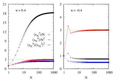
Figure 2: (Color online) Variance (square, blue), the fourth moment (triangle, black) and kurtosis (circle, red) as a function of $N$ with $\kappa=0.4$ (left) and $\kappa=-0.4$ (right). A guide line (y=3, green) is drawn as a reference.

In the large $N$ regime, the $i$th cumulants scaled by $N^{i/2}$ are independent of the number of iterations $N$ but only dependent on $\kappa$. Thus, $\kappa$ is the characteristic parameter to determine the PMF profile and there exists a scale invariance. They are shown to converge up to the second order of $\kappa$ in Eqs. (6) and (7), and we resort to numerical simulations for the higher order verification (Fig. 2). When the number of iterations is large ($10^{3}\mathchar 13358\relax N$), the variance grows linearly with $N$ and it is rewritten as $\langle x^{2}_{N}\rangle\!=\!H^{2}N$, where $H^{2}\equiv 1+2\kappa+8\kappa^{2}{/3}+\mathcal{O}(\kappa^{3})$ . In the Gaussian limit ($\kappa=0$), the diffusion speed is $H=1$ . For $\kappa>0$, where the stochastic process is positively correlated, $H>1$ and the process diffuses faster than the Brownian motion, whereas for $\kappa<0$, where the process is negatively correlated, $H<1$ and the process is less diffusive. The diffusion speed $H$, calculated from the Eq. (6) up to the order of $\kappa^{2}$ at the large $N$ regime, are $2.23$ for $\kappa=0.4$ and $0.63$ for $\kappa=-0.4$ , which are consistent with the numerical results in Fig. 3. In the calculation of kurtosis, nontrivial cancellations occur at each coefficient of $\kappa$ and $\kappa^{2}$, and consequently the quantity converges to $3$.

$$\lim_{N\to\infty}{\langle x_{N}^{4}\rangle\over\langle x_{N}^{2}\rangle^{2}}=3+\mathcal{O}(\kappa^{3})\,.$$ (8)

The numerically measured kurtosis in Fig.3 also confirms the convergence to $3$ at all orders of $\kappa$, which strongly corroborates the analytic result in Eq. (8).

The auto-correlation between tick displacements ($\delta x_{i}=\pm 1$) at time $n$ and time $n+l$ with a generic time lag $l=\{1\,,2\,,\cdots\}$ can be approximated as $\langle\delta x_{n}\delta x_{n+l}\rangle$ = ${2\kappa/N}+(H^{2}n+l-1)({2\kappa/N})^{2}+\mathcal{O}({1/N^{3}})$. At the large $N$ regime, the auto-correlation is renormalized as the order of $1/N$ in the same way as the rescaling of correlation $\epsilon=\kappa/N$, which again verifies the scale invariance. In addition, it is independent of the time parameter $n$, therefore the auto-correlation of tick displacements is stationary.

We test the model on high-frequency financial time-series datadata (Fig. 3A). Instead of the commonly used return statisticsKleinert ; Rachev , we directly employ discrete time-series statistics of tick movements. The collection of $N$ consecutive tick movements is assumed as a statistical ensemble so that it corresponds to $x_{N}$(Fig. 3B,C). The distribution of such ensemble data $P(x)$, where $x=x_{N}$ is the sum of $N$ consecutive tick displacements $\delta x=\pm 1$, has a characteristic profile with large volatility(Fig. 4A). Furthermore, positive correlation is observed(Fig. 4B). It is possible to relate the correlation between tick movements to the non-Gaussian profile of the data, since the PMF profile of the data is clearly different from the Bernoulli process where consecutive events are independent. Therefore, we examine whether the PMF $P(x|\epsilon,M)$ of our model $M$ with the correlation parameter $\epsilon(N)=\kappa/N$ can generate the ${P}(x)\pm\delta P(x)$ of the data. The discrepancy between the model and the data is defined as

$$E(\epsilon)=\sum_{x}\frac{[{P}(x)-P(x|\epsilon,M)]^{2}}{2\delta^{2}{P}(x)}.$$ (9)

Given the mean $P(x)$ and uncertainty $\pm\delta P(x)$ of the data $D$, the model likelihood becomes $P(D|\epsilon,M)\propto\exp[-E(\epsilon)]$ due to the maximal entropy principleSivia . Using a uniform prior assumption, about the parameter $\epsilon$, i.e. $P(\epsilon|M)$=constant, the posterior probability of $\epsilon$ given data $D$ can be written as

$$P(\epsilon|D,M)=P(\epsilon|M)\frac{P(D|\epsilon,M)}{P(D|M)}=\frac{\exp[-E(\epsilon)]}{\int d\epsilon\exp[-E(\epsilon)]}$$ (10)

by the product rule in probability theory. Then, it is straightforward to compute the expectation value $\langle\epsilon\rangle=\int d\epsilon\,\epsilon\,P(\epsilon|D,M)$ and its uncertainty $\delta\epsilon=[\int d\epsilon\,\epsilon^{2}\,P(\epsilon|D,M)-\langle\epsilon\rangle^{2}]^{1/2}$. We estimate the correlation parameter from the financial data using Markov Chain Monte-Carlo (MCMC) methodGregory with $10^{5}$ MC steps after equilibration: $\epsilon(10)=0.0475\pm 0.0003$, $\epsilon(20)=0.0229\pm 0.0001$, and $\epsilon(30)=0.0154\pm 0.0000(5)$ for $N$=10, 20, and 30, respectively. However, the corresponding values of the correlation parameter $\kappa=\epsilon N$ are similar to each other (0.48, 0.46, and 0.46, repeatedly) which confirms the robustness of the obtained data distribution (Fig. 4A).

Figure 3: (A) Standard $\&$ Poors futures prices of all transaction recordsdata $s_{t}$, where $t$ indicates each transaction event. (B) The data enlarged over a short period. (C) Tick movement decomposed from the time-series data of (B). The minimum tick movement is set as $\pm 1$ by rescaling the minimum tick size $\pm 0.1$. The integer-valued time-series from the raw data is denoted as $\{s_{1},s_{2},\cdots,s_{t},\cdots\}$, and the time-series difference is denoted as $\{s_{2}-s_{1},s_{3}-s_{2},\cdots,s_{t+1}-s_{t},\cdots\}$. We decompose the time-series of differences into a series of $\pm 1$ of the length $|s_{t+1}-s_{t}|$, depending on the sign of $s_{t+1}-s_{t}$. For example, the time-series $\cdots 1463.7,1463.9,1464.0,1463.8,\cdots$ is mapped into the tick movements $\cdots(+1,+1),+1,(-1,-1),\cdots$ in our analysis.

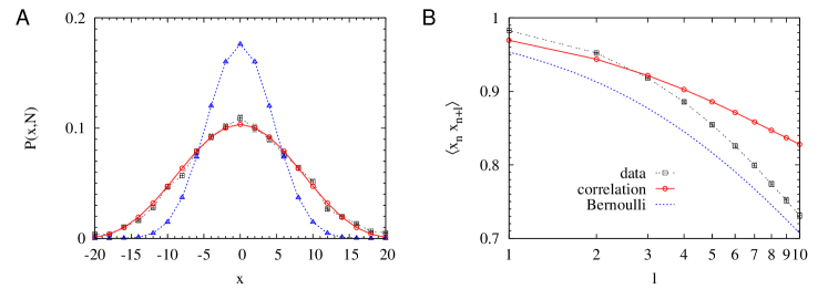
Figure 4: (Color online) Frequency and auto-correlation plots of our financial data. (A) Frequency of cumulative tick movement for $N=20$ consecutive times and (B) auto-correlation between $n=10$ and $n+l$ consecutive tick movements with $l=\{1,2,...,10\}$; financial data (square, black); Bernoulli process in the absence of correlation between events (triangle, blue); correlation model with $\kappa=0.45$ (circle, red). For both plots, we used $10^{4}$ samples of $x=x_{N}$ for (A) frequency and also $10^{4}$ samples of $x_{n}x_{n+l}$ from the financial tick series. For their uncertainty estimation, we used 100 ensembles of the given $10^{4}$ samples. Note that data uncertainty (standard deviation) is smaller than the symbol size. The auto-correlation for the Bernoulli process is $\sqrt{(n/n+l)}$.

In the model, we also calculate the auto-correlation between the stochastic positions $x_{n}$ and $x_{n+l}$ with time lag $l$ as

$${\langle x_{n}x_{n+l}\rangle\over\sqrt{\langle x_{n}^{2}\rangle\langle x_{n+l}^{2}\rangle}}=\sqrt{\!{\langle x_{n}^{2}\rangle}\over{\langle x_{n+l}^{2}\rangle}}(1+2\epsilon)^{l}\,\,\,\xrightarrow{\!\kappa=0\!}\sqrt{n\over n+l},$$ (11)

which is abbreviated as $C(n,l|\epsilon,M)$ with the specification of $\epsilon$. The corresponding data correlation is measured from the random choices of consecutive $x_{n}$ and $x_{n+l}$ in the data, and it is denoted as $C(n,l)\pm\delta C(n,l)$ (Fig. 4B). From the correlation parameter $\kappa$ that is extracted from the histogram, we can independently estimate the correlation parameter $\kappa^{\prime}$ from the auto-correlation. For this reason, we also define the discrepancy between the model and the data as

$$E^{\prime}(\epsilon,n)=\sum_{l=1}^{L}\frac{[C(n,l)-C(n,l|\epsilon,M)]^{2}}{2\delta^{2}C(n,l)},$$ (12)

where the total iteration number is constrained as $N=n+L$. Following the previous procedures, we estimate the correlation parameter $\kappa^{\prime}$=0.43 ($n$=5, $L=15$), 0.41 ($n$=10, $L$=10), and 0.38 ($n=15$, $L=5$) in three cases satisfying the condition, $N=20$. The measured correlation $\kappa^{\prime}$ from the auto-correlation is close to the correlation $\kappa$ measured from the histogram. This approximated overlap between $\kappa$ and $\kappa^{\prime}$, extracted from two independent measurements, is remarkable. In Fig. 4B, the auto-correlation of data is matched well with the model for small time lag $l$, while the result is matched well with the Bernoulli process for large lag large $l$. In other words, the financial data show strong correlation between events with small time lag. However, after a certain finite time lag, the correlation becomes negligible so that the auto-correlation with sufficient time lag converges to the auto-correlation of the Bernoulli process. To compare which models explain the auto-correlation better within the finite lag window in Fig. 4B, we compute the Bayes factor between two models of our correlation model $M$ versus the Bernoulli model $B$:

$$\frac{P(D|M)}{P(D|B)}=\frac{\int d\epsilon P(D|\epsilon,M)P(\epsilon|M)}{P(D|\epsilon\!=\!0,M)}.$$ (13)

The Bayes factor, $\ln[P(D|M)/P(D|B)]\!\sim\!10^{4}$ demonstrates that the correlation model explains the auto-correlation result exceedingly better than the Bernoulli model in the absence of correlation between events.

Our proposed model offers a new scheme of volatility prediction based on the detection of correlations. Unlike ordinary continuous Gaussian volatility prediction models, such as auto-regressive moving average models and generalized auto-regressive conditional heteroskedasticity models, our model can explain finite $N$ statistics, and can predict real data with outstanding precision and high efficiency due to the analytic result.

- (1) D. Sornette, Critical Phenomena in Natural Sciences, Springer, Berlin, 2nd Ed. p.163., (2004).
- (2) P. de Gennes, Introduction to Polymer Dynamics, Cambridge University Press, Chap.1., (1992).
- (3) K. Lehnertz and C. Elger, Can epileptic seizures be predicted? Evidence from nonlinear time series analysis of brain electrical activity. Phys Rev Lett 80:5019–22, (1998)
- (4) Hagen Keinert , Path Integrals in Quantum Mechanics, Statistics, Polymer Physics, and Financial Markets, 5th Ed. p. 1432 , (2009).
- (5) Rachev, S.T. and Mittnik, S. Stable Paretian Models in Finance. New York: Jone Wiley Sons, (2000).
- (6) A.-L. Barabasi and R. Albert, Science 286, 509 (1999).
- (7) B. Mandelbrot, and J.W. van Ness, Fractional Brownian motions, fractional noises and applications, SIAM Review 10, (1968).
- (8) Norman L. Johnson and Samuel Kotz, Urn models and their application: an approach to modern discrete probability theory, Wiley, p. 176., (1977).
- (9) B. Friedman, A Simple Urn Model , Comm. Pure Appl. Math., (1949).
- (10) W. Feller, Introduction to Probability Theory and Its Applications, Wiley, (1968).
- (11) D.S. Sivia, Data analysis: A Bayesian tutorial, (2006)
- (12) P. Gregory, Bayesian logical data analysis for the physical sciences, (2010)
- (13) Standard Poor’s Futures prices between 2013.1.20 and 2013.3.18, received from Thomson Reuters machine. Data sets are offered by Byoung Ki Seo at Ulsan National Institute of Science and Technology.