Ferromagnetism and Fermi-surface transition in the periodic Anderson model: Second-order phase transition without symmetry breaking

Abstract

We study ferromagnetism in the periodic Anderson model with and without a magnetic field by the Gutzwiller theory. We find three ferromagnetic phases: a weak ferromagnetic phase (FM0), a half-metallic phase without Fermi surface for the majority spin (FM1), and a ferromagnetic phase with almost completely polarized $f$-electrons (FM2). The Fermi surface changes from the large Fermi-surface in the paramagnetic state to the small Fermi-surface in FM2. We also find that the transitions between the ferromagnetic phases can be second-order phase transitions in spite of the absence of symmetry breaking. While we cannot define an order parameter for such transitions in an ordinary way, the topology of the Fermi surface characterizes the transitions, i.e., they are Lifshitz transitions.

I Introduction

In heavy-fermion systems, external perturbations, such as a magnetic field $H$ and pressure, can change the electronic state drastically, since the energy scale in the heavy-fermion systems is very low due to the renormalization by the strong electron correlation.

The metamagnetic behavior in CeRu₂Si₂ Besnus et al. (1985); Haen et al. (1987); van der Meulen et al. (1991); Aoki et al. (1993) under a magnetic field and the magnetic field induced transitions in YbRh₂Si₂ Tokiwa et al. (2005); Rourke et al. (2008); Pfau et al. ; Pourret et al. (2013) are typical examples of such effects. At the transition field, the magnetization deviates substantially from a linear dependence on $H$ observed in lower fields. Besnus et al. (1985); Haen et al. (1987); Tokiwa et al. (2005) Such an anomaly in the magnetization indicates that the electronic state is changed drastically at the transition. Indeed, the effective mass deduced from the specific heat van der Meulen et al. (1991) and from the de Haas-van Alphen effect Aoki et al. (1993) enhances around the metamagnetic field in CeRu₂Si₂. In YbRh₂Si₂, change in the Fermi surface from the de Haas-van Alphen experiment Rourke et al. (2008) and anomaly in the thermoelectric power Pfau et al. ; Pourret et al. (2013) around 10 T have been reported.

Another examples are magnetic transitions and superconductivity under pressure, such as ferromagnetic transitions Pfleiderer and Huxley (2002) and superconductivity Saxena et al. (2000) in UGe₂. There are two ferromagnetic phases in UGe₂: the strongly polarized ferromagnetic phase phase under low pressure, called FM2, and the ferromagnetic phase under high pressure, called FM1. Under higher pressures, UGe₂ becomes paramagnetic. The superconducting transition temperature becomes maximum around the pressure where the FM1-FM2 transition temperature becomes zero. Tateiwa et al. (2001) The coefficient $A$ of $T^{2}$ term in the electrical resistivity, $\sqrt{A}$ is proportional to the effective mass, enhances in FM1. Oomi et al. (1998); Saxena et al. (2000); Tateiwa et al. (2001); Settai et al. (2002) The de Haas-van Alphen experiments show that the Fermi surface changes at the ferromagnetic transitions. Terashima et al. (2001); Settai et al. (2002); Terashima et al. (2002); Haga et al. (2002); Settai et al. (2003) These observations indicate that the electronic state changes drastically at the ferromagnetic transitions.

To understand such phenomena, we need a theory which can describe the heavy-fermion state and the magnetically polarized state, and can evaluate physical quantities which reflect the change in the electronic state, such as the effective mass. To describe the heavy-fermion state, the periodic Anderson model has been employed as a typical model. While several approximations have been applied to the model, the Gutzwiller method is a useful approximation and succeeded in describing the heavy-fermion state. Rice and Ueda (1986); Fazekas and Brandow (1987) Thus, it is natural to extend the Gutzwiller method for the model with magnetic polarization. In fact, a similar approximation, that is, the slave-boson mean-field theory of the Kotliar-Ruckenstein type, has been applied to study the magnetization of the model. Reynolds et al. (1992); Dorin and Schlottmann (1993a, b) However, the effects of magnetism and a magnetic field on the effective mass have not been explored by these studies.

In this study, we extend the Gutzwiller method for the magnetically polarized states, and investigate ferromagnetic states at zero temperature. We evaluate the magnetization and the effective mass. We also investigate the Fermi-surface change by ferromagnetism and a magnetic field. Preliminary results on the magnetic field effect have been reported in Ref. Kubo, 2013.

This paper is organized as follows. In Sec. II, we explain the periodic Anderson model. In Sec. III, we introduce the variational wave function and the Gutzwiller approximation. In Sec. IV, we show the calculated results of physical quantities and phase diagrams. We also discuss Fermi-surface states and the order of the phase transitions. In Sec. V, we discuss the antiferromagnetic states of the model. In Sec. VI, we summarize the paper.

II Model

The periodic Anderson model is given by

$$\begin{split}\mathcal{H}=&\sum_{\mathbf{k}\sigma}\epsilon_{\mathbf{k}}c^{\dagger}_{\mathbf{k}\sigma}c_{\mathbf{k}\sigma}+\sum_{i\sigma}\epsilon_{f}n_{fi\sigma}\\ -&V\sum_{\mathbf{k}\sigma}(f^{\dagger}_{\mathbf{k}\sigma}c_{\mathbf{k}\sigma}+c^{\dagger}_{\mathbf{k}\sigma}f_{\mathbf{k}\sigma})+U\sum_{i}n_{fi\uparrow}n_{fi\downarrow},\end{split}$$ (1)

where $c^{\dagger}_{\mathbf{k}\sigma}$ and $f^{\dagger}_{\mathbf{k}\sigma}$ are the creation operators of the conduction and $f$ electrons, respectively, with momentum $\mathbf{k}$ and spin $\sigma$. $n_{fi\sigma}$ is the number operator of the $f$ electron with spin $\sigma$ at site $i$. $\epsilon_{\mathbf{k}}$ is the kinetic energy of the conduction electron, $\epsilon_{f}$ is the $f$-electron level, $V$ is the hybridization matrix element, and $U$ is the onsite Coulomb interaction between $f$ electrons. The spatial extent of the $f$-electron wave-function is narrow and the Coulomb interaction between $f$ electrons is large, and thus, we set $U\rightarrow\infty$ for simplicity. We set the energy level of the conduction electrons as the origin of energy, that is, $\sum_{\mathbf{k}}\epsilon_{\mathbf{k}}=0$.

Under a finite magnetic field $H$, we replace $\epsilon_{f}$ by $\epsilon_{f\sigma}=\epsilon_{f}-\sigma H$, where $\sigma=+1$ ($-1$) for $\uparrow$ ($\downarrow$) spin in the right hand side of the equation. Here, we have set the Bohr magneton $\mu_{\text{B}}=1$ as the unit of magnetization. We have set the $g$-factors $g_{f}=2$ for $f$ electrons and $g_{c}=0$ for conduction electrons, that is, we ignore the Zeeman term for the conduction electrons. As we will show later, the polarization of the conduction electrons is small even in ferromagnetic phases, and this assumption is justified as long as the magnetic field is not very large.

Experimentally, magnetic anisotropy is important in $f$-electron systems, while it is not included in the present model. To interpret experimental results, we should regard the magnetization and magnetic field of the present theory as being along the easy axis of the materials.

III Method

In this study, we focus on ferromagnetism and magnetic field effects on the paramagnetic state, and then, we assume a spatially uniform state. The variational wave function is given by

$$|\psi\rangle=P|\phi_{\uparrow}\rangle\otimes|\phi_{\downarrow}\rangle,$$ (2)

where $P=\prod_{i}[1-n_{fi\uparrow}n_{fi\downarrow}]$ excludes the double occupancy of the $f$ electrons at the same site. For the one-electron part of the wave function, we consider the following form:

$$|\phi_{\sigma}\rangle=\prod_{k<k_{\mathrm{F}\sigma}}[c^{\dagger}_{\mathbf{k}\sigma}+a_{\sigma}(\mathbf{k})f^{\dagger}_{\mathbf{k}\sigma}]|0\rangle,$$ (3)

for $n_{\sigma}<1$, where $n_{\sigma}$ is the total number of the spin-$\sigma$ electrons per site and $k_{\mathrm{F}\sigma}$ is the Fermi momentum for spin $\sigma$. $a_{\sigma}(\mathbf{k})$ are spin-dependent variational parameters. For $n_{\sigma}>1$, both the hybridized bands are filled below $k_{\mathrm{F}\sigma}$ and only the lower hybridized band is filled above $k_{\mathrm{F}\sigma}$ for $U=0$, and thus, we consider the one-electron part given by

$$|\phi_{\sigma}\rangle=\prod_{p<k_{\mathrm{F}\sigma}}c^{\dagger}_{\mathbf{p}\sigma}f^{\dagger}_{\mathbf{p}\sigma}\prod_{k>k_{\mathrm{F}\sigma}}[c^{\dagger}_{\mathbf{k}\sigma}+a_{\sigma}(\mathbf{k})f^{\dagger}_{\mathbf{k}\sigma}]|0\rangle.$$ (4)

By using the Gutzwiller approximation, Fazekas and Brandow (1987); Kubo (2011a, b) we evaluate the expectation values of physical quantities of the variational wave function. The $f$-electron number $n_{f\sigma}$ per site with spin $\sigma$ is given by

$$n_{f\sigma}=\frac{1}{L}\sum_{k<k_{\text{F}\sigma}}\frac{a^{2}_{\sigma}(\mathbf{k})}{q^{-1}_{\sigma}+a^{2}_{\sigma}(\mathbf{k})},$$ (5)

for $n_{\sigma}<1$, and

$$n_{f\sigma}=\frac{1}{L}\sum_{k>k_{\text{F}\sigma}}\frac{a^{2}_{\sigma}(\mathbf{k})}{q^{-1}_{\sigma}+a^{2}_{\sigma}(\mathbf{k})}+n_{\sigma}-1,$$ (6)

for $n_{\sigma}>1$, where $L$ is the number of the lattice sites and

$$q_{\sigma}=\frac{1-n_{f}}{1-n_{f\sigma}},$$ (7)

with $n_{f}=\sum_{\sigma}n_{f\sigma}$. $n_{\sigma}-1$ in Eq. (6) is the $f$-electron number with spin $\sigma$ inside the Fermi momentum $k_{\text{F}\sigma}$.

We evaluate the momentum distribution functions $n_{c\sigma}(\mathbf{k})=\langle c^{\dagger}_{\mathbf{k}\sigma}c_{\mathbf{k}\sigma}\rangle=\langle\psi|c^{\dagger}_{\mathbf{k}\sigma}c_{\mathbf{k}\sigma}|\psi\rangle/\langle\psi|\psi\rangle$ of the conduction electrons and $n_{f\sigma}(\mathbf{k})=\langle f^{\dagger}_{\mathbf{k}\sigma}f_{\mathbf{k}\sigma}\rangle$ of the $f$ electrons. For $n_{\sigma}<1$, we obtain

$$n_{c\sigma}(\mathbf{k})=\begin{cases}\Delta n_{c\sigma}(\mathbf{k})&\text{for $k<k_{\text{F}\sigma}$}\\ 0&\text{for $k>k_{\text{F}\sigma}$}\end{cases},$$ (8)

with

$$\Delta n_{c\sigma}(\mathbf{k})=\frac{q^{-1}_{\sigma}}{q^{-1}_{\sigma}+a^{2}_{\sigma}(\mathbf{k})},$$ (9)

and

$$n_{f\sigma}(\mathbf{k})=\begin{cases}(1-q_{\sigma})n_{f\sigma}+\Delta n_{f\sigma}(\mathbf{k})&\text{for $k<k_{\text{F}\sigma}$}\\ (1-q_{\sigma})n_{f\sigma}&\text{for $k>k_{\text{F}\sigma}$}\end{cases},$$ (10)

with

$$\Delta n_{f\sigma}(\mathbf{k})=q_{\sigma}\frac{a^{2}_{\sigma}(\mathbf{k})}{q^{-1}_{\sigma}+a^{2}_{\sigma}(\mathbf{k})}.$$ (11)

For $n_{\sigma}>1$, we obtain

$$n_{c\sigma}(\mathbf{k})=\begin{cases}1&\text{for $k<k_{\text{F}\sigma}$}\\ 1-\Delta n_{c\sigma}(\mathbf{k})&\text{for $k>k_{\text{F}\sigma}$}\end{cases},$$ (12)

with

$$\Delta n_{c\sigma}(\mathbf{k})=\frac{a^{2}_{\sigma}(\mathbf{k})}{q^{-1}_{\sigma}+a^{2}_{\sigma}(\mathbf{k})},$$ (13)

and

$$n_{f\sigma}(\mathbf{k})=\begin{cases}q_{\sigma}+(1-q_{\sigma})n_{f\sigma}&\text{for $k<k_{\text{F}\sigma}$}\\ q_{\sigma}+(1-q_{\sigma})n_{f\sigma}-\Delta n_{f\sigma}(\mathbf{k})&\text{for $k>k_{\text{F}\sigma}$}\end{cases},$$ (14)

with

$$\Delta n_{f\sigma}(\mathbf{k})=q_{\sigma}\frac{q^{-1}_{\sigma}}{q^{-1}_{\sigma}+a^{2}_{\sigma}(\mathbf{k})}.$$ (15)

Energy per site is given by

$$e=\frac{\langle\mathcal{H}\rangle}{L}=\sum_{\sigma}e_{\sigma},$$ (16)

where

$$e_{\sigma}=\frac{1}{L}\sum_{k<k_{\text{F}\sigma}}\epsilon_{\mathbf{k}}+\frac{1}{L}\sum_{k<k_{\text{F}\sigma}}\frac{(\epsilon_{f\sigma}-\epsilon_{\mathbf{k}})a^{2}_{\sigma}(\mathbf{k})-2Va_{\sigma}(\mathbf{k})}{q^{-1}_{\sigma}+a^{2}_{\sigma}(\mathbf{k})},$$ (17)

for $n_{\sigma}<1$, and

$$e_{\sigma}=\epsilon_{f\sigma}(n_{\sigma}-1)+\frac{1}{L}\sum_{k>k_{\text{F}\sigma}}\frac{(\epsilon_{f\sigma}-\epsilon_{\mathbf{k}})a^{2}_{\sigma}(\mathbf{k})-2Va_{\sigma}(\mathbf{k})}{q^{-1}_{\sigma}+a^{2}_{\sigma}(\mathbf{k})},$$ (18)

for $n_{\sigma}>1$.

Now, we minimize the energy with respect to the variational parameters $a_{\sigma}(\mathbf{k})$. From $\partial e/\partial a_{\sigma}(\mathbf{k})=0$, we obtain

$$a_{\sigma}(\mathbf{k})=\frac{2V}{\tilde{\epsilon}_{f\sigma}-\epsilon_{\mathbf{k}}+\sqrt{(\tilde{\epsilon}_{f\sigma}-\epsilon_{\mathbf{k}})^{2}+4\tilde{V}^{2}_{\sigma}}},$$ (19)

where $\tilde{V}_{\sigma}=\sqrt{q_{\sigma}}V$ and $\tilde{\epsilon}_{f\sigma}$ is the renormalized $f$-level. The renormalized $f$-level $\tilde{\epsilon}_{f\sigma}$ satisfy

$$\epsilon_{f\sigma}-\tilde{\epsilon}_{f\sigma}=-\sum_{\sigma^{\prime}}\tilde{V}^{2}_{\sigma^{\prime}}I_{2\sigma^{\prime}}q_{\sigma^{\prime}}\frac{\partial q^{-1}_{\sigma^{\prime}}}{\partial n_{f\sigma}}.$$ (20)

The integral is defined by

$$I_{l\sigma}=\frac{1}{L}{\sum_{\mathbf{k}}}^{\prime}\frac{(\epsilon_{\mathbf{k}}-\tilde{\epsilon}_{f\sigma})^{l-2}}{\sqrt{(\epsilon_{\mathbf{k}}-\tilde{\epsilon}_{f\sigma})^{2}+4\tilde{V}^{2}_{\sigma}}},$$ (21)

where ${\sum_{\mathbf{k}}}^{\prime}$ means that the summation runs over $k<k_{\text{F}\sigma}$ for $n_{\sigma}<1$ and $k>k_{\text{F}\sigma}$ for $n_{\sigma}>1$. We can rewrite Eqs. (5) and (6) by using Eqs. (19) and (21):

$$n_{f\sigma}=\frac{n_{\sigma}+I_{3\sigma}}{2}.$$ (22)

We solve Eqs. (20) and (22) with respect to $\tilde{\epsilon}_{f\sigma}$ and $n_{f\sigma}$ for each value of the total polarization $M^{\prime}=n_{\uparrow}-n_{\downarrow}$ fixing the total number $n=n_{\uparrow}+n_{\downarrow}$ of electrons per site, and evaluate the energy. $n_{\sigma}$ can be tuned by varying the Fermi momentum $k_{\text{F}\sigma}$. Then, we determine $M^{\prime}$ for which the energy is the lowest, and evaluate physical quantities. Here, we note that Eqs. (20) and (22) can be derived also by the slave-boson mean-field theory of the Kotliar-Ruckenstein type, Dorin and Schlottmann (1993a) and several physical quantities, such as magnetism, are equivalent between the slave-boson mean-field theory and the Gutzwiller method. However, some quantities are difficult to be determined within the slave-boson mean-field theory. For example, for $n_{\sigma}<1$, the electron distribution function is always the Fermi distribution function, that is, unity below the Fermi momentum and zero above the Fermi momentum, since the slave-boson mean-field theory is a one-particle approximation. Thus, we obtain $\Delta n_{c\sigma}(k_{\text{F}\sigma})+\Delta n_{f\sigma}(k_{\text{F}\sigma})=1$. On the other hand, we can deal with the renormalization effect on the electron distribution by the Gutzwiller method as shown in Eqs. (8)–(15).

IV Results

Before presenting our calculated results, we discuss possible ferromagnetic states of the model by using schematic band structures shown in Fig. 1.

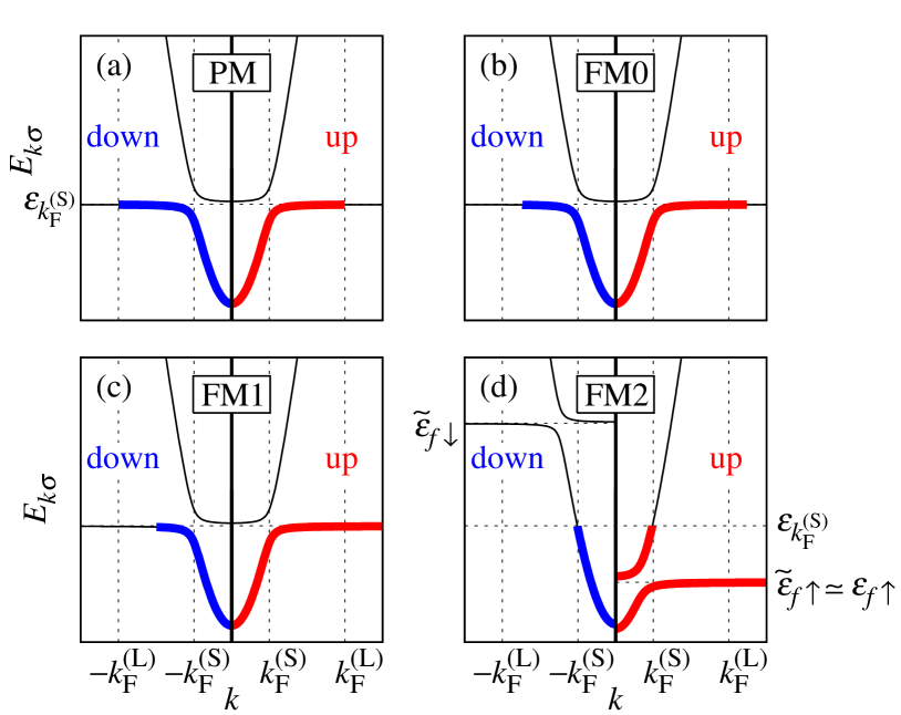
Figure 1: (Color online) Schematic band structures of paramagnetic and ferromagnetic phases in the periodic Anderson model. (a) paramagnetic phase (PM), (b) weakly polarized ferromagnetic phase (FM0), (c) half-metallic phase (FM1), and (d) ferromagnetic phase with an almost completely polarized $f$-electron state (FM2). $E_{k\sigma}$ denotes the quasi-particle energy. Right (left) part of each figure shows the up- (down-) spin band. The occupied states are represented by the bold lines.

In the paramagnetic phase (PM), Fig. 1(a), the numbers of up- and down-spin electrons are the same. The effective $f$-level $\tilde{\epsilon}_{f\uparrow}=\tilde{\epsilon}_{f\downarrow}$ is renormalized to a value around the kinetic energy $\epsilon_{k^{\text{(S)}}_{\text{F}}}$ at the Fermi momentum for the small Fermi-surface as long as $\epsilon_{f}\ll\epsilon_{k^{\text{(S)}}_{\text{F}}}$, and the Fermi level is also near $\epsilon_{k^{\text{(S)}}_{\text{F}}}$. Here, the small Fermi-surface is defined as the Fermi surface for the state where the $f$ orbital with $n_{f}=1$ is assumed to be decoupled from the conduction electrons. However, the $f$-electron state contributes to the band, and the large Fermi-surface realizes with the Fermi momentum $k^{\text{(L)}}_{\text{F}}$ which includes the $f$-electron contribution. As a result, the dispersion around Fermi momentum $k^{\text{(L)}}_{\text{F}}$ is weak, and a heavy-electron state realizes. Note that if $\epsilon_{f}\gg\epsilon_{k^{\text{(S)}}_{\text{F}}}$, the renormalization is weak and $\tilde{\epsilon}_{f\uparrow}=\tilde{\epsilon}_{f\downarrow}\simeq\epsilon_{f}$.

In a state with weak polarization, by a spontaneous phase transition or by a magnetic field, the band structure will become like Fig. 1(b). Here, we call this state FM0.

When the polarization becomes larger, the lower hybridized band will be filled up by the up-spin electrons as shown in Fig. 1(c). We call this state FM1. In this state, the Fermi surface for the up-spin states disappears, that is, this is a half-metallic state. There is a hybridization gap, and this state will be stable in some degree. This half-metallic state has been obtained by the slave-boson mean-field theory Reynolds et al. (1992); Dorin and Schlottmann (1993a, b) and in the Kondo lattice model. Yu. Irkhin and Katsnelson (1991); Watanabe (2000); Viola Kusminskiy et al. (2008); Beach and Assaad (2008); Peters et al. (2012); Bercx and Assaad (2012); Peters and Kawakami (2012)

When the polarization increases further, the up-spin electrons start to fill the upper hybridized band as in Fig. 1(d). We call this state FM2. In FM2, the $f$ electrons will polarize almost completely, that is, $n_{f\uparrow}\simeq 1$ and $n_{f\downarrow}\simeq 0$. Since $n_{f\downarrow}\simeq 0$, the up-spin electrons can move almost freely, and the effective $f$-level for up spin should be near the bare $f$-level. On the other hand, the down-spin electrons experience the Coulomb interaction strongly for $n_{f\uparrow}\simeq 1$, and the effective $f$-level for down spin becomes much higher than the Fermi level. As a result, the electronic state around the Fermi surface is composed mostly of the conduction-electron states, and the Fermi surface is similar to that expected for the small Fermi-surface state. Such a small Fermi-surface induced by ferromagnetism and/or magnetic field has been discussed in Refs. Miyake and Ikeda, 2006; Suzuki and Harima, 2010.

Now, we show the calculated results in the following subsections. In the present study, we consider a simple model for the conduction band. The density of states of the conduction electrons is given by $\rho(\epsilon)=1/(2W)$ for $|\epsilon|<W$ and $\rho(\epsilon)=0$ otherwise. We expect that a change in the form of $\rho(\epsilon)$ will affect the results little unless $\rho(\epsilon)$ has some characteristic structures, such as strong peaks.

IV.1 Phase diagram

In Fig. 2, we show the phase diagrams for the total number of electrons $n=1.25$, 1.55, and 1.75 per site.

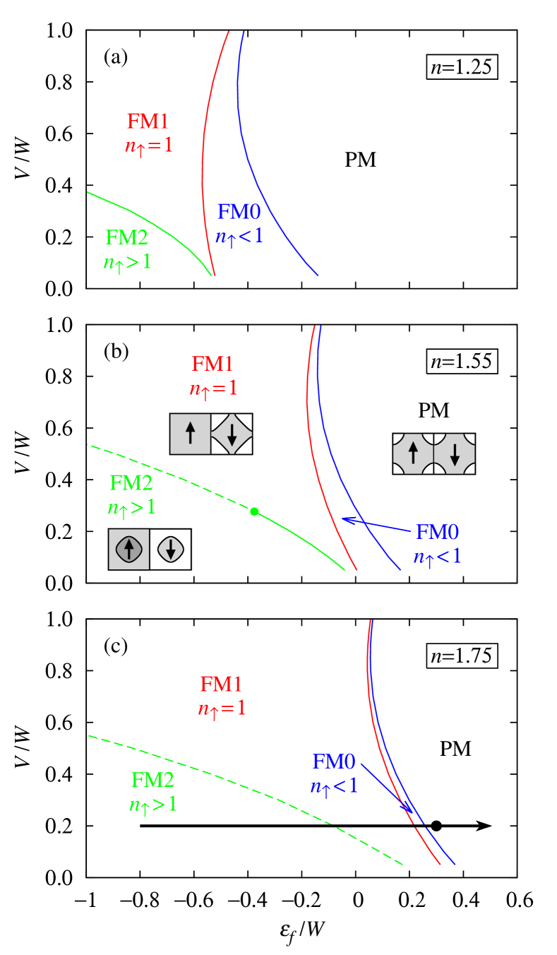
Figure 2: (Color online) Phase diagrams (a) for $n=1.25$, (b) for $n=1.55$, and (c) for $n=1.75$. The solid lines indicate second-order phase transitions and the dashed lines indicate first-order phase transitions. The circle in (b) represents the end point of the first-order phase transition. In (b), we also show the Fermi-surface structures in these phases schematically. The lower hybridized band is occupied by electrons in the lightly shaded area. In the darkly shaded area, both the lower and upper hybridized bands are filled by electrons. The bold arrow in (c) indicates the parameters for which physical quantities shown in Figs. 3 and 4 are calculated. The circle in (c) indicates the parameter set for which the magnetic field dependences of the physical quantities are calculated (Figs. 5 and 6).

All the three ferromagnetic phases discussed above, FM0, FM1, and FM2, appear. For $n=1.25$, Fig. 2(a), all the phase transition are of second order. On the other hand, the FM1-FM2 transition is of first order for $n=1.75$ [Fig. 2(c)]. Here, we discuss the reason why the order of the FM1-FM2 transition changes with $n$. As we will show later [Fig. 3(a)], the polarization of the conduction electrons $M_{c}=n_{c\uparrow}-n_{c\downarrow}=(n_{\uparrow}-n_{f\uparrow})-(n_{\downarrow}-n_{f\downarrow})$ is small even in the ferromagnetic phases. Thus, the magnetization in FM1 ($n_{\uparrow}=1$) is approximated as $M=n_{f\uparrow}-n_{f\downarrow}\simeq n_{\uparrow}-n_{\downarrow}=2n_{\uparrow}-n=2-n$, and $M$ is smaller for larger $n$. In FM2, $M$ is almost 1, irrespective of $n$. Then, the change in $M$ at the FM1-FM2 transition is larger for large $n$. Such a large change in the electronic state may not occur continuously but tends to occur through a first order transition, as for $n=1.75$. A similar discussion has been applied for the valence transition in the periodic Anderson model with an interorbital Coulomb interaction. Kubo (2011a) For an intermediate value of $n$, we find the end point of the first order transition as shown in Fig. 2(b). On the second order transition line, the magnetic susceptibility diverges. At the end point, the valence susceptibility $dn_{f}/d\epsilon_{f}$ also diverges. Such fluctuations of various kinds may induce interesting phenomena, e.g., unconventional superconductivity.

From these phase diagrams, we gain an insight into the effects of pressure on Ce and Yb compounds. $\epsilon_{f}$ describes the one-electron level for a Ce compound and one-hole level for an Yb compound. Then, $\epsilon_{f}$ will increase by pressure for a Ce compound, but will decrease for an Yb compound, since negatively charged ions surrounding a positively charged rare-earth ion will become close to the rare-earth ion. On the other hand, $V$ and $W$ increase under a pressure irrespective of compounds. Thus, it is not obvious whether the effect of pressure is opposite or not between Ce and Yb compounds. In the present model, there are two independent parameters $\epsilon_{f}/W$ and $V/W$ except for the overall energy scale. From the above phase diagrams, we observe that we can change the electronic state easier by varying $\epsilon_{f}/W$, e.g., along the bold arrow in Fig. 2(c), than by varying $V/W$, and we may ignore the change in $V/W$ under pressure as an approximation.

Here, we further assume that the changes by a pressure $p$ are approximated linear in $p$. Then, we can express $\epsilon_{f}=\epsilon^{(0)}_{f}+a_{\epsilon_{f}}p$ and $W=W^{(0)}+a_{W}p$, where $\epsilon^{(0)}_{f}$ is the $f$ level at $p=0$, $W^{(0)}$ is the band width at $p=0$, $a_{\epsilon_{f}}>0$ for Ce compounds, $a_{\epsilon_{f}}<0$ for Yb compounds, and $a_{W}>0$. The ratio $\epsilon_{f}/W$ under pressure is given by

$$\frac{\epsilon_{f}}{W}=\frac{\epsilon^{(0)}_{f}+\tilde{a}_{\epsilon_{f}}p}{W^{(0)}},$$ (23)

with $\tilde{a}_{\epsilon_{f}}=a_{\epsilon_{f}}-a_{W}\epsilon^{(0)}_{f}/W^{(0)}$. For Ce compounds with $\epsilon^{(0)}_{f}<0$, typical for magnetically ordered materials at ambient pressure, we obtain $\tilde{a}_{\epsilon_{f}}>0$. For Yb compounds with $\epsilon^{(0)}_{f}>0$, typical for paramagnetic materials at ambient pressure, $\tilde{a}_{\epsilon_{f}}<0$. Thus, magnetically ordered states of Ce compounds will be destabilized by pressure, and paramagnetic Yb compounds may become magnetic under pressure. In the above sense, the pressure effects on Ce and Yb compounds are opposite.

However, the pressure effects on Ce compounds with $\epsilon^{(0)}_{f}>0$ and on Yb compounds with $\epsilon^{(0)}_{f}<0$ depend on the details of the parameters. Thus, in principle, paramagnetic Ce compounds can become magnetic and magnetically ordered states of Yb compounds can become paramagnetic under pressure, when the effect of pressure on the band width is large.

IV.2 $\epsilon_{f}$ dependence

Next, we show $\epsilon_{f}$ dependences of physical quantities. In Fig. 3, we show the magnetization, the kinetic energy $\epsilon_{k_{\text{F}\sigma}}$ of the conduction electron at the Fermi momentum, and the effective mass for $n=1.75$ and $V/W=0.2$.

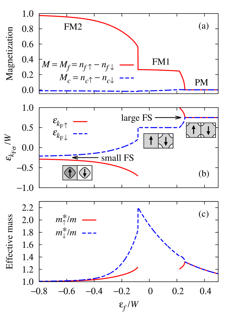
Figure 3: (Color online) Physical quantities as functions of $\epsilon_{f}$ for $n=1.75$ and $V/W=0.2$. (a) magnetization $M=M_{f}$ and polarization of the conduction band $M_{c}$, (b) kinetic energy $\epsilon_{k_{\text{F}\sigma}}$ of the conduction electron at the Fermi momentum, and (c) effective mass $m^{*}_{\sigma}$. In (b), we show the Fermi-surface (FS) structure in each phase schematically.

$\epsilon_{f}$ is varied along the bold arrow in Fig. 2(c).

The magnetization [Fig. 3(a)] is almost 1 in FM2, decreases by increasing $\epsilon_{f}$, and the state changes to the FM1, FM0, and PM states. Even in the ferromagnetic phases, the polarization of the conduction electrons $M_{c}$ is small, since the loss of the kinetic energy is large for a large polarization of the conduction electrons.

In Fig. 3(b), we show $\epsilon_{k_{\text{F}\sigma}}$. In the present theory, physical quantities depend on momentum $\mathbf{k}$ only through $\epsilon_{\mathbf{k}}$, and here we show $\epsilon_{k_{\text{F}\sigma}}$ instead of the Fermi momentum $k_{\text{F}\sigma}$ itself. If the explicit form of the dispersion $\epsilon_{\mathbf{k}}$ is given, we can extract $k_{\text{F}\sigma}$ from $\epsilon_{k_{\text{F}\sigma}}$. In FM2, $\epsilon_{k_{\text{F}\sigma}}$ has a value around that for the small Fermi-surface state. In FM1, the Fermi surface for the up-spin state disappears. In PM, the large Fermi-surface state realizes.

Figure 3(c) shows the effective mass. For the periodic Anderson model, the effective mass is usually defined by the inverse of the renormalization factor for the $f$ electrons. This is reasonable as long as the Fermi surface is composed mainly of $f$ electrons as in a state with very large effective-mass. However, in magnetically ordered states and in a state under a magnetic field, the $f$-electron contribution to the Fermi surface can become small. Thus, we should better to define the effective mass by the renormalization of the hybridized band. In this study, we define the spin-dependent effective-mass $m^{*}_{\sigma}$ by the jump in the momentum distribution at the Fermi momentum:

$$\frac{m^{*}_{\sigma}}{m}=\frac{1}{\Delta n_{c\sigma}(k_{\text{F}\sigma})+\Delta n_{f\sigma}(k_{\text{F}\sigma})},$$ (24)

where $m$ is the bare electron mass.

The effective mass in FM2 becomes small by decreasing $\epsilon_{f}$, since the magnetization becomes large and the correlation effects become weaker. In the PM phase, the number of $f$ electrons decreases as $\epsilon_{f}$ increases, and then, the correlation effects becomes less significant and the effective mass decreases. In between, in FM1, the effective mass for the down-spin electrons has a peak. Note that we cannot define the effective mass for the up-spin state in FM1, since there is no Fermi surface for the up-spin states.

Figure 4(a) shows the number of electrons $n_{\sigma}$ with spin $\sigma$ and the number of $f$ electrons $n_{f\sigma}$ with spin $\sigma$.

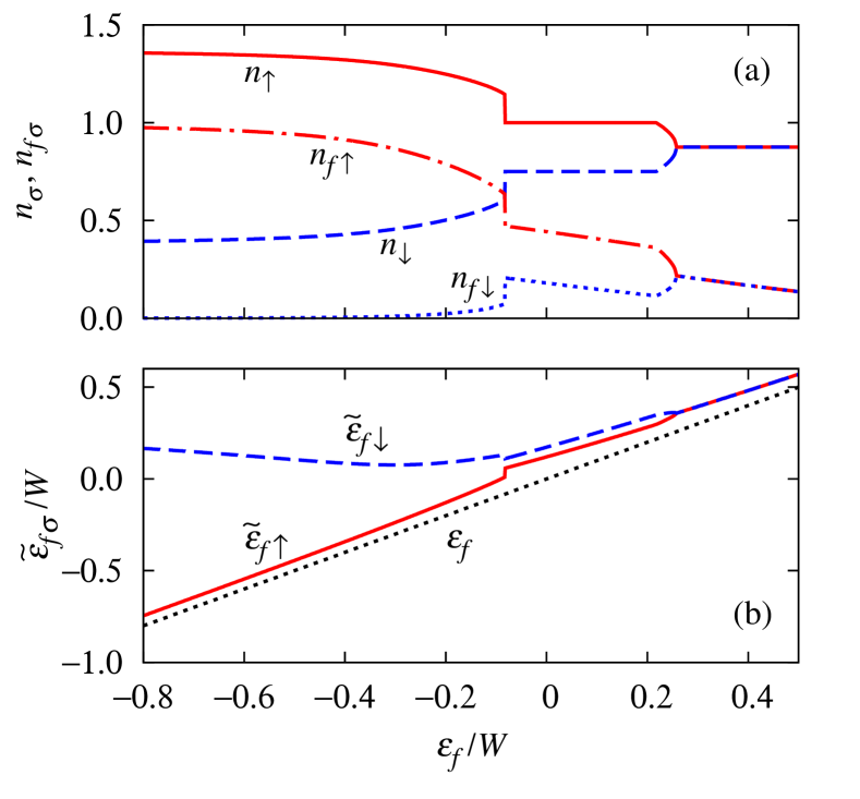
Figure 4: (Color online) Physical quantities as functions of $\epsilon_{f}$ for $n=1.75$ and $V/W=0.2$. (a) $n_{\sigma}$ and $n_{f\sigma}$ and (b) $\tilde{\epsilon}_{f\sigma}$. The dotted line in (b) indicates the bare $f$-level $\epsilon_{f}$.

In FM2, the polarization of $f$ electrons is almost complete, that is, $n_{f\uparrow}\simeq 1$ and $n_{f\downarrow}\simeq 0$. In FM1, i.e., the half-metallic state, $n_{\uparrow}=1$.

Figure 4(b) shows the renormalized $f$-level. In FM2, $\tilde{\epsilon}_{f\downarrow}$ is much larger than $\epsilon_{k^{\text{(S)}}_{\text{F}}}=-0.25W$ and $\tilde{\epsilon}_{f\uparrow}\simeq\epsilon_{f}$. In FM1, FM0, and PM, $\epsilon_{f}$ is larger than $\epsilon_{k^{\text{(S)}}_{\text{F}}}$, and the renormalization effect is weak, that is, $\tilde{\epsilon}_{f\sigma}\simeq\epsilon_{f}$.

The overall behaviours of the magnetization [Fig. 3(a)] and the effective mass [Fig. 3(c)] as functions of $\epsilon_{f}$ are similar to those as functions of pressure in UGe₂. Oomi et al. (1998); Saxena et al. (2000); Tateiwa et al. (2001); Settai et al. (2002); Pfleiderer and Huxley (2002) However, further efforts are necessary to understand the experimental results based on the present theory. For example, we should calculate the electrical resistivity to discuss directly the effective mass deduced from $A$ coefficient, since we cannot resolve the spin components of the effective mass from $A$.

IV.3 Magnetic field effect

Now, we discuss the magnetic field effect. We choose $n=1.75$, $V/W=0.2$, and $\epsilon_{f}/W=0.3$, which are indicated by the circle in Fig. 2(c). For this parameter set, the system is paramagnetic without a magnetic field, but near the ferromagnetic phase boundary. The effective mass is not large for this parameter set [see Fig. 3(c)]. If we assume a paramagnetic state with a much deeper $f$-level, we can obtain a large effective mass, but such a paramagnetic state is unstable against magnetic order due to the large Coulomb interaction $U$. Thus, we have chosen the above parameter set. We believe that the qualitative aspects of $f$-electron systems under a magnetic field are still captured by the present simple model with $U\rightarrow\infty$.

Figure 5 shows the $H$ dependences of the magnetization, the kinetic energy $\epsilon_{k_{\text{F}\sigma}}$ of the conduction electron at the Fermi momentum, and the effective mass.

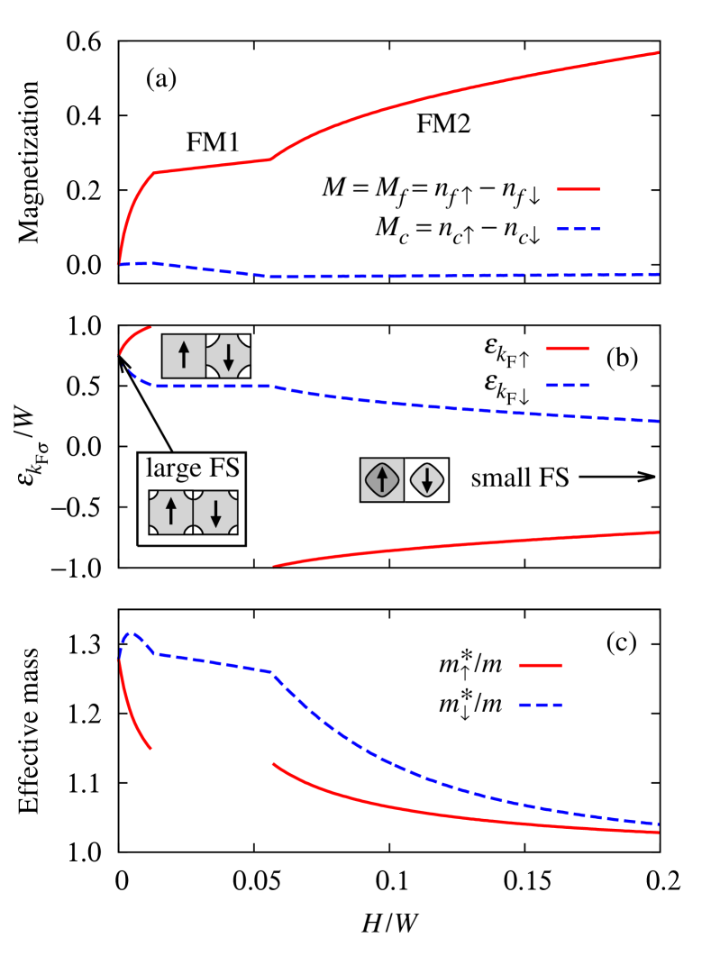
Figure 5: (Color online) Physical quantities as functions of $H$ for $n=1.75$, $V/W=0.2$, and $\epsilon_{f}/W=0.3$. (a) magnetization $M=M_{f}$ and polarization of the conduction band $M_{c}$, (b) kinetic energy $\epsilon_{k_{\text{F}\sigma}}$ of the conduction electron at the Fermi momentum, and (c) effective mass $m^{*}_{\sigma}$. In (b), we show the Fermi-surface structure in each phase schematically.

The polarization of the conduction band $M_{c}$ is always small as in the ferromagnetic phases without magnetic field. The magnetization $M=M_{f}$ increases continuously as a function of $H$. The magnetization curve is similar to that in YbRh₂Si₂, Tokiwa et al. (2005) if we regard the anomaly around 10 T in YbRh₂Si₂ at ambient pressure as the transition to FM1. The Fermi-surface structure changes continuously from the large Fermi-surface in PM to the small Fermi-surface in FM2. The effective mass decreases by a magnetic field except for a small-$H$ region, since a magnetic field polarizes the $f$ electrons and the correlation effect becomes weak. In the small-$H$ region, $n_{f\uparrow}$ increases by $H$ but $n_{f\downarrow}$ is not very small [see Fig. 6(a)], and the effect of the Coulomb interaction becomes stronger for the down-spin state. Then, the effective mass for the down-spin electrons increases as $H$ in the small-$H$ region, and has a peak.

Figure 6 shows the magnetic field dependences of $n_{\sigma}$, $n_{f\sigma}$, and $\tilde{\epsilon}_{f\sigma}$.

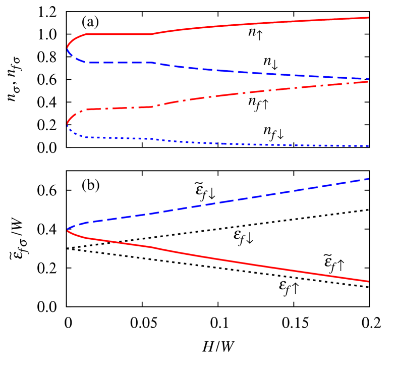
Figure 6: (Color online) Physical quantities as functions of $H$ for $n=1.75$, $V/W=0.2$, and $\epsilon_{f}/W=0.3$. (a) $n_{\sigma}$ and $n_{f\sigma}$ and (b) $\tilde{\epsilon}_{f\sigma}$. The dotted lines in (b) indicate the bare $f$-levels $\epsilon_{f\sigma}=\epsilon_{f}-\sigma H$.

By increasing $H$, the system turns into FM1 with $n_{\uparrow}=1$. By increasing $H$ further, the system turns into FM2, and the polarization of $f$ electrons approaches the saturation value asymptotically, i.e., $n_{f\uparrow}\rightarrow 1$ and $n_{f\downarrow}\rightarrow 0$. The renormalized $f$-level changes monotonically. $\tilde{\epsilon}_{f\uparrow}$ becomes very close to $\epsilon_{f\uparrow}$ by increasing $H$, since the correlation effects on the up-spin electrons are weak for $n_{f\downarrow}\rightarrow 0$.

There are kinks in all the above quantities at the transition points to FM1 and from FM1 to FM2. The kinks in $\tilde{\epsilon}_{f\sigma}$ [Fig. 6(b)] are weak and invisible on this scale. While these ferromagnetic transitions are continuous, they are not crossovers even under magnetic fields. We discuss this issue in the next subsection.

IV.4 Order of the ferromagnetic phase transitions

In this subsection, we discuss the order of the phase transitions. It is usual that between ferromagnetic states, the transition is a first-order phase transition or just a crossover, not a phase transition, since the symmetry is the same between the ferromagnetic states. However, in the present model, the transitions between the ferromagnetic phases, FM0, FM1, and FM2, can be phase transitions even if they are continuous. To explicitly demonstrate it, we show the energy $e$ per site in Fig. 7 as a function of $\epsilon_{f}$ for $n=1.75$ and $V/W=0.2$ without a magnetic field, around the phase transition points.

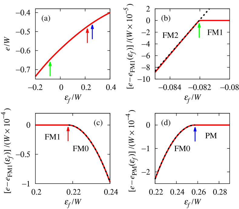
Figure 7: (Color online) Energy $e$ per site as a function of $\epsilon_{f}$ for $n=1.75$ and $V/W=0.2$. (a) energy in a wide range of $\epsilon_{f}$. Arrows indicate the phase transition points. (b)-(d) show energy around each phase transition point: (b) between FM2 and FM1, (c) between FM1 and FM0, and (d) between FM0 and PM. Energy in phase X is fitted by a polynomial function $e_{\text{X}}(\epsilon_{f})$ and we subtracted $e_{\text{X}}(\epsilon_{f})$ from $e$ in (b)-(d). This difference is linear in $\epsilon_{f}$ in (b) and is quadratic in $\epsilon_{f}$ in (c) and (d) as indicated by the dotted lines.

The first derivative of $e$ has a jump at the FM2-FM1 boundary as shown in Fig. 7(b), and it is a first-order phase transition. The second derivative of $e$ has a jump at the FM1-FM0 boundary as shown in Figs. 7 (c), and it is a second-order phase transition, not a crossover. The FM0-PM phase transition is also of second order.

We can show that when the magnetization $M$ changes its slope but is continuous at a point, as in Figs. 3(a) and 5(a), it is a second-order phase transition point (see Appendix). That is, to cause a second-order phase transition, it is not necessary to break symmetry. Behind such a second-order phase transition between ferromagnetic states in the present model, the topology of the Fermi surface changes, i.e., it is a Lifshitz transition. Note that while the originally proposed Lifshitz transition is of 2.5 order, Lifshitz (1960) the present Lifshitz transition accompanying magnetism is of second order.

Note also that the transitions to FM1 and from FM1 to FM2 under magnetic fields shown in Figs. 5 and 6 are second-order phase transitions, while, in ordinary cases, a continuous ferromagnetic transition becomes a crossover under a finite magnetic field. These transitions under magnetic fields are possible even for $U=0$.

At finite temperatures, the second-order phase transitions between ferromagnetic phases would become crossovers, since the Fermi surface is not well defined at finite temperatures. On the other hand, first-order phase transitions are possible even at finite temperatures.

V Antiferromagnetic states

In the present study, we have assumed uniform states: paramagnetic and ferromagnetic. The calculated results have been interpreted with the aid of the schematic bands shown in Fig. 1. A similar discussion may be applicable to antiferromagnetic states.

We show the schematic bands expected in antiferromagnetic states with a two-sublattice structure in Fig. 8.

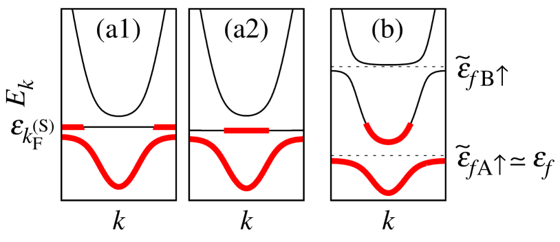
Figure 8: (Color online) Schematic band structures expected in antiferromagnetic phases. In a weakly polarized state, the band structure like (a1) or (a2) will realize. In a strongly polarized state, the band structure shown in (b) will realize. $E_{k}$ denotes the quasi-particle energy. The bold lines indicate the states occupied by electrons.

In a weak antiferromagnetic state, the difference of the renormalized $f$-level between A and B sublattices is small, and we may obtain the band structure by simply folding the Brillouin zone as shown in Fig. 8(a1). In a strongly polarized antiferromagnetic state, the renormalized $f$-levels will be much different between A and B sublattices. We show a schematic band structure in such a state in Fig. 8(b), by assuming that the $f$ orbitals on the A sublattice are mainly occupied by up-spin electrons and the $f$ orbitals on the B sublattice are mainly occupied by down-spin electrons. The effective $f$-level $\tilde{\epsilon}_{f\text{A}\uparrow}$ for up spin on the A sublattice is almost the same as the bare $f$-level $\epsilon_{f}$ and the effective $f$-level $\tilde{\epsilon}_{f\text{B}\uparrow}$ for up spin on the B sublattice is much higher than the Fermi level [cf. the ferromagnetic case Fig. 1(d)]. Note that $\tilde{\epsilon}_{f\text{A}\uparrow}=\tilde{\epsilon}_{f\text{B}\downarrow}$ and $\tilde{\epsilon}_{f\text{B}\uparrow}=\tilde{\epsilon}_{f\text{A}\downarrow}$. In the strongly polarized state, the electronic state around the Fermi surface is mainly composed of the conduction-electron states.

Since the topology of the Fermi surfaces are different between (a1) and (b), a phase transition takes place as the antiferromagnetic moment develops provided the system first turns into the antiferromagnetic state with the band structure (a1) from the paramagnetic state. Indeed, such a phase transition in the antiferromagnetic phase has been found in the Kondo lattice model Watanabe and Ogata (2007); Lanatà et al. (2008); Martin et al. (2010) and in the periodic Anderson model, Watanabe and Ogata (2009) and possibility to explain the Fermi-surface reconstruction in CeRh_1-xCo_xIn₅ Goh et al. (2008) and in YbRh₂Si₂ with chemical pressure Friedemann et al. (2009) has been discussed.

In addition, the direct transition from the paramagnetic state to the antiferromagnetic state with the band structure shown in Fig. 8(a2), which has the same topology of the Fermi surface as in (b), is possible, since the band originates from the $f$ orbital is very flat. Note that the band structure (a2) is not obtained by simply folding that in the paramagnetic state, and the effects of the change in the Fermi surface would be drastic. This transition has also been found in the Kondo lattice model Watanabe and Ogata (2007); Lanatà et al. (2008) and in the periodic Anderson model, Watanabe and Ogata (2009) and has been proposed as a possible mechanism to explain the change in the Hall coefficient of YbRh₂Si₂ at the antiferromagnetic quantum critical point. Paschen et al. (2004) Note that we expect a mass enhancement around such a magnetic transition point as we have shown for the ferromagnetic case. Thus, this transition may also be a candidate for the mechanism of the Fermi-surface change and the enhancement of the effective mass around the antiferromagnetic transition point observed by the de Haas-van Alphen experiments under pressure on CeRh₂Si₂, Araki et al. (2001) CeRhIn₅, Shishido et al. (2005) and CeIn₃. Settai et al. (2005)

VI Summary

We have studied the ferromagnetism and the magnetic field effect in the periodic Anderson model by using the Gutzwiller theory. There are three ferromagnetic phases, FM0, FM1, and FM2. The Fermi-surface structure changes according to the magnetic state. The PM state has a large Fermi-surface, the FM0 state is a weak ferromagnetic state, the FM1 state is a half-metallic state without a Fermi surface for up-spin electrons, and the FM2 state has a small Fermi-surface. The effective mass has a peak in the FM1 phase as a function of $\epsilon_{f}$.

The transitions between these ferromagnetic phases can be second-order phase transitions, while we cannot define the order parameter in an ordinary way due to the absence of symmetry breaking. These second-order phase transitions originate from the change in the Fermi-surface topology and are called Lifshitz transitions. We have found that the present Lifshitz transitions accompanying magnetism are of second order, while the originally proposed Lifshitz transition is of 2.5 order. Lifshitz (1960)

According to the theory of phase transitions, if the symmetry is broken spontaneously, a phase transition takes place. However, the converse is not necessarily true. For example, the liquid-vapor transition of water is a first-order phase transition without symmetry breaking. In the present paper, we have shown that a second-order transition is also possible without symmetry breaking.

In the present model with $U\rightarrow\infty$, a paramagnetic state with a large mass enhancement is not attained, since the magnetically ordered state becomes stable against the paramagnetic state before the effective mass becomes very large. Thus, we should revise the present model to describe the heavy-fermion state quantitatively, e.g., by using a finite value of $U$ and/or by introducing the orbital degrees of freedom of $f$ electrons. Rice and Ueda (1986) It is an important future problem.

*

Appendix A Sufficient condition for a second-order phase transition

A second-order phase transition is defined by a jump in the second derivative of the free energy (or energy at zero temperature). We consider the system described by the free energy $F(x,M)$. $x$ is a controlling parameter such as magnetic field, pressure, $f$-electron level, and temperature. $M$ represents a physical quantity such as magnetization and $f$-electron number. The physical quantity $M(x)$ at $x$ is determined by minimizing $F(x,M)$ with respect to $M$:

$$\left.\frac{\partial F(x,M)}{\partial M}\right|_{M=M(x)}=0.$$ (25)

Then, the first derivative of the free energy $F(x,M(x))$ at $x$ is

$$\frac{dF(x,M(x))}{dx}=\left.\frac{\partial F(x,M)}{\partial x}\right|_{M=M(x)}.$$ (26)

If $M(x)$ changes discontinuously at a point, the first derivative has a jump at this point and it is a first-order phase transition. The second derivative is given by

$$\begin{split}\frac{d^{2}F(x,M(x))}{dx^{2}}=&\left.\frac{\partial^{2}F(x,M)}{\partial x^{2}}\right|_{M=M(x)}\\ +&\left.\frac{\partial^{2}F(x,M)}{\partial x\partial M}\right|_{M=M(x)}\frac{dM(x)}{dx}.\end{split}$$ (27)

Then, if $M(x)$ is continuous and $dM(x)/dx$ is discontinuous at a point, it is a second-order phase transition.

We have not assumed that $M(x)=0$ below or above the transition point. Thus, the above discussion does not require that $M$ is an order parameter to describe symmetry breaking.

References

- Besnus et al. (1985) M. J. Besnus, J. P. Kappler, P. Lehmann, and A. Meyer, Solid State Commun. 55, 779 (1985).
- Haen et al. (1987) P. Haen, J. Flouquet, F. Lapierre, P. Lejay, and G. Remenyi, J. Low Temp. Phys. 67, 391 (1987).
- van der Meulen et al. (1991) H. P. van der Meulen, A. de Visser, J. J. M. Franse, T. T. J. M. Berendschot, J. A. A. J. Perenboom, H. van Kempen, A. Lacerda, P. Lejay, and J. Flouquet, Phys. Rev. B 44, 814 (1991).
- Aoki et al. (1993) H. Aoki, S. Uji, A. K. Albessard, and Y. Ōnuki, Phys. Rev. Lett. 71, 2110 (1993).
- Tokiwa et al. (2005) Y. Tokiwa, P. Gegenwart, T. Radu, J. Ferstl, G. Sparn, C. Geibel, and F. Steglich, Phys. Rev. Lett. 94, 226402 (2005).
- Rourke et al. (2008) P. M. C. Rourke, A. McCollam, G. Lapertot, G. Knebel, J. Flouquet, and S. R. Julian, Phys. Rev. Lett. 101, 237205 (2008).
- (7) H. Pfau, R. Daou, S. Lausberg, H. R. Naren, M. Brando, S. Friedemann, S. Wirth, T. Westerkamp, U. Stockert, P. Gegenwart, C. Krellner, C. Geibel, G. Zwicknagl, and F. Steglich, arXiv:1302.6867 .
- Pourret et al. (2013) A. Pourret, G. Knebel, T. D. Matsuda, G. Lapertot, and J. Flouquet, J. Phys. Soc. Jpn. 82, 053704 (2013).
- Pfleiderer and Huxley (2002) C. Pfleiderer and A. D. Huxley, Phys. Rev. Lett. 89, 147005 (2002).
- Saxena et al. (2000) S. S. Saxena, P. Agarwal, K. Ahilan, F. M. Grosche, R. K. W. Haselwimmer, M. J. Steiner, E. Pugh, I. R. Walker, S. R. Julian, P. Monthoux, G. G. Lonzarich, A. Huxley, I. Sheikin, D. Braithwaite, and J. Flouquet, Nature 406, 587 (2000).
- Tateiwa et al. (2001) N. Tateiwa, T. C. Kobayashi, K. Hanazono, K. Amaya, Y. Haga, R. Settai, and Y. Ōnuki, J. Phys.: Condens. Matter 13, L17 (2001).
- Oomi et al. (1998) G. Oomi, T. Kagayama, and Y. Ōnuki, J. Alloys Compd. 271-273, 482 (1998).
- Settai et al. (2002) R. Settai, M. Nakashima, S. Araki, Y. Haga, T. C. Kobayashi, N. Tateiwa, H. Yamagami, and Y. Ōnuki, J. Phys.: Condens. Matter 14, L29 (2002).
- Terashima et al. (2001) T. Terashima, T. Matsumoto, C. Terakura, S. Uji, N. Kimura, M. Endo, T. Komatsubara, and H. Aoki, Phys. Rev. Lett. 87, 166401 (2001).
- Terashima et al. (2002) T. Terashima, T. Matsumoto, C. Terakura, S. Uji, N. Kimura, M. Endo, T. Komatsubara, H. Aoki, and K. Maezawa, Phys. Rev. B 65, 174501 (2002).
- Haga et al. (2002) Y. Haga, M. Nakashima, R. Settai, S. Ikeda, T. Okubo, S. Araki, T. C. Kobayashi, N. Tateiwa, and Y. Ōnuki, J. Phys.: Condens. Matter 14, L125 (2002).
- Settai et al. (2003) R. Settai, M. Nakashima, H. Shishido, Y. Haga, H. Yamagami, and Y. Ōnuki, Acta Phys. Pol. B 34, 725 (2003).
- Rice and Ueda (1986) T. M. Rice and K. Ueda, Phys. Rev. B 34, 6420 (1986).
- Fazekas and Brandow (1987) P. Fazekas and B. H. Brandow, Phys. Scr. 36, 809 (1987).
- Reynolds et al. (1992) A. M. Reynolds, D. M. Edwards, and A. C. Hewson, J. Phys.: Condens. Matter 4, 7589 (1992).
- Dorin and Schlottmann (1993a) V. Dorin and P. Schlottmann, J. Appl. Phys. 73, 5400 (1993a).
- Dorin and Schlottmann (1993b) V. Dorin and P. Schlottmann, Phys. Rev. B 47, 5095 (1993b).
- Kubo (2013) K. Kubo, Phys. Status Solidi C 10, 544 (2013).
- Kubo (2011a) K. Kubo, J. Phys. Soc. Jpn. 80, 063706 (2011a).
- Kubo (2011b) K. Kubo, J. Phys. Soc. Jpn. 80, 114711 (2011b).
- Yu. Irkhin and Katsnelson (1991) V. Yu. Irkhin and M. I. Katsnelson, Z. Phys. B 82, 77 (1991).
- Watanabe (2000) S. Watanabe, J. Phys. Soc. Jpn. 69, 2947 (2000).
- Viola Kusminskiy et al. (2008) S. Viola Kusminskiy, K. S. D. Beach, A. H. Castro Neto, and D. K. Campbell, Phys. Rev. B 77, 094419 (2008).
- Beach and Assaad (2008) K. S. D. Beach and F. F. Assaad, Phys. Rev. B 77, 205123 (2008).
- Peters et al. (2012) R. Peters, N. Kawakami, and T. Pruschke, Phys. Rev. Lett. 108, 086402 (2012).
- Bercx and Assaad (2012) M. Bercx and F. F. Assaad, Phys. Rev. B 86, 075108 (2012).
- Peters and Kawakami (2012) R. Peters and N. Kawakami, Phys. Rev. B 86, 165107 (2012).
- Miyake and Ikeda (2006) K. Miyake and H. Ikeda, J. Phys. Soc. Jpn. 75, 033704 (2006).
- Suzuki and Harima (2010) M.-T. Suzuki and H. Harima, J. Phys. Soc. Jpn. 79, 024705 (2010).
- Lifshitz (1960) I. M. Lifshitz, Sov. Phys. JETP 11, 1130 (1960).
- Watanabe and Ogata (2007) H. Watanabe and M. Ogata, Phys. Rev. Lett. 99, 136401 (2007).
- Lanatà et al. (2008) N. Lanatà, P. Barone, and M. Fabrizio, Phys. Rev. B 78, 155127 (2008).
- Martin et al. (2010) L. C. Martin, M. Bercx, and F. F. Assaad, Phys. Rev. B 82, 245105 (2010).
- Watanabe and Ogata (2009) H. Watanabe and M. Ogata, J. Phys. Soc. Jpn. 78, 024715 (2009).
- Goh et al. (2008) S. K. Goh, J. Paglione, M. Sutherland, E. C. T. O’Farrell, C. Bergemann, T. A. Sayles, and M. B. Maple, Phys. Rev. Lett. 101, 056402 (2008).
- Friedemann et al. (2009) S. Friedemann, T. Westerkamp, M. Brando, N. Oeschler, S. Wirth, P. Gegenwart, C. Krellner, C. Geibel, and F. Steglich, Nat. Phys. 5, 465 (2009).
- Paschen et al. (2004) S. Paschen, T. Lühmann, S. Wirth, P. Gegenwart, O. Trovarelli, C. Geibel, F. Steglich, P. Coleman, and Q. Si, Nature 432, 881 (2004).
- Araki et al. (2001) S. Araki, R. Settai, T. C. Kobayashi, H. Harima, and Y. Ōnuki, Phys. Rev. B 64, 224417 (2001).
- Shishido et al. (2005) H. Shishido, R. Settai, H. Harima, and Y. Ōnuki, J. Phys. Soc. Jpn. 74, 1103 (2005).
- Settai et al. (2005) R. Settai, T. Kubo, T. Shiromoto, D. Honda, H. Shishido, K. Sugiyama, Y. Haga, T. D. Matsuda, K. Betsuyaku, H. Harima, T. C. Kobayashi, and Y. Ōnuki, J. Phys. Soc. Jpn. 74, 3016 (2005).