Automated Calibration System for a High-Precision Measurement of Neutrino Mixing Angle $\theta_{13}$ with the Daya Bay Antineutrino Detectors

Abstract

We describe the automated calibration system for the antineutrino detectors in the Daya Bay Neutrino Experiment. This system consists of 24 identical units instrumented on 8 identical 20-ton liquid scintillator detectors. Each unit is a fully automated robotic system capable of deploying an LED and various radioactive sources into the detector along given vertical axes. Selected results from performance studies of the calibration system are reported.

1 Introduction

Transformations among three active neutrino flavors, also known as neutrino oscillations, have been firmly established by solar, atmospheric, long-baseline accelerator, and long-baseline reactor neutrino experiments [1, 2]. Under the three-neutrino framework, mixing among neutrinos can be described by the so-called PMNS matrix [3, 4], a 3x3 unitary matrix which conventionally gets parametrized by three independent “Euler angles” $\theta_{12}$ (solar mixing angle), $\theta_{23}$ (atmospheric mixing angle), and $\theta_{13}$, one complex CP phase $\delta$, and two complex Majorana phases if neutrinos are Majorana particles. $\theta_{23}$ ($\sim$45 deg) and $\theta_{12}$ ($\sim$ 30 deg) have been measured to 5% accuracy [1]. However, $\theta_{13}$ had remained elusive until a series of recent measurements worldwide [9, 5, 6, 7, 8], particularly after a definitive measurement of electron-antineutrino disappearance at the Daya Bay reactors [9].

The Daya Bay Reactor Neutrino Experiment is located on the Daya Bay reactor power plant campus in southern China. The power plant currently hosts six 2.9 GW_th pressurized water reactors: the Daya Bay complex has two reactors and the Ling Ao complex has the other four. The layout of the Daya Bay experiment is shown in Fig. 1. The experiment has 8 “identical” antineutrino detectors (AD) deployed in the three underground experimental halls: two near halls to monitor the reactor antineutrino fluxes from the Daya Bay and the Ling Ao complexes and one far hall to measure combined flux around a baseline where maximal oscillation occurs. The near-far arrangement of the ADs can effectively cancel correlated uncertainties in reactor antineutrino flux and detector efficiency, leading to high sensitivity to $\sin^{2}2\theta_{13}$ [10].

A fully automated calibration system was designed and constructed to calibrate AD responses and to monitor their stability regularly. The rest of this article is organized as follows. In Sec. 2 of the paper, we briefly describe the Daya Bay reactor neutrino experiment and design requirements of the calibration system. Design details will be given in Sec. 3, followed by a discussion of operational tests, quality control, and internal calibration of the system in Sec. 4. We will discuss calibration data taken during the commissioning tests, as well as in-situ calibration results during the physics running in Sec. 5, followed by a summary in Sec 6.

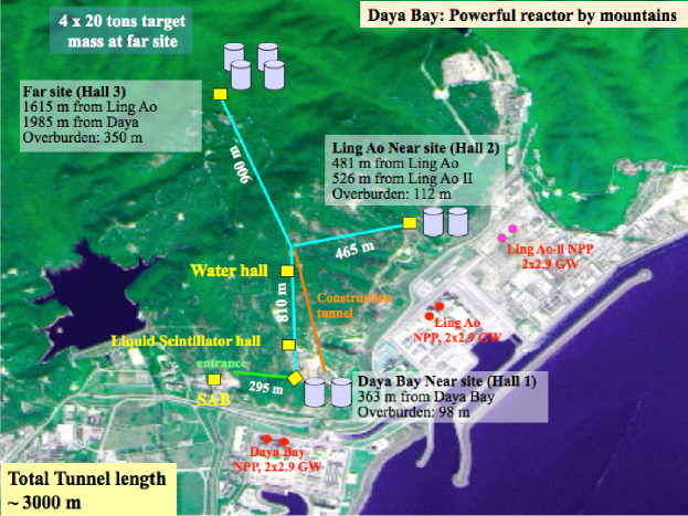
Figure 1: The layout of the Daya Bay experiment.

2 Requirements of the calibration system

2.1 Overview of experiment

The primary goal of the Daya Bay reactor neutrino experiment is to make a sensitive measurement of $\sin^{2}2\theta_{13}$ to a precision <0.01 (90% confidence level). Like other reactor neutrino experiments, electron-type antineutrinos are detected via the inverse beta decay (IBD) process:

$$\bar{\nu_{e}}+p\rightarrow e^{+}+n\,.$$ (1)

In this reaction, neutrino energy $E_{\nu}$ can be reconstructed by the kinetic energy of the positron $T_{e^{+}}$ as

$$E_{\nu}\simeq T_{e^{+}}+1.8\rm{MeV}\,.$$ (2)

Detailed discussion of the Daya Bay anti-neutrino detectors (AD) can be found elsewhere [10, 11]. For context, we reiterate a few key features here. Fig. 2 shows the design of the AD.

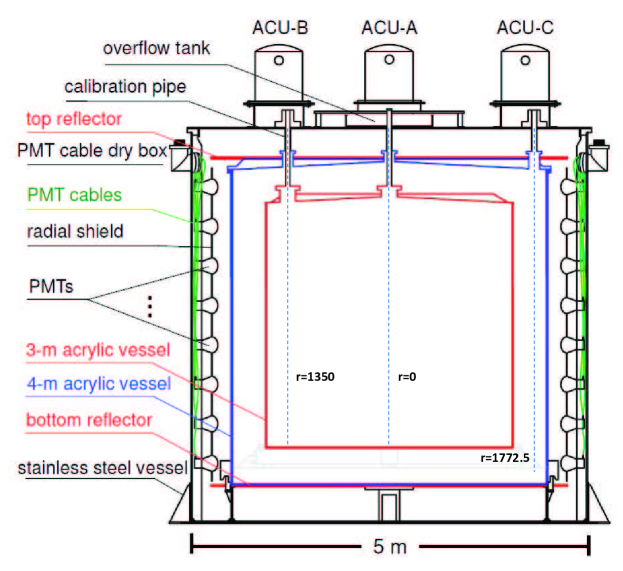
Figure 2: An illustration of the Daya Bay antineutrino detector structure. The inner acrylic vessel (IAV) holds the target, Gd-doped liquid scintillator. The outer acrylic vessel (OAV) holds undoped liquid scintillator as the gamma catcher. The outermost zone inside the stainless steel tank where PMTs are located is filled with mineral oil. See text for more details. The target zone is monitored by two ACUs, A (r=0 cm) and B (r=135.0 cm). ACU C (r=177.25 cm) monitors the gamma catcher zone. Three vertical source deployment axes are indicated by the dashed lines in the figure.

The detector has three zones; the innermost acrylic vessel (IAV) with 3-meter diameter holds the target - 20t Gd doped LAB-based liquid scintillator. Final state positron in the IBD reaction annihilates with an electron after losing its kinetic energy and releases two 0.511 MeV gammas, which we call the prompt signal. The final state neutron is first thermalized and then gets captured either on Gd nuclei, emitting gammas with total energy of $\sim$8 MeV, or a proton, emitting a 2.2 MeV gamma. We call this the delayed signal. The distinctive 8 MeV Gd capture signal defines the target mass zone reactions. Several gammas are released from the neutron capture on Gd. Some gammas would leak out without depositing energy in the target, causing a lower visible delayed signal energy. To reduce the gamma leakage, the second outer acrylic vessel (OAV), 4 m in diameter, is filled with undoped regular liquid scintillator, acting as the gamma catcher. To shield radioactive backgrounds from the environment and the PMTs, mineral oil fills in the buffer between the 4 m vessel and the 5 m diameter stainless steel detector tank.

Despite the gamma catcher, not all delayed energy can be absorbed in the active volume containing Gd-loaded or plain scintillator, leading to a small leakage tail on the delayed energy spectrum. Daya Bay places a 6 MeV energy cut on the delayed signal. The prompt signal has at least 1.02 MeV annihilation energy deposited if the two 511 keV gammas do not escape the active volumes. The prompt signal energy cut is thus placed at 0.7 MeV considering the energy resolution of the detector.

The measured neutrino spectrum for a given detector from a given reactor core can be written explicitly as

$$\frac{dN_{m}(E_{\nu})}{dE_{\nu}}=\frac{N_{p}}{4\pi L^{2}}\epsilon(E_{\nu})\sigma_{\rm{IBD}}(E_{\nu})S_{d}(E_{\nu})P_{ee}(E_{\nu})\,,$$ (3)

where $N_{p}$ is number of protons in the target, $L$ is the reactor core-detector distance (baseline), $\epsilon(E_{\nu})$ is the detector efficiency, $\sigma_{\rm{IBD}}(E_{\nu})$ is the inverse-beta decay cross section, and $S_{d}(E_{\nu})$ is the reactor neutrino flux from the core. $P_{ee}(E_{\nu})$, the disappearance probability of electron antineutrinos, can be approximately expressed as

$$P_{ee}\sim 1-\sin^{2}(2\theta_{13})\sin^{2}(\frac{1.267\Delta m_{31}^{2}L}{E_{\nu}})$$ (4)

with $L$ in meters and $E_{\nu}$ in MeV, and $\Delta m_{31}^{2}\sim 2.35\times 10^{-3}$ eV² [1] being the absolute value of the mass square difference between “1” and “3” neutrino mass eigenstates. The extraction of oscillation parameters $\sin^{2}(2\theta_{13})$ and $\Delta m_{31}^{2}$ is essentially a fit of the measured spectrum $\frac{dN_{m}(E_{\nu})}{dE_{\nu}}$ to Eqn. 3 as a function of $E_{\nu}$. The calibration system, which we will elaborate in the rest of this article, is specifically designed to help us measure the energy for detected neutrinos.

The particle energy is converted nearly proportionally into light in the liquid scintillator, which then get detected by the photomultipliers in the AD. The calibration system of Daya Bay is designed to characterize detector properties thereby to establish the conversion between measured PMT readout and the particle energy. Below is a summary of design guidelines.

1. Similar experiments in the past (Chooz and Palo Verde) both observed temporal change of liquid properties [12, 13]. Therefore the Daya Bay calibration system needs to monitor detector performance on a regular basis, although we have performed bench measurements on the light attenuation in Gd-loaded liquid scintillator [14].

2. Key detector properties to be calibrated: PMT gains, timing, and photoelectrons (PE) to energy conversion in a range between 1 to 8 MeV.

3. The Daya Bay detector is designed to be uniform in position response. To evaluate uniformity of the detector, calibration sources need to be loaded into different vertical and radial positions, including both Gd-loaded and regular liquid scintillator zones.

4. To minimize downtime, all detectors should be calibrated at the same time using the same procedure. Calibration needs to be simple and robust. In order to not introduce radon background, a calibration should not require detector opening.

5. Cleanliness and chemical compatibility: source assembly must not contaminate the liquid scintillator.

6. Radioactive background introduced by the calibration sources needs to be minimized during regular data taking.

7. The calibration system is the only moving detector component, and reliability is a top consideration. Under no circumstance can it drop radioactive sources into the AD or damage the PMTs. Repair would be cumbersome and timing-consuming, and any need for them is not desirable.

8. Source deployment needs to be reproducible. The physical location of the source needs to be accurate to $<$5 mm, the level of position uncertainty of AD PMTs.

9. The design of the electronics system should ensure that it does not introduce noise in the PMT readout.

10. Calibrations should be coordinated with data taking activities automatically, i.e. no start/stop runs by hand.

A fully automated calibration system is the natural answer for requirement 1; such a system has been used in other experiments [15]. Automation also reduces potential human-induced errors etc., as interlocks can be programmed in software. To satisfy Requirements 2-4, we designed three automated calibration units (ACUs) to be mounted and sealed on the top of each detector permanently to allow for remote deployment of an LED (PMT gain and timing), a ⁶⁸Ge source (1.022 MeV), and a combined source of ²⁴¹Am-¹³C ($\sim$ 8 MeV) and ⁶⁰Co (2.506 MeV) into the detector along three vertical axes (See Fig. 2). Two of the ACUs (A and B) load sources along the center and an edge axis inside the target zone. The third ACU (C) deploys sources along a vertical axis in the gamma catcher zone. Each ACU is an individual robotic system consisting of pulley/wheel and stepper motor assembly powered by custom electronics, controlled by National Instruments [16] motion control, DAQ cards, and custom LabVIEW software.

Other requirements from the list will be addressed in the remainder of this article. Requirements 5 and 6 will be addressed in Sec. 3.1 , as well as in Sec. 3.2.1. The insurance of system reliability (Requirement 7) is discussed in the mechanical design (Sec. 3.2), software design (Sec. 3.5), as well as in quality control tests (Sec. 4.1). The position accuracy of source deployment (Requirement 8) will be discussed in Sec. 4.2. Requirements 9 and 10 will be addressed in Sec. 3.4 and 3.6.1, respectively.

3 Design of the automated calibration system

3.1 Material selection

Materials used in the ACUs are selected based on two considerations: chemical compatibility with the LAB-based liquid scintillator, and the level of radioactivity.

For the chemical compatibility, we separate materials into two classes, those that will A) be immersed in or in contact with the liquid (during source deployment), and B) only be exposed to the vapor of liquid scintillator. After extensive chemical assays at the Institute of High Energy Physics and the Brookhaven National Laboratory, we decided that the materials used in A) had to be or be enclosed in either acrylic or Teflon (PTFE or FEP). For B), we relaxed the list to acrylic, Teflon, 316 stainless steel, Viton-A (Dupont), and ceramic. To bond acrylic parts, we used Weld-on 3 or 4 acrylic welds (IPS Corp.).

We used an ORTEC HPGe detector at Caltech with lead and Cu shielding to carry out radioactivity assay of materials used in the ACU. Specs are set to 0.6 Bq/kg on ²³⁸U, and 0.4 Bq/kg on ²³²Th, 2.6 Bq/kg on ⁴⁰K based on detector Monte Carlo. All welding of flanges were performed with non-thoriated electrodes and ER308L welding rod (measured to be low radioactivity) where needed.

3.2 Mechanical design

As shown earlier in Fig. 2, each antineutrino detector is instrumented with three identical ACUs. An overview image of an ACU and its major components is shown in Fig. 3.

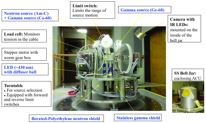
Figure 3: An overview picture of an ACU.

Each ACU is enclosed in a bell jar with 24-inch diameter and 30-inch height (Fig. 4). All ports on the bell jar are sealed with Viton-A o-rings. The bottom plate (5/8-inch thick, 35-inch diameter) of the bell jar supports the interior structure of the ACU. The underside of this plate seals to a 24-inch interface flange on the SSV lid. The weight of each ACU is about 314 kg. Access to the detector for each ACU is provided through a single port on the lid of the detector.

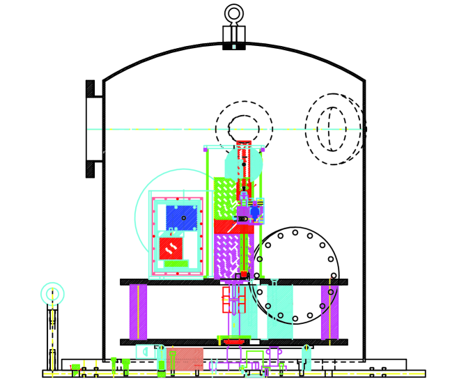
Figure 4: Sideview of an ACU.

3.2.1 Turntable

The interior body of the ACU is a stainless steel turntable consisting of two plates (known as top and middle plates) and three mechanically independent motor/pulley/wheel assemblies (known as deployment axes) mounted on the top plate. Each axis is capable of deploying a source (one of the radioactive sources or the LED) into the detector along the vertical axis (z-axis). The 5-inch separation between the two plates hosts the storage housing for the radioactive sources. The three axes are mounted with azimuthal separation of 120 degree, as illustrated in Fig. 5.

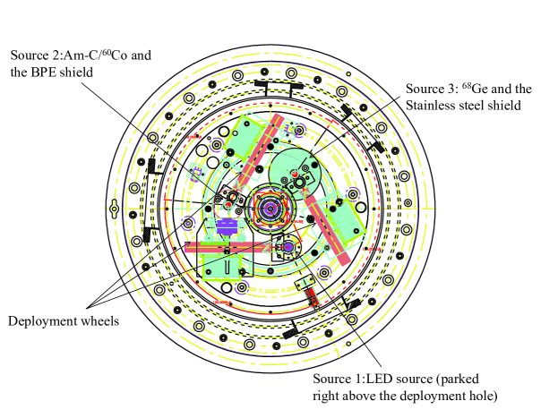
Figure 5: Topview of an ACU.

The turntable can turn clockwise or counter-clockwise by a stepper motor mounted at the center of the top plate. The center of each source is radially displaced from the center of the turntable by 114.5 mm. There is a 1-inch diameter hole at the same radial location on the bottom plate, aligning to a given penetration on the AD (see Fig. 2), through which the source can get deployed into the detector volume.

Mechanical details of a turntable are shown in Fig. 6.

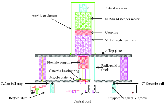
Figure 6: Drawing of a turntable.

A fixed stainless steel post is mounted at the center of the bottom plate, serving as the pivot of the rotation. A 2-inch high, 14-inch diameter stainless steel ring is mounted on the bottom plate. The top surface of the ring is a V-groove, hosting eight 0.5-inch ceramic balls (evenly spaced by a Teflon spacer ring). This assembly serves both as support to the turntable, as well as lubrication bearing to the turntable rotation. A NEMA34 stepper motor (Lin Engineering 8718M-16DE-01) coupled to a 50:1 straight gear box is mounted at the center of the top plate. The shaft of the gear box couples to the center post via a flexible bellow coupler (Wittenstein EC2 series). The shaft of the stepper motor extrudes from the back, on which an optical encoder is attached to to digitize relative rotation between the motor shaft and its body. A ceramic bearing ring (Champion Bearings Inc.) is mounted between the center post and middle plate for alignment. To limit the range of the rotation, a double-sided stop is mounted on the bottom plate. Two pushbutton style stainless steel limit switches (Schurter Inc.) are mounted on the underside of the middle plates to define the clockwise and counter-clockwise rotation limits (overall range 260 degrees).

Two radioactive sources in each ACU, when parked, are retracted into a 5-inch height, 2.25-inch thick cylinder (Borated polyethylene for ²⁴¹Am-¹³C/⁶⁰Co and stainless steel for ⁶⁸Ge) in between the top and middle plates to reduce background in the AD. A 2-inch thick, 3.25-inch diameter Borated polyethylene disk is located on the bottom plate right below the parked neutron source, serving as additional neutron shielding.

3.2.2 Radioactive source deployment axis

Fig. 7 shows details of a radioactive source deployment axis. It consists of a NEMA 23 173 oz-in stepper motor (Lin Engineering Inc. 5718M), a 60:1 right-angle worm gear-box (Rino Mechanical Components Inc, PF30-60NM), a 9-in acrylic deployment wheel with helical grooves, and a Teflon pulley assembly. An optical encoder is mounted at the back of the stepper motor to encode rotations of the motor shaft.

A flexible Teflon-jacketed stainless steel cable (McMaster Carr 3423T22, 0.026-in OD), one end attached to the wheel, is wound in the helical groove of the acrylic wheel. It then runs through a Teflon pulley assembly, and then attaches to the source assembly. When the stepper motor drives the acrylic wheel to unwind the cable, the source is deployed into the detector. Gravity from the source assembly keeps the cable vertically straight.

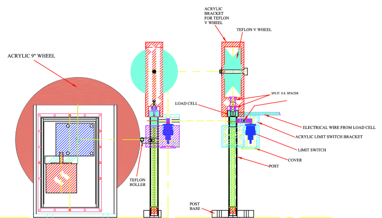
(a) Drawing.

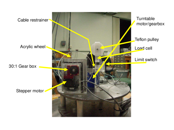
(b) Picture.

Figure 7: Drawing (a) and picture (b) of a single deployment axis.

3.2.3 LED source deployment axis

The design of the LED deployment axis is shown in Fig. 8.

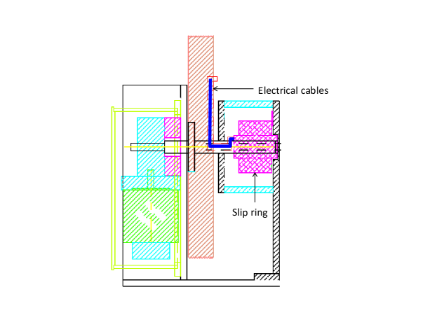
Figure 8: Drawing of the LED source deployment axis (pulley assembly omitted).

Due to the need to transmit electrical signals to the LED, the design of the LED deployment axis differs from that of radioactive sources in a few respects. It uses a miniature coaxial cable (Cooner Wire CW2040-3650 F, AWG 30 50 Ohm, 0.039-in OD) to both carry driving pulses, and serve as mechanical deployment cable. A LED driver (Sec. 3.3.1) is mounted inside the 9-inch acrylic wheel. A multi-wire electric slip ring (Moog AC6438-106) is mounted on a L-shaped bracket, which is fixed to the turntable. The rotary of the slip ring is attached to the shaft of the acrylic wheel. The slip ring carries input electric signals from the turntable to the LED drivers inside the wheel.

3.2.4 Failure protection

Numbers of protection features are implemented in the design of the source deployment system.

1. The gear box used in the driving unit is a worm gear which cannot be back-driven and is thus safe in case of power failure during a deployment.

2. Each source assembly consists of two weights, one above and one below the source, by which the tension in the cable is maintained (Sec. 3.3.4). It is critical to monitor this tension to avoid the following: a) tension that gets lost during the downward motion (bottoming out), causing the cable to unspool accidentally; b) source gets stuck during upward motion while the motor keeps turning and breaks the cable. A calibrated load cell (Honeywell Sensotec AL312-AT) is mounted below the Teflon pulley assembly. Source motion will be stopped immediately by the control software (Sec. 3.5) if the load cell value is outside the defined range. In case of bottoming out, the loss of tension due to the bottom weight signals the control system, while the top weight maintains sufficient tension in the cable.

3. The acrylic shields for the upper/lower weights and the source are all made into round-headed bullet shape (Fig. 17) to reduce the risk of the source getting stuck during upward motion.

4. A Teflon roller lightly presses against the acrylic wheel to retain the cable in the groove, while not adding too much friction to the rotation of the wheel. This further reduces the risk of accidental cable unspooling.

5. The turntable rotation is limited to a range of 260 degree by two Schurter limit switches to avoid overtwisting of electronic cables.

6. All motions are made conservatively slowly. The sources move at a speed of 7 mm/s, and the turntable rotates at a speed of 1.8 degree/s.

7. The upper limit of the motion is defined by the same Schurter limit switch as used on the turntable. When the upper weight hits a stop, it actuates the limit switch.

8. The breaking strength for the stainless steel cable is 18 kg, and that for the coaxial cable is measured to be 2 kg. To further reduce the risk of accidental breakage of cables due to excessive tension, the torque of the stepper motor (via a current limiting resistor on the motor driver) is limited to provide a maximum tension of 1.0 kg in the cable. All cables (including the coaxial cable for the LEDs) are tested to this value. In case the source got stuck and the load cell was malfunctioning, the stepper motor would “slip” (a mismatch between the stepping commander and the actual motion encoder) due to insufficient torque, upon which the control software would kill the motion.

9. The turntable motor torque is limited the same way. In case a limit switch was broken while “stop” was hit, the “slip” of the stepper motor would be detected by software.

10. The lower weight is made out of normal steel coated with Teflon, then enclosed in acrylic. In case of catastrophic cable breakage inside the AD, a rescue plan with a long rod and a permanent magnet could be developed.

3.2.5 Auxiliary components

For monitoring purpose, a CCD camera (Q-See QOCCD) with infrared lighting is mounted on the inner wall of the bell jar. The infrared lights can be kept on during normal detector operation, and present no effects to the PMTs inside the detector. Fig. 9 shows an image taken by the CCD camera.

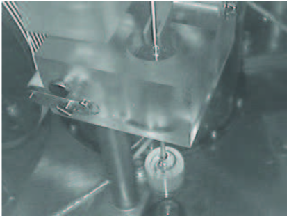
Figure 9: ACU CCD image during normal operation (source being stationary).

3.2.6 Materials

The source assemblies are in direct contact with liquid scintillator. Both the coaxial cable for the LED axis and the stainless steel cable are Teflon-jacketed. The upper/lower weights and sources are all enclosed in acrylic.

As shown in Fig. 3, motor/gear reducer assemblies for the turntable and source deployment axes are enclosed in acrylic housing. The CCD camera is also encapsulated in an acrylic shell. Teflon sleeves are used to cover all exposed non-Teflon electrical cables.

3.2.7 Flange interfaces, dry pipe, and leak checking

The ADs and ACUs, during normal operation, are immersed in ultrapure water in a water pool (an active muon veto detector). To be chemically compatible with ultra-pure water, all water seals are made with Viton-A o-rings. Standard ISO flange seals are adopted wherever applicable. As a requirement, after the final bolt tightening, all seals have to be separately checkable to a leak rate with an upper limit of $1.5\times 10^{-3}$ cc/s/atm for gas. Taking into account the fact that the viscosity of water is about a factor of 50 larger than that of common gases, and that the ACUs are located 2 m under water (0.2 atm), this limit translates to a water leak about 200 g/year, which can be easily taken away by evaporation under dry nitrogen environment.

Two types of leak checking techniques are employed in the ACU system: vacuum method (pumping out a volume) and pressure/sniffing using Freon and commercial sniffer. Despite the outgassing being an intrinsic background, the vacuum method generally has better sensitivity. The Freon sniffers, on the other hand, can also detect leak rate at $1.5\times 10^{-3}$ cc/s/atm, based on tests with calibrated leaks.

Flange interfaces on ACUs are illustrated in Fig. 10.

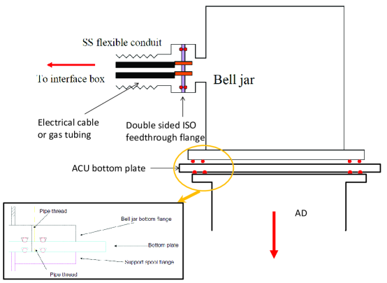
Figure 10: Illustration of seals on the ACU, with o-rings indicated by red circles.

The ISO flanges welded on the wall are sealed by double-sided electrical or gas feedthrough flanges. Outside the ACUs, the cables/gas lines run inside a so-called dry pipe system, shown in Fig. 11.

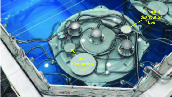
Figure 11: A picture showing the ACUs and dry pipe system on the AD lid.

The outer side of the feedthrough flange (facing away from the ACU) connects to a stainless steel flexible hoses (ISO63 or 100), which then connects to a stainless steel manifold chamber (known as the electrical or gas distribution box) where all cables or gas lines are consolidated. A stainless steel conduit assembly then takes all the cables and gas tubing out of the water pool. The double-sided vacuum feedthrough flanges allow the ACU and dry pipe system be leak checked separately. In addition, the AD would be protected by these vacuum feedthroughs even if a water leak was developed in the dry pipe system.

Details of seals below the ACU bell jar are shown in the inset of Fig. 10. The ACU bell jar seals to its bottom plate via a double o-ring seal, which then seals to the AD via another double o-ring seal. A 1/8-inch pumpout port is added between o-rings so that seals can be checked by pumping out the volume between o-rings.

All ACU side flange seals were leak checked by pressurizing each ACU to 1.25 atm (absolute) with Freon before the ACU gets installed onto the AD. After the ACU and cable installation, the entire dry pipe system is leak checked with 1.25 atm Freon. In this case, the open end of the dry pipe above water is sealed by a custom rubber seal designed at the Physical Science Laboratory at the University of Wisconsin with cables in situ. As a final check, the dry pipe is pressurized with 0.1 atm of nitrogen during the water filling when we looked for visible bubbles.

3.3 Calibration sources

To track and study detector response, multiple calibration sources are implemented in each ACU. Three deployment axes in each ACU can deploy, one at a time, a LED, ²⁴¹Am-¹³C/⁶⁰Co, or ⁶⁸Ge, into the detector. They emit light either at a given time with controllable intensity (LED), or at given gamma energies: 1.022 MeV (⁶⁸Ge), 2.506 MeV (⁶⁰Co), 8 MeV (²⁴¹Am-¹³C).

3.3.1 LED

Deployment axis 1 is designed to deploy a blue LED (Brite-LED BL-LUVB5N15C) with a 435 nm maximum wavelength. To make the light emission more diffuse, the LED is pocketed in a $\frac{3}{4}$ inch nylon ball. A miniature coaxial cable is soldered onto the LED and they get epoxied together with the nylon ball as shown in Fig. 12. The ball is then encapsulated in an acrylic enclosure with the cable going through the small hole on the top of the acrylic enclosure (see Fig.  12). The cable is wound into the grooves of one of the acrylic wheels.

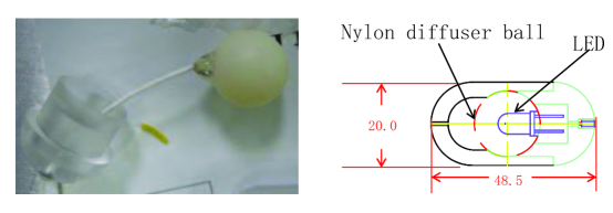
Figure 12: Left: picture of LED potted in the nylon ball; right: diagram showing the acrylic enclosure for the LED.

The driver of the LED follows the design in [17], also shown in Fig. 13. The light flash is triggered by a fast TTL pulse, with its intensity controlled by a negative DC voltage V_DC. The driver board is kept in a pocket inside the 9-inch acrylic wheel, with its output connected to the LED through the 5-meter long coaxial cable. An 100 nH inductor is in parallel with the coaxial cable on the driver. This inductor is essential to give a narrow ($\sim$10 ns) light pulse. As discussed in Sec. 3.2.3, the electrical signals get transmitted onto the driver board via the slip ring joint.

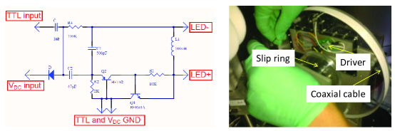
Figure 13: Left: schematics of the LED driver; right: picture of LED driver in the deployment wheel.

3.3.2 ¹³⁷Cs scintillator ball

During detector commissioning before liquid scintillator filling (“dry run”), it was desirable to use stable light source (LED light output intensity was found to be unstable at different locations) to scan the detector. We designed a special source made with ¹³⁷Cs deposited at the center of a spherical scintillator. ¹³⁷Cs primarily $\beta$-decays into ^137mBa ($T_{1/2}=2.552$ m), which has about a 10% probability of emitting K (624 keV) or L (656 keV) shell conversion electrons. The scintillation lights produced by these conversion electrons on the scintillator can be used as standard “candles”.

The design of the source is shown in Fig. 14, which was fabricated at the China Institute of Atomic Energy with 900 Bq of ¹³⁷Cs deposited. A picture taken when the source was being prepared for the dry run is also shown in Fig. 14.

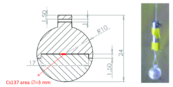
Figure 14: Left: design of the scintillator ball; right: real picture taken during dry run.

3.3.3 Radioactive sources

Deployment axes 2 and 3 host radioactive sources. The radioactive sources used in the calibrations are listed in Table 1.

Sources	Calibrations
Gamma source:60Co	Energy linearity, stability, resolution, spatial and temporal variations,
	and quenching effect. Gamma line energies: 1.173+1.332 MeV
Neutron source:241Am-13C	Gd neutron capture energy: $\sim$8MeV total gamma energy
Positron source: 68Ge	Energy scale, trigger threshold, and PMT QE(relative). Energy: 0.511+0.511 MeV

Table 1: Radioactive sources used in the ACUs.

The energy of the sources is in a range from 1 MeV to 8 MeV. Axis 2 is for deploying a combination of ⁶⁰Co (gamma) and ²⁴¹Am-¹³C neutron sources (see Fig. 15). The ⁶⁰Co source emits two gammas (1.173, 1.332 MeV) at about 100 Hz. Details of the ²⁴¹Am-¹³C neutron source will be discussed elsewhere [18]. In brief, $\alpha$-particles from a 28 $\mu$Ci ²⁴¹Am disk source impinge on a disk of compressed ¹³C powder and emit neutrons ($\sim$0.7 Hz) via $\alpha+^{13}\rm{C}\rightarrow\rm{n}+^{16}\rm{O}$. The neutron detection characteristics of the detectors can be thoroughly calibrated by the AmC source. The energy of $\alpha$s is attenuated by a gold foil (1 $\mu$m) to eliminate the production of excited states of ¹⁶O, thereby eliminating IBD-like background caused by correlated n-$\gamma$ emission. The residual backgrounds from ²⁴¹Am-¹³C are evaluated to be 0.2% compared to the IBD signals at the far site [9].

Axis 3 is responsible for deploying a ⁶⁸Ge source ($\sim$10 Hz). ⁶⁸Ge decays into ⁶⁸Ga with a $T_{1/2}$ of 271 days via electron capture. ⁶⁸Ga then $\beta^{+}$-decay into ⁶⁸Zn ($T_{1/2}=$67.7 minutes). Although ⁶⁸Ga is a positron emitter, the majority of the positrons emitted would annihilate in the source enclosure, making it effectively a gamma source with two 511 keV gammas. The positron detection threshold of the detectors can then be calibrated.

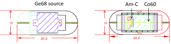
Figure 15: Acrylic enclosures for Ge68 (left) and AmC/Co60 (right).

3.3.4 Source assembly

As mentioned briefly in Sec. 3.2.4, to maintain sufficient tension in the deployment string to avoid accidental unspooling, each source is accompanied with two weights, one above and one below the source. Dimensions of the weight and its acrylic enclosure are shown in Fig. 16. Weld-on 3 acrylic cement from IPS was used to glue the enclosures.

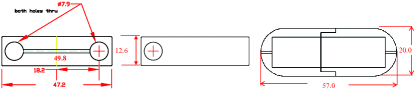
Figure 16: Top weight (left), bottom weight (middle), and their acrylic enclosures.

Details of the cable attachment scheme is illustrated in Fig. 17.

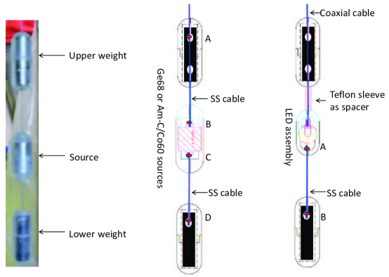
Figure 17: Left: picture of a complete source assembly. Middle and right: illustration of cable attachments for radioactive and LED source assemblies, respectively. Red spots indicate cable attachments. See text for details.

For strength considerations, we require that the cable attachments must only be constrained by stainless steel materials, not by the acrylic shell. To avoid stainless steel crimp cutting into the cable when improperly crimped, we adopted a method of looping the cable onto the attachment point, making a simple noose knot followed by two overhand knots, then potting the knots with epoxy. As shown in the middle sketch in Fig. 17, for a radioactive source, the upper weight and the source are connected through the deployment cable with two attachment points A and B. The lower weight and the source are attached through a separate stainless steel cable at points C and D. The cable attaches to a M3 nut at points A and D so the knot/nut can be trapped into the hole on the weight. For the LED source, the coaxial cable runs though the upper weight (no attachment) and then connects to the LED inside the acrylic shell. The distance between the upper weight and the LED shell is maintained by a 2.5-cm long Teflon sleeve. The lower weight attachment to the LED is the same as that for a radioactive source. Separations between source to both weights are maintained at $\sim$3 cm (tip to tip), and we keep a detailed database of as-built dimensions.

The entire weight of a source/weight assembly is about 110 g for the LED assembly, and 130 g for the other two.

3.4 Electronics and wiring

A large number of electronic components exists in each ACU, as summarized in Table 2.

Component	#/ACU	wires/component	details
Turntable motor	1	4	bi-polar motor in serial connection, A+/A-/B+/B-
Turntable encoder	1	8	differential readout (3 pairs) and digital 5 V power (1 pair)
Deployment axes motors	3	4	bi-polar motor in serial connection, A+/A-/B+/B-
Deployment axes encoder	3	8	differential readout (3 pairs) and 5 V power
Turntable limit switches	2	2	single pole single throw
Deployment axes limit switches	3	2	single pole single throw
Deployment axes load cells	3	8	isolated 5 V supply to load cell (1 pair), +12/-12 V input to amplifier (1 pair), 2 pairs of redundant voltage outputs
CCD camera	1	4	12 V input power (1 pair), output (coaxial)
LED driver	1	4	TTL input (coaxial), VDC (1 pair)

Table 2: Electronics components and wiring requirements for each ACU.

We shall discuss details of these instrumentation and their wiring I/O in this section.

3.4.1 ACU internal electronics and wiring

In Fig. 18, a picture of wiring connections inside an ACU is shown.

Figure 18: ACU internal wiring picture taken during ACU assembling. The breakout boards, 12-conductor cables (red), and the MDC feedthrough can be seen from the pictures.

A custom double-sided ISO100 vacuum feedthrough flange (MDC Inc.) hosting two mil-spec 52-pin feedthroughs and two isolated BNC feedthroughs is used on each ACU. One of the BNC connections carries the CCD camera image signals, and the other carries the TTL trigger signals for the LED. The signals from individual components get consolidated by two breakout boards located inside a shielded metal box mounted between the two turntable plates. Each board breaks into four 12-conductor (AWG 22 shielded twisted pairs) cable, grouped by a single 55-pin female mil-type connector, mating to the male connector on the MDC flange.

A cable guiding post is mounted on the turntable. From the breakout box, all 12-conductor cables are cable-tied to this post running upward. The cables then run through a rotatable shackle mounted on the underside of the bell jar dome, then go horizontally to connect to the feedthrough flange. This routing scheme, shown in Fig. 19, ensures that cables do not run into other mechanical components when the turntable is rotating.

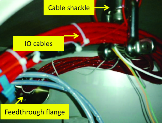
Figure 19: A picture taken when ACU internal cable connection is made to the feedthrough flange.

Most signals simply pass through the breakout boards. The load cell signals are exceptions, as the raw signals from them are of the order of mV (raw sensitivity = 2 mV/lb with 5 V power input). To avoid noise pickup (which may swamp the raw signal), these signals have to be amplified in-situ before getting transmitted to the readout electronics. Non-inverting amplifiers were implemented on the breakout boards using op amps (AD843) operating under negative feedback mode (Fig. 20).

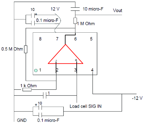
Figure 20: Schematic diagram of the load cell amplifier circuitry on the breakout board.

Capacitors at the power inputs as well as at the output are essential to suppress noise pickup during motor movement. It was also found that the 5V power GND to the load cell has to be isolated from the analog ground (defined by the $\pm$12 V GND to the opamp). To avoid loss of load cell output due to op amp failure, two redundant amplifier circuitries were implemented for each load cell.

3.4.2 External electronics and wiring

The ACUs are mounted on the lid of the AD inside the water pool during normal operation. ACU cables ($\sim$60 m) have to go all the way from the MDC feedthrough flange to the control electronics and computers located in the electronics room. Under the water, cables are sealed from the water by a stainless steel dry pipe system (Sec. 3.2.7). For each ACU, two 48-conductor cables (24 individually shielded twisted pair, AWG22) and two RG58 coaxial cables connect to the two mil-spec and two BNC feedthroughs on the MDC flange respectively.

The central hub for the ACU cables in the electronic room is a 4-U power/signal distribution box, one for each ACU, known as the ACU control box. A simplified schematic diagram of the box is shown in Fig. 21. The stepper motor wires connect to its driver (E-DC by Parker Inc.) first. The power to the driver is supplied by a 24 V DC power supply. As mentioned in Sec. 3.2.4, output current limits on these drivers were set by an adjustment resistor to limit the output torque from the stepper motors. An interface board (National Instruments UMI 7764) collects wires from the E-DC driver, the optical encoder, as well as the limit switches, and consolidates all motion I/O signals through its 68-pin connector, to be connected to the National Instrument motion control card PCI 7358. The control box also hosts three independent isolated 5 V power supply for the three load cells, as well as the $\pm$12 V power for the op amp and the CCD camera. The amplified load cell signals pass through the control box going into the ADC (National Instruments PCI 6224), whereas a DAC (National Instruments PCI 6703) passes a DC voltage through the ACU control box to the LED driver.

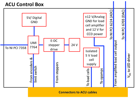
Figure 21: Schematic of the ACU control box.

The motion control card National Instruments PCI 7358 also contains several digital outputs (TTL). To avoid stepper motors introducing noises in detectors, solid state relay chips (ASSR-1511, schematics shown in Fig. 22) are implemented in the control box to allow remote turning off of all motor driver’s power when the source is deployed in position. The same relays are used in the control box to switch on/off the CCD camera, LED control voltage etc.

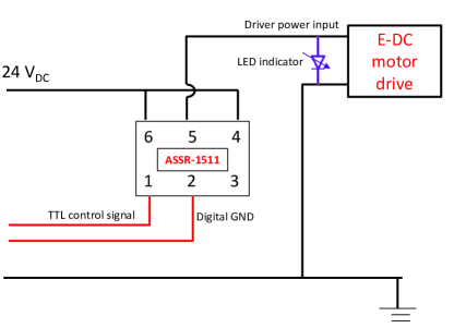
Figure 22: Schematic of solid state relay circuitry in the control box to control power to the stepper motor drive.

The TTL trigger signals for the LED are generated by National Instruments PCIe 6535 DAQ card, which get carried by a RG58 coaxial cable going directly to the ACU. A copy of this TTL trigger gets fed into a TTL-LVPECL converter, which then gets input to the local trigger board (LTB) of the front end electronics. During the LED calibration runs, the LTB only triggers on this external trigger. The signal cable from the CCD camera, also RG58, runs into a video IP PCI card (Q-see), video streams of which then get displayed on the computer.

Commercial PCI extension crates (Magma), a 7-slot one for each near site, and a 13-slot one for the far site, host all the PCI cards mentioned above. A server (Supermicro) with dual power supply running WindowsXP SP3 and LabVIEW 8.5 is installed in each experimental hall, communicating with all the automation hardware and sensors through the PCI crate. UPS power is in service to the computer and Magma crate to ensure that the system can shut down properly during power outage.

3.4.3 Groundings

An effective practice to avoid ground loops in electronics is to derive all grounding connections from a single point. Efforts have been made to ensure that the electronic ground of all PMTs in the AD is defined only by the Cu grounding bar in the electronic room (known as the clean ground). The stainless steel tank is connected to the clean ground via a dedicated grounding braid and is insulated from everything else. The electronic components inside the ACUs follow the same guideline. Their grounds are defined by the control box ground (shorted to clean ground in the electronic room) via individual grounding wires inside the 48-conductor ACU cable, and electrically insulated from the bell jar and turntable. The shielding braids of all twisted pairs between the ACU and control box are grouped together, shorted to the clean ground at the control box end, and cut at the ACU end.

3.5 Design of the control software

In the design of the control software, balancing safety and automation has always been the main focus. From the safety point of view, the control software has to prevent or stop operations which can cause harm to the system, while, to achieve genuine automation, it cannot completely rely on human intervention when potentially dangerous situations arise. However, whenever there is a conflict, safety always comes first at the expense of automation.

3.5.1 Design

The control software consists of several application modules written in LabVIEW. This modular (as opposed to monolithic) nature of the software minimizes coupling between parts and simplifies the customization for each site. The central piece is the Main Program which consists of two independent but coupled parts (or loops). Each performs a crucial function: the “Monitor Loop" periodically monitor sensor readings and the “Control Loop" direct signals to the electronics to control source motions. The Main Program also provides the main interface for user operation. The Data Fetcher fetches readings from the sensors, e.g. load cells, encoders, etc., and provides such readings to the main program. The Watchdog ensures that the Main Program always duly performs its monitoring function. The Distributed Information Management (DIM) Communication Module relays information between the main program and the data-acquisition system (DAQ) over TCP/IP, enabling automatic deployment. The detailed workings of the software will be discussed below from a functional point of view.

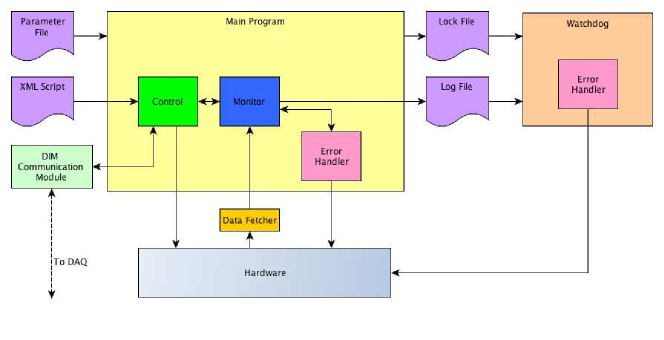
Figure 23: Schematic of software structure.

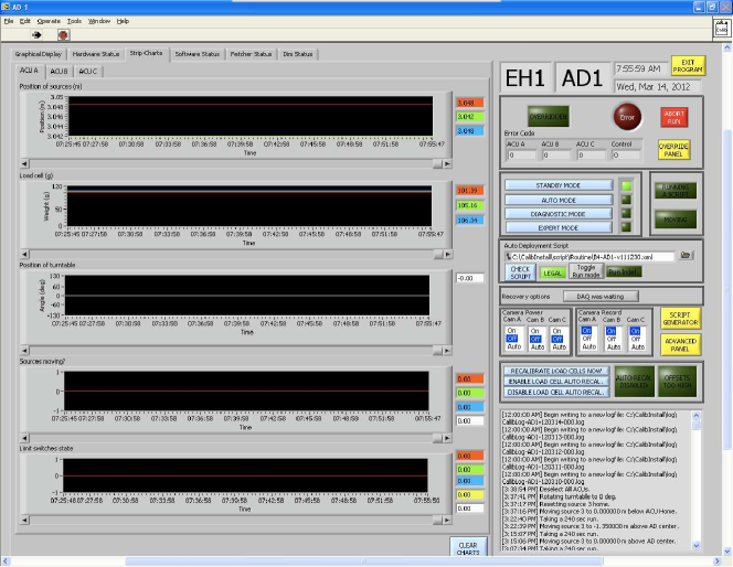
Figure 24: Screenshot of the Main Program.

3.6 Monitoring

Involved in the monitoring function of the software are the Monitor Loop in the Main Program, the Data Fetcher and the Watchdog. The Data Fetcher fetches readings from all sensors (See Table 3 ) from the hardware at the highest possible frequency allowed under computer and hardware constraints. The readings are then transmitted to the Main Program via a local DataSocket server. On receipt of the readings, the Monitor Loop will look for signs of danger and issue alarms if any such signs are observed (see Table 4). When an alarm is issued, the Main Program would signal all motors to stop and would then power them down via the relay circuitry in Fig. 22. After processing this set of readings, the Main Program would then signal the Data Fetcher to clear the latched set of readings and read in another set. Such a cycle typically runs at 1 to 2 Hz.

Variable name	Axis	Type	Unit
Stepper count	All	Int	Counts
Encoder count	All	Int	Counts
Load cell reading	All	Double	Volts
Motion status	All	Bool	-
Reverse limit switch status	All	Bool	-
Forward limit switch status	Turntable	Bool	-

Table 3: Sensor readings from each ACU.

Bit	Name	Remarks
1	Turntable stepper/encoder mismatch	Tolerance = 0.6 deg
2-4	Source 1-3 stepper/encoder mismatch	Tolerance = 2.5 mm
5-7	Source 1-3 reaches maximum depth	IAV bottom or OAV bottom
8-10	Source 1-3 load cell out of limit	below 50% of or 300 g above nominal weight
11	Source moves when turntable is misaligned	Prevent misoperation
12	Turntable moves when some source is deployed	Prevent misoperation
13	More than one motor move simultaneously	Prevent misoperation
14-18	Inconsistent status	Ensure internal consistency
19-21	Load cell saturated	Load cell offset $<$ -9.0 V

Table 4: Alarms that can be issued by the Main Program

To provide an additional layer of security, the Monitor Loop is constantly watched over by the Watchdog, making sure that the Main Program is running and updates the log file at a fixed frequency (typically 1 Hz). An alarm will be issued when this frequency is not met.

3.6.1 Control

The Control Loop of the Main Program provides 3 modes of operation: Manual, Diagnostic and Auto, for controlling the four axes (1-3 for deployment axes and 4 for turntable) of motion for each ACU, and the voltage and frequency of the LEDs. The Manual mode is restricted to expert use for non-standard deployments. Any possible operation can be performed unless forbidden by the Monitor Loop. Unlike the Manual mode which requires point-and-click by the user, the Diagnostic mode and the Auto mode accept an XML script which specifies the sequence of operations to be performed. In Diagnostic mode, the Control Loop simply performs each operation in the XML script sequentially until the end of the file. In the Auto mode, the Control Loop and the Daya Bay DAQ system communicate via DIM. Both systems publish their status on a dedicated DIM server, and listen to the other side with a handshaking protocol depicted in Fig. 25.

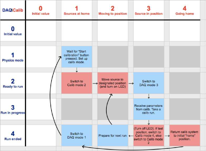
Figure 25: Communication protocol between the control software and DAQ. See text for details.

Control Loop listens to the DAQ for the shifter’s "Start" signal before deploying any source. The Control Loop signals the DAQ to start a run when the source reaches the designated position and the DAQ would reply to the Control Loop when the DAQ run is done. The Control Loop then executes the next command (if there is any) in the XML script, performs the above “handshake" and repeats until the end of the XML script, at which point the Control Loop informs the DAQ of the end of calibration and returns to the initial state. When an error occurs during Auto mode, the DAQ would be notified, and after recovery the calibration can resume from the place where it left off without any intervention from the DAQ side in most cases. By this means, after the shifter commences the weekly calibration program, the entire program (typically 5 hours by deploying three sources in each ACU, one at a time, 3-5 stop per round trip) in all three halls and eight ADs are executed simultaneously with fully automated data taking at one data run per source stop in each hall.

3.6.2 Notification and Logging

There are several channels employed in the software for notification. When an alarm is issued, the Main Program would signal the detector-control system (DCS) via DIM, which notifies the shifter. On the other hand, the Main Program would also send an email notification to the experts with a summary of alarms issued (Table 4) and recently executed commands, hence expediting the recovery process. While all sensor readings are saved onto the local disk, only a subset of monitoring-related readings would be saved in the DCS database, and another subset of control-related readings are saved to the online database via DAQ.

4 Quality controls and position calibration

4.1 Mechanical reliability tests

Daya Bay experiment is planned to run for at least three years, and the automated calibration units would run on a weekly basis over this period. This amounts to at least 156 full calibration cycles for each ACU. We constructed in total 25 (24 and a spare) ACUs. To ensure the robustness of each ACU, longevity tests were undertaken at Caltech before shipping to Daya Bay. The longevity test involves running the ACU for 200 consecutive full deployment cycles. Each cycle involves deploying each of the three sources to a distance corresponding to the detector center, and then retracting to the origin. Each cycle takes about half an hour, and a complete longevity test for each ACU takes about four days. No noticeable damage has been found in any of the parts after the longevity test.

Two different stress tests, which emulate situations where parts of ACUs are damaged, were also performed. One stress test, dubbed the “extreme test", targeting the limit switch and the load cell, involves forcefully pulling the source assembly against a disabled limit switch until the stepper counts gets out-of-sync with the encoder counts. This forceful pull was repeated at least 200 times for each of the axes. The objective of this test was to make sure that the functionality of the limit switch and the load cells would not be affected under such an extreme condition. The other, called “load test", aimed at ensuring secure attachment of the sources, involves hanging a weight of about 1 kg (max possible pull from the motor) from the source assembly for a duration of at least 15 minutes. No source ever failed any of these tests.

4.2 Position calibration

Source deployment positions are required to have an accuracy of 0.5 cm. The elongation of the stainless steel wire due to the weight of the sources is negligible, so the positional accuracy is primarily determined by the accuracy in the diameter of the acrylic wheel. There are also some small effects coming from the depth of the grooves into which the wires are wound and the alignment between the deployment wheel and the auxiliary wheel. Given that a deployment to the center of the detector typically requires 4 turns of the wheel, uncertainty in the deployment length can be an order of magnitude greater than that of the wheel diameter. Therefore, a sub-mm uncertainty in the wheel diameter can possibly jeopardize our required accuracy. We devised a method to precisely estimate the effective diameter of the wheel. We constructed a calibration ruler, with accurately measured marks, aligned along the source deployment axis. The positions of the source can then be compared with the marks on the ruler. Hence, an effective diameter of the wheel can be estimated accurately with a linear fit.

The calibration ruler is made of a roughly 6 m long Teflon coated stainless steel wire, with a 50 g weight attached to one end. Six crimps which served as calibration marks were attached at various measured positions on the wire. The ruler was then lowered into a mock-up detector, a 5.5 m long acrylic tube, on which we marked the positions of the crimps. We then offset the ruler by 200 mm, and a different set of calibration marks were similarly translated onto the tube. We also used the top surface of the turntable as a calibration point.

For each axis, the source was first deployed close to each calibration mark. The source was then made to inch along the axis in steps of about 0.1 mm. The encoder counts of the source motor was recorded when the source was flush with the calibration mark.

The data were then subject to a linear fit of the form $y=kDx+C$, where $k=\frac{\pi}{4000\times 60}$ (4000 is the encoder count/resolution, and 60 is the gear ratio), x and y are respectively the encoder counts and position of calibration marks, and the fit parameters D and C are respectively the wheel diameter and the offset. Fig. 26 shows the distribution of wheel diameters with an average at 227.7 mm. Most of the wheel diameters are in good agreement within 1 mm, except that for ACU5A axis 3, which has a $\sim$3 mm smaller diameter compared to the rest due to machining. One also observes from Fig. 26 that on average the effective diameter for axis 1 is $\sim$0.4 mm larger than those for axes 2 and 3, which is consistent with the different diameters of the deployment cables (0.039-in for LED, 0.026-in for radioactive sources).

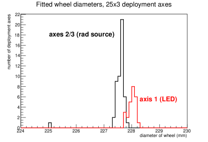
Figure 26: Effective wheel diameters of all 25$\times$3 ACU axes obtained by the position calibration.

The parameters thus determined are used to compute the expected position at each encoder reading. For demonstration, differences between the expected and actual position on the ruler for ACU1A, deployment axis 1, are shown in Fig. 28 as a function of vertical deployment length, in which the remaining scattering of the difference (RMS) is used as a measure of the position accuracy for each deployment axis. The distribution of the position accuracy thus determined for all 25$\times$3 deployment axes (including those on the spare ACU) is shown in Fig. 28. Conservatively, we take $\sim 2$mm as an estimate of the position accuracy of the calibration source to its limit switch. As a final cross check, obtained wheel diameters were input into the control software, and each source was deployed to the nominal AD center in the mock detector. The position of the source and the marker on the ruler agree within 3 mm.

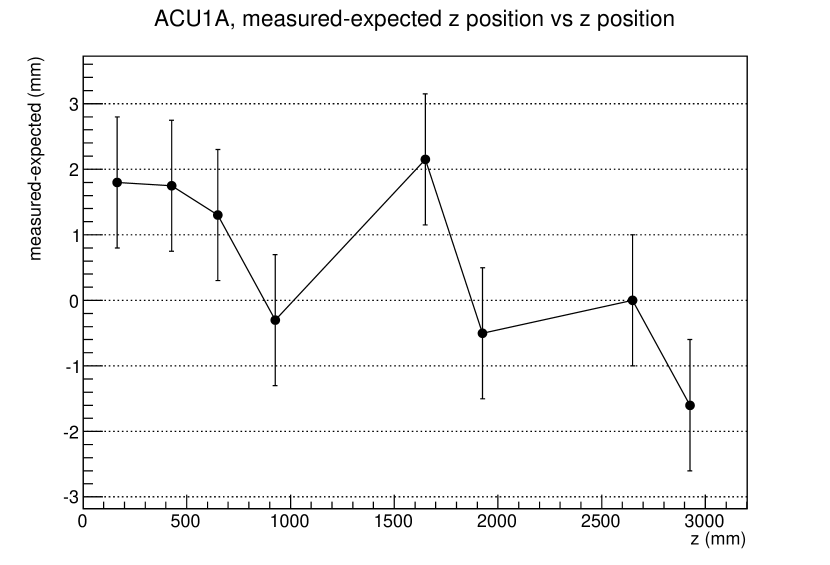
Figure 27: Difference between the expected (software) and true position, ACU1A source 1.

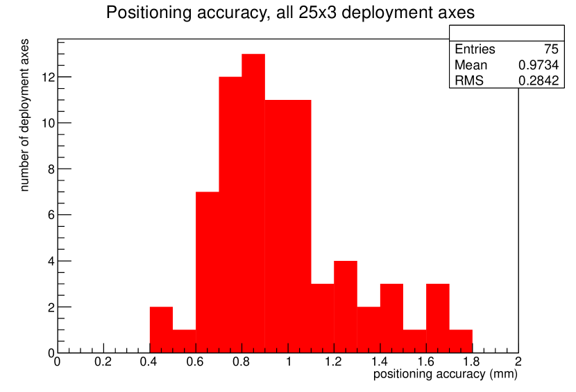
Figure 28: Extracted position accuracy (based on the non-zero scattering in Fig. 28 for all deployment axes.

The absolute source accuracy of a deployed source within an AD is estimated as follows. The position calibration demonstrated in Fig. 28 is for the source-limit switch distance in the vertical direction only. Inside an AD, we must include the accuracy of 1) ACU mounting position relative to its support flange, 2) the AD verticality, and 3) the position of the ACU support flange relative to the general AD coordinate. The accuracy in 1) is $\sim$ 2mm in horizontal plane, given the size of bolt holes on the ACU bottom plate. The accuracy in 2) and 3) arises from the AD survey data [19], which translate to an absolute accuracy of $<$1 mm in x, y, and z coordinates. Combining everything in quadrature, we reach a final $\sim$4 mm position accuracy of a source in the AD.

5 Performance of the calibration system

The performance of the antineutrino detector with calibration sources has been thoroughly described in Ref. [11]. In this section, we will show results more directly related to the performance of the calibration system.

5.1 Motion/sensor performance

All ACUs have been fully functional since the beginning of Daya Bay data taking in August 2011. Alarms only occur at a rare rate of $\sim$ 2-3 per week for the entire system. All these alarms were identified as sensors picking up transient noise, in particular during motor movement a load cell readout picked up noise once in a while that triggered the alarm.

The load cell reading during a typical source deployment is depicted in Fig. 29. As the source goes down and crosses the liquid boundary, there is a change of tension in the load cell by about 30 g due to the buoyant force applied onto the weight/source assembly. After the source is fully immersed, the load cell tension gradually increases as more cable unspools and adds to the weight felt by the load cell. Once the source is at its target position, it stops and the data taking starts. When the data have been taken, the motor reverses direction to extract the source from the AD. Typically there will be a sudden increase in load by about 10 g, corresponding to an additional dynamic friction that has to be overcome. One then sees a gradual reduction of the load due to less and less cable weight until the weight/source assembly crosses the liquid level again when the tension will recover more or less to the orginal level due to the loss of buoyant force. Right after the source leaves the liquid, the liquid will be dropping back into the detector, causing another small decrease of the load. The program will then reset the motor home by moving the source up till the top weight activates the limit switch, at which point there is a spike in the load cell. The source then moves down by 5 cm and get “parked”. Even when the source is parked, the load cell tends to pick up some noise when other motors are moving, with a typical noise level of a couple of grams, as shown in Fig. 29.

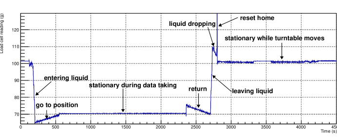
Figure 29: Strip chart of a load cell reading for a corresponding source going into and out of the liquid.

5.2 Calibration runs during the AD dry run

The LED source and the ¹³⁷Cs scintillator ball played an important role in commissioning the detector, in particular the “dry run” before the liquid scintillator filling.

LEDs can be used to mimic real particle interactions to study detector electronics. In Fig. 30, measured total charge from an LED intensity scan in an AD is shown. One sees that one could easily adjust the control voltage to simulate gamma-like low energy events to muon-like high energy events, given a typical AD energy scale of 160 PE/MeV [11]. Low energy events allow precise determination of PMT gains, and the high energy events allow one to study effect of PMT/electronics after a large pulse, e.g. baseline overshoot, ringing and recover, as well as retrigger issues.

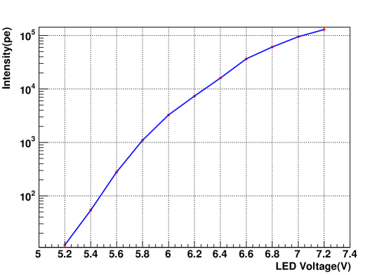
Figure 30: Detected light intensity (in number of PE) as a function of LED control voltage.

Narrow timing distribution of the LED flashes relative to the trigger signal is an important requirement for using the LED as a timing calibrator, in particular the rising edge of the light pulse. In Fig. 31, the TDC distribution of a PMT channel (relative to the trigger signal generated by the TTL command pulse) is plotted for a high (black) and low (red) light intensity run. The sharp (RMS 0.9 ns) distribution in the former demonstrates that the emitted light pulse has a very sharp rising edge. The timing calibration data for all ADs were collected with LEDs under high intensity.

The TDC spectrum in the low intensity run reveals the overall emitted photon timing distribution. The primary pulse has a FWHM of 5 ns. A small late light tail of duration about 25 ns from the initial edge can also be observed from the distribution. The timing difference between the two distributions is caused by timing walk from the discriminator in the electronics.

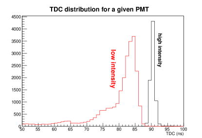
Figure 31: TDC distribution of a PMT during a high (black) and low (red) LED intensity run.

Despite these good characteristics, we discovered that due to different amount of coaxial cable winding on the spool, the LED intensity would change a few percent as a function of position. Therefore, to characterize the dry detector response, position dependent uniformity in particular, a ¹³⁷Cs scintillator ball was designed as a stable “candle” (Sec. 3.3.2). In Fig. 32, the measured total charge spectrum with the scintillator ball deployed at the detector center is shown, in which a clear conversion electron peak can be observed at around 90 photoelectrons.

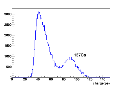
Figure 32: ¹³⁷Cs scintillator ball spectrum in a dry AD.

5.3 Radioactive sources calibration in-situ

The ²⁴¹Am-¹³C/⁶⁰Co and ⁶⁸Ge source spectra in a full AD are shown in Fig. 33. Low energy shoulders due to dead material on the source assembly are visible on both spectra. The full absorption peak around 2.5 MeV in the ⁶⁰Co spectrum is the primary method of calibrating the PE to MeV conversion factor from ADs. The low energy peaks on the spectrum were identified as gamma lines from ²⁴¹Am (662, 722 keV). The neutron-Gd capture gamma peak is also clearly observed around 8 MeV. Since the decay rate of ⁶⁰Co dominates (100 Hz vs 0.7 Hz of Am-C), the n-H capture from the Am-C source will produce negligible bias to the ⁶⁰Co energy (nor can it be identified due to the energy resolution). The variations of the energy scale among all six ADs have been controlled within 0.5% [11]. Some ⁶⁰Co contaminant was found in ⁶⁸Ge, which may come from imperfect control of the fabrication environment. However it does not affect effective application of this source.

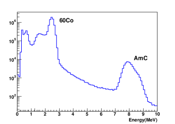
(a) AmC-⁶⁰Co

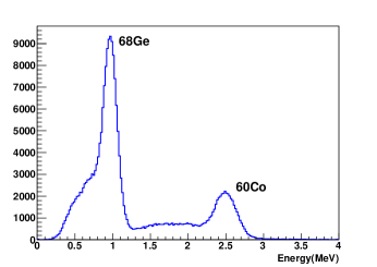
(b) ⁶⁸Ge

Figure 33: Energy spectrum of the ²⁴¹Am-¹³C/⁶⁰Co source (a) and the ⁶⁸Ge source (b) when deployed at the AD center.

Accurate knowledge of the true position of the ACU sources provide stringent constraints to the vertex reconstruction as well as vertex based energy correction. Fig. 34 shows the reconstructed position (with a charge pattern based algorithm) in $z$ and $r^{2}$ of ⁶⁰Co source for all three ACUs at $z=0$ (center).

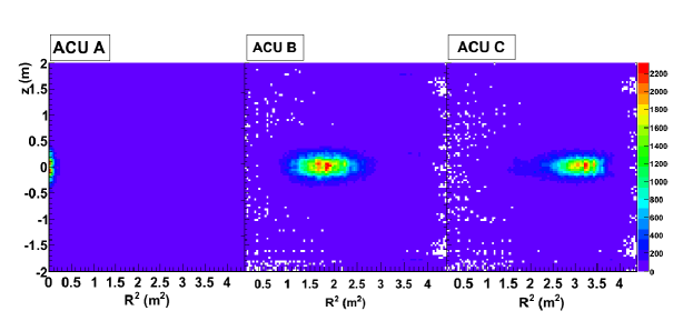
Figure 34: Reconstructed ⁶⁰Co source position in a near site AD. Y axis: z position of the source with AD center being z=0. X axis: r² position of the source with AD center being r${}^{2}=0.$

The projections of reconstructed to true position difference in $x$, $y$ and $z$ are shown separately for the three runs in Fig. 35.

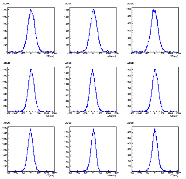
Figure 35: Difference in the reconstructed to true position of the ⁶⁰Co source deployed to $z$=0 for the three ACUs.

Studies are ongoing to reduce the reconstruction bias and to improve the resolution.

6 Summary

In this paper we describe the design and performance of the automated calibration system for the Daya Bay Reactor Neutrino Experiment. This system consists of 24 functionally identical pulley/wheel and stepper motor assemblies, each designed and constructed as a precise and reliable robotic unit, capable of deploying three difference sources vertically into detectors in a fully automated fashion. The Daya Bay Neutrino experiment has been in smooth full scale operation, and has provided the first unambiguous measurement of neutrino mixing angle $\sin^{2}(2\theta_{13})$. This fully automated system has provided a powerful and robust tool to monitor and calibrate the detector response at different positions in the detector, therefore giving a tight control on the uncertainty of the energy scale. In the remaining lifetime of the experiment we will continue using the system to help measure the neutrino rate and spectra shape from all eight detectors, targeting to a final precision <0.01 (90% confidence level) to $\sin^{2}(2\theta_{13})$, and put tighter constraints on $\Delta m_{13}^{2}$ and the reactor neutrino spectrum.

The calibration system reported in this paper is uniquely designed within difficult size, material, automation, reliability, and interface constraints. The successful operation of this system provides precious experience to similar detectors where regular, remote, and automated calibration accesses are necessary.

7 Acknowledgments

This work was done with support from the US DoE, Office of Science, High Energy Physics, the US National Science Foundation, the Natural Science Foundation of China Grants 11005073 and 11175116, the Shuguang Foundation of Shanghai Grant Z1127941, and Shanghai Laboratory for Particle Physics and Cosmology at the Shanghai Jiao Tong University.

The authors gratefully acknowledge the strong technical support of R. Cortez, J. Pendlay, and A. Raygoza of the Kellogg Radiation Laboratory at Caltech. This paper is dedicated to the memory of Ray Cortez, who had been a primary designer and chief machinist of this system. We acknowledge numbers of summer intern students from Caltech and Shanghai Jiao Tong University who had contributed to the design, fabrication, and installation of this system. We thank Xichao Ruan and his colleagues from Chinese Institute of Atomic Energy for providing radioactive sources to the system, and the DAQ and Slow Control group from the Institute of High Energy Physics for implementing interfaces to the calibration software. We are grateful to the rest of the Daya Bay collaborators, particularly Jeff Cherwinka from University of Wisconsin for his continuous professional engineering support throughout the years. We thank the Daya Bay on-site installation team for their dedicated work.

References

- [1] J. Beringer et al. (Particle Data Group), Phys. Rev. D86, 010001 (2012)
- [2] R. D. McKeown and P. Vogel, Phys. Rept. 394, 315-356 (2004)
- [3] B. Pontecorvo, Sov. Phys. JETP 6, 429 (1957); 26, 984 (1968).
- [4] Z. Maki, M. Nakagawa, and S. Sakata, Prog. Theor. Phys. 28, 870 (1962).
- [5] K. Abe et al. (T2K Collaboration), Phys. Rev. Lett. 107, 041801 (2011).
- [6] P. Adamson et al. (MINOS Collaboration), Phys. Rev. Lett. 107, 181802 (2011).
- [7] Y. Abe et al. (Double Chooz Collaboration), Phys. Rev. Lett. 108, 131801, Phys. Rev. D 86, 052008 (2012)
- [8] J. K. Ahn et al. (RENO Collaboration), Phys. Rev. Lett. 108, 191802 (2012)
- [9] F. P. An et al. (Daya Bay Collaboration), Phys. Rev. Lett. 108, 171803 (2012), Chinese Physics C37, 011001 (2013)
- [10] X. H. Guo et al. (Daya Bay Collaboration), arXiv:hep-ex/0701029.
- [11] F. P. An et al. (Daya Bay Collaboration), Nucl. Instrum. Meth. A685, 78-97 (2012)
- [12] M. Apollonio et al. (CHOOZ Collaboration), Eur. Phys. J. C27, 331-374 (2003).
- [13] F. Boehm et al. (Palo Verde Collaboration), Phys. Rev. D62 072002 (2000).
- [14] J. Goett et al., Nucl. Instrum. Meth. A637, 47-52 (2011)
- [15] J. Boger et al. (SNO Collaboration), Nucl. Instrum. Meth. A449, 172-207 (2000)
- [16] http://www.ni.com
- [17] J. S. Kapustinsky et al., Nucl. Instrum. Meth. A241, 612-613 (1985).
- [18] Jianglai Liu et al., in preparation.
- [19] Jeff Cherwinka et al., Daya Bay Technical Doc # 5819