The abundance of H₂O and HDO in Orion KL from Herschel/HIFI

Abstract

Using a broadband, high spectral resolution survey toward Orion KL acquired with Herschel/HIFI as part of the HEXOS key program, we derive the abundances of H₂O and HDO in the different spatial/velocity components associated with this massive star-forming region: the Hot Core, Compact Ridge, and Plateau. A total of 20 transitions of H₂¹⁸O, 14 of H₂¹⁷O, 37 of HD¹⁶O, 6 of HD¹⁸O, and 6 of D₂O are used in the analysis, spanning from ground state transitions to over 1200 K in upper-state energy. Low-excitation lines are detected in multiple components, but the highest-excitation lines ($E_{u}>$ 500 K) are well modeled as emitting from a small ($\sim 2^{\prime\prime}$) clump with a high abundance of H₂O ($\chi=6.5\times 10^{-4}$ relative to H₂) and a HDO/H₂O ratio of 0.003. Using high spatial resolution ($1.5^{\prime\prime}\times 1.1^{\prime\prime}$) images of two transitions of HDO measured by ALMA as part of its science verification phase, we identify this component as located near, but not directly coincident with, known continuum sources in the Hot Core region. Significant HDO/H₂O fractionation is also seen in the Compact Ridge and Plateau components. The outflowing gas, observed with both emission and absorption components, has a lower HDO/H₂O ratio than the compact components in Orion KL, which we propose could be due to modification by gas-phase shock chemistry.

1 Introduction

Water is a central molecule in the physics and chemistry of the interstellar medium (van Dishoeck et al., 2011; Bergin & van Dishoeck, 2012; Melnick, 2009; Caselli & Ceccarelli, 2012). In the cold, dense stages of star formation, water is often the dominant constitutent of the ice mantles that harbor most of the heavy atoms (Gibb et al., 2004; Öberg et al., 2011) and therefore plays a significant role in the formation of the rich organic molecular inventory that is believed to result largely from chemistry on grain surfaces (Herbst & van Dishoeck, 2009). In warmer regions ($T>100$ K), the ice mantles evaporate and water can be one of the major gas phase constituents behind molecular hydrogen. Finally, at very high temperatures ($T>400$ K), gas-phase reactions of atomic oxygen with H₂ can convert all oxygen not in CO into water on fast timescales (Kaufman & Neufeld, 1996; Bergin et al., 1998). Due to its high dipole moment, gas-phase water can be detected through strong transitions in the submillimeter and infrared that are important in the energy balance of the molecular cloud (Neufeld et al., 1995). The HDO/H₂O abundance ratio is also a powerful diagnostic of the evolution of star-forming regions, due to the strong sensitivity of deuterium fractionation processes to physical conditions, particularly temperature (Millar, 2003). This ratio is posited as a tracer of the possible link between interstellar and cometary water, holding implications for understanding the mechanism for the delivery of water to the young Earth (Bockelée-Morvan et al., 1998; Hartogh et al., 2011; Caselli & Ceccarelli, 2012). Furthermore, observations suggest that the chemistry leading to the deuteration of H₂O is very different from that of other organic molecules such as HCN, H₂CO, and CH₃OH (van Dishoeck et al., 2011).

The Orion Kleinmann-Low nebula (Orion KL) is the nearest massive star-forming region, at a distance of 414 $\pm$ 7 pc (Menten et al., 2007), with very strong gas-phase water emission in the submillimeter and infrared. Studies of gas-phase H₂O from ground-based observatories are limited by atmospheric absorption of the most emissive transitions at the typical temperatures of molecular clouds. Most of the exceptions are lines that exhibit maser activity in Orion KL (Genzel et al., 1981; Menten et al., 1990; Cernicharo et al., 1990, 1994, 1999; Hirota et al., 2012), and so have limited usefulness in characterizing the bulk water abundance. Therefore, water has been a key focus of space-based observatories in the far-infrared. The ground state ortho transitions ($1_{10}-1_{01}$) of H₂O and its isotopologues were measured with a few arcminute beam by the Submillimeter Wave Astonomy Satellite (SWAS) (Melnick et al., 2000) and the Odin satellite (Persson et al., 2007), and a large number of water lines, both pure rotational and vibration-rotation, were observed by the Infrared Space Observatory (ISO) (van Dishoeck et al., 1998; Harwit et al., 1998; Lerate et al., 2006; Cernicharo et al., 2006). HDO toward Orion KL has been characterized from ground-based observatories (Turner et al., 1975; Petuchowski & Bennett, 1988; Jacq et al., 1990; Pardo et al., 2001), with observations suggesting that Orion KL contains warm gas with significant water deuterium fractionation (that is, [HDO]/[H₂O] $\gg$ [D]/[H] $\sim 10^{-5}$).

The Herschel Space Observatory (Pilbratt et al., 2010) enables the most comprehensive studies to date of pure rotational transitions of water in star-forming regions, from ground state transitions to highly excited lines, due to its broad spectral coverage, high spatial resolution as compared to previous space-based observatories ($40^{\prime\prime}$–$10^{\prime\prime}$ for the Heterodyne Instrument for the Far Infrared (HIFI) (de Graauw et al., 2010)), and high spectral resolution ($\leq$ 1.1 MHz for HIFI, or 0.7–0.2 km s^-1). As part of the Herschel Observations of EXtra-Ordinary Sources (HEXOS) key program (Bergin et al., 2010), a full spectral survey of Orion KL with HIFI (covering the frequency ranges 479.5–1280.0 and 1426.0–1906.8 GHz) has been obtained, in which a number of lines of H₂O and its rarer isotopologues (H₂¹⁸O, H₂¹⁷O, HDO, HD¹⁸O, and D₂O) have been detected (Melnick et al., 2010; Bergin et al., 2010; Crockett et al., 2010). In this report, we use these transitions to derive the abundances of H₂O, HDO, and D₂O in the spatial components located within the Herschel beam.

In §2, we present details of the HIFI observations, along with Atacama Large Millimeter/Submillimeter Array (ALMA) science verification measurements of two transitions of HDO in Orion KL in the 213–245 GHz spectral region. This is followed by a description of the methods by which the column densities of H₂O and HDO in each spatial component are derived, in §3. These results are summarized and discussed in §4, with a focus on the differences in D/H ratios and water abundances between components, and §5 concludes.

2 Observations

2.1 HIFI

Results from the HIFI Orion KL spectral survey have been presented elsewhere (Bergin et al., 2010; Crockett et al., 2010). All spectra were acquired between March 2010 and April 2011. For bands 1-5 (480–1280 GHz), the pointing center of the observations was $\alpha_{\textnormal{J2000}}=05^{\textnormal{h}}35^{\textnormal{m}}14^{\textnormal{s}}.3$, $\delta_{\textnormal{J2000}}=-05^{\circ}22^{\prime}33.7^{\prime\prime}$, located between the two primary regions of compact molecular emission in the Orion KL region, the Hot Core and Compact Ridge. For bands 6-7 (1426–1535 and 1573–1906 GHz), due to the smaller HIFI beam, spectra were obtained with two separate pointings, centered on the Hot Core and Compact Ridge, with the Compact Ridge pointing lying $8^{\prime\prime}$ to the southwest of the Hot Core (see §3.5 for further discussion of the two pointings). In this analysis we have used spectra with the Hot Core pointing, with $\alpha_{\textnormal{J2000}}=05^{\textnormal{h}}35^{\textnormal{m}}14^{\textnormal{s}}.5$, $\delta_{\textnormal{J2000}}=-05^{\circ}22^{\prime}30.9^{\prime\prime}$. The half-power beamwidth of Herschel is approximately given by $\theta(^{\prime\prime})=21200/\nu_{\textnormal{GHz}}$. Because HIFI is a double-sideband spectrometer, the spectra were acquired with a redundancy of 6 for bands 1–5, and redundancy 4 for bands 6–7. The redundancy is defined as the number of local oscillator settings for which each frequency channel is measured; see Bergin et al. (2010) for more information on the observation strategy and deconvolution procedure. The wide band spectrometer was used, which has a spectral resolution of 1.1 MHz. The spectra were acquired in dual beam switch mode with reference beams lying $3^{\prime}$ to the east or west of the science target. All data presented here were processed with HIPE (Ott, 2010) version 5.0, using the standard HIFI deconvolution (doDeconvolution task), with the H and V polarizations averaged together in the final data product to improve the signal to noise ratio. For bands 1–5, because the Herschel beam is larger than the sources of compact molecular emission in Orion KL, calibration was performed using aperture efficiencies. For bands 6–7, where the Herschel beam is comparable in size to the source of the Hot Core and Compact Ridge regions, main beam efficiencies were used because they better describe the coupling to an extended source. HIFI aperture and main beam efficiences can be found in Roelfsema et al. (2012). We assume a 10% calibration uncertainty in all measured line fluxes. In the figures presented here, all intensities are labeled as main beam brightness temperature ($T_{\textnormal{mb}}$) for simplicity. The data in all figures been smoothed to a spectral resolution of approximately 0.7 km s^-1.

Line identifications for both water and other species were made using the XCLASS program, which provides the functionality of the CLASS software along with access to the CDMS and JPL catalogs (Müller et al., 2001, 2005; Pickett et al., 1998). The line frequencies, strengths, and lower-state energies presented here come from the fits presented in the catalogs, which draw on spectroscopic data from De Lucia et al. (1972); De Lucia & Helminger (1975); Johns (1985); Steenbeckeliers & Bellet (1971, 1973); Messer et al. (1984); Lovas (1978); Bellet & Steenbeckeliers (1970); Benedict et al. (1970). The molecular dipole moment comes from Dyke & Muenter (1973). A comprehensive analysis of the HIFI spectrum toward Orion KL is underway (Crockett et al. 2013b, in preparation), the preliminary results of which are used here to assess the contribution of transitions of other molecules to the observed line profiles.

2.2 ALMA

The interferometric observations presented here are part of a Band 6 survey (214–247 GHz) collected by ALMA as part of its science verification. The full calibrated measurement set is publicly available at https://almascience.nrao.edu/alma-data/science-verification. The observations were taken on 20 January 2012, with a total of 16 antennas, all 12 m in diameter. The phase center for the observations was $\alpha_{\textnormal{J2000}}=05^{\textnormal{h}}35^{\textnormal{m}}14^{\textnormal{s}}.35$, $\delta_{\textnormal{J2000}}=-05^{\circ}22^{\prime}35^{\prime\prime}$. Callisto was used as the absolute flux calibrator, and the quasar J0607-085 was used as the phase calibrator. At 226 GHz, the ALMA primary beamwidth is $27.4^{\prime\prime}$, comparable with Herschel. The projected baselines ranged from 13 to 202 k$\lambda$.

The two transitions of HDO in the data set were extracted and deconvolved using the Common Astronomy Software Applications (CASA) package with the CLEAN algorithm. Before deconvolution, the continuum as estimated from line-free spectral channels near the HDO transitions was subtracted. Robust weighting was used with a Briggs parameter of 0.0, and a pixel size of $0.2^{\prime\prime}$. After deconvolution, the angular resolution of the image at 225.896 GHz was $1.77^{\prime\prime}\times 1.16^{\prime\prime}$, with a P.A. of -5.6^∘, and for the image at 241.561 GHz, the angular resolution was $1.43^{\prime\prime}\times 1.03^{\prime\prime}$, with a P.A. of -5.5^∘. The channel width was 488.2 kHz ($\sim$0.65 km s^-1). The continuum map used here is available at the ALMA science verification website, and was created using the multi-frequency synthesis CLEAN mode of 30 line-free channels at 230.9 GHz, with a resolution of $1.86^{\prime\prime}\times 1.37^{\prime\prime}$.

3 Results

3.1 Gaussian component fitting

In this work, we have used a total of 20 transitions of H₂¹⁸O, 14 of H₂¹⁷O, 37 of HDO, 6 of HD¹⁸O, and 6 of D₂O. These counts exclude any transitions that are judged to be severely blended with transitions from other species, based on the fullband analysis (Crockett et al. 2013b, in preparation) or by inspection of the lineshape. Energy level diagrams indicating the transitions of H₂¹⁸O, H₂¹⁷O, and HDO used in this study are shown in Figure 1. Here we do not consider any transitions of H₂¹⁶O, because of the very high optical depth of this species; instead we use the minor isotopologues to infer the total abundance of H₂O.

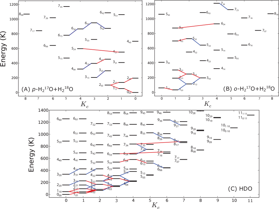
Figure 1: Observed transitions of H₂¹⁸O, H₂¹⁷O, and HDO with HIFI. The lines indicate detected transitions; heavily blended lines (i.e. those judged to be too blended to extract reliable fit Gaussian parameters) are omitted. Red lines indicate transitions in bands 1-5 of HIFI, while blue lines indicate transitions in bands 6 and 7. For panels A and B, a transition is indicated if it is clearly detected in either H₂¹⁸O or H₂¹⁷O; for some transitions, due to blends or intensity, both isotopologues are not used in the analysis.

As in previous high-spectral resolution surveys of Orion KL, many molecular transitions exhibit complex lineshapes, corresponding to contributions from multiple spatial components known to exist in this source within the Herschel beam. Physical and kinematic properties of the three canonical spatial components can be found in Table 1, and are discussed briefly below:

• Hot Core: This region has a complex structure, with a number of radio and infrared continuum sources (Genzel & Stutzki, 1989; Menten & Reid, 1995; Beuther et al., 2004). It has been proposed that the Hot Core region is heated by the remnants of a recent explosive event (Zapata et al., 2011; Bally et al., 2011; Nissen et al., 2012) rather than active star formation.

• Compact Ridge: This is also a structurally complex region, particularly in the observed molecular emission morphologies (Friedel & Snyder, 2008; Guélin et al., 2008; Favre et al., 2011; Neill et al., 2011; Brouillet et al., 2013), and has also been suggested to have been heated externally (Blake et al., 1987; Wang et al., 2011).

• Plateau: There are two prominent ouflows centered in the Orion KL region (Genzel et al., 1981; Genzel & Stutzki, 1989; Greenhill et al., 1998). The so-called High-Velocity Flow is oriented in the SE–NW direction and characterized by velocities of up to 150 km s^-1, while the Low-Velocity Flow ($\Delta v\sim 18$ km s^-1) is oriented in the NE–SW direction. In some transitions of water, the blue-shifted wing of the outflow component is found to be in absorption against the strong far-infrared dust continuum (Cernicharo et al., 2006).

Table 1: Kinematic parameters and physical conditions of the Orion KL spatial components.

Component	$\theta_{s}$	$v_{\textnormal{LSR}}$	$\Delta v$	$T_{\textnormal{kin}}$	$n$(H2)	$N$(H2)
	$(^{\prime\prime})$	(km s-1)	(km s-1)	(K)	(cm${}^{-3})$	(cm${}^{-2})$
Hot Core	5–10	3–5	5–10	150–300	$10^{7}$–$10^{8}$	$3.1\times 10^{23}$
Compact Ridge	5–15	7–9	3–5	80–125	$10^{6}$–$10^{7}$	$3.9\times 10^{23}$
Plateau	20–30	6–12	20–25	100–150	$10^{6}$–$10^{7}$	$1.8\times 10^{23}$

The Orion KL region also has an extended ridge, which consists of cooler ($\sim 60$ K) and less dense ($n$(H₂) $\sim 10^{5}$ cm^-3) quiescent gas extended across the Herschel beam. This component has very similar kinematic properties to the Compact Ridge ($v_{\textnormal{LSR}}=9$ km s^-1, $\Delta v=4$ km s^-1, Blake et al. (1987)), and may contribute some flux to the lowest-energy lines, which would most likely be incorporated into the Compact Ridge spectral component. We expect this contribution to be minor, because H₂O transitions are likely very subthermally excited at the physical conditions of the extended ridge.

Each transition was fit with up to four Gaussian components using CLASS, depending on which of the spatial components were detected. Some low-energy transitions, as in previous measurements, are found to have absorption in the blue-shifted wing; the modeling of these transitions is described in more detail in §3.5. For many of the transitions, particularly the lowest-energy transitions which have contributions from all three spatial components, it was found to be necessary to constrain some of the line positions and widths in order to reduce the number of free parameters. Where this was needed, the values in Table 1 were used. For HD¹⁸O and D₂O, the line profiles were well fit by single Gaussian components. The parameters of the Gaussian fits for all isotopologues can be found in the Appendix (Tables 3-6).

3.2 Strategy for column density derivations

Here the approaches used to derive the H₂O and HDO abundances in the different spatial/velocity components within Orion KL are described. Even for the minor isotopologues analyzed here, many transitions are not optically thin. For H₂¹⁸O and H₂¹⁷O, the optical depth can be determined by comparing transitions of the two isotopologues, using the following equation:

$$\frac{\Delta T_{\textnormal{mb}}(\textnormal{H}_{2}\,\!^{18}\textnormal{O})}{\Delta T_{\textnormal{mb}}(\textnormal{H}_{2}\,\!^{17}\textnormal{O})}=\frac{J(T_{\textnormal{ex},18})(1-e^{-\tau_{18}})}{J(T_{\textnormal{ex},17})(1-e^{-\tau_{17}})}=\frac{(1-e^{-\tau_{18}})}{(1-e^{-\tau_{17}})}$$ (1)

where we assume the same excitation temperature between transitions with the same quantum numbers of H₂¹⁸O and H₂¹⁷O; therefore, $\tau_{18}/\tau_{17}$ is the H₂¹⁸O/H₂¹⁷O abundance ratio. We assume ¹⁶O/¹⁸O = $250\pm 135$ (Tercero et al., 2010) and ¹⁸O/¹⁷O = $3.6\pm 0.7$ (Persson et al., 2007). This ¹⁶O/¹⁸O ratio was derived by Tercero et al. (2010) from a comparison of ¹⁶OCS and ¹⁸OCS in the Plateau; in the Hot Core and Compact Ridge only lower limits could be estimated for the ¹⁶O/¹⁸O ratio because of optical depth. Tercero et al. (2010) do note that optical depth in the normal isotopologue could still be an issue for the Plateau, so their observations may be consistent with the solar value of 500. A recent analysis of C¹⁸O and C¹⁷O in the Orion KL HIFI spectrum by Plume et al. (2012) suggested different ¹⁸O/¹⁷O isotopic ratios between spatial components: they derived a ratio of $3.0_{-1.1}^{+1.2}$ for the Hot Core and $4.1_{-1.3}^{+2.1}$ for the Compact Ridge, within the $1\sigma$ errors of the ratio adopted here ($3.6\pm 0.7$). In the Plateau, Plume et al. (2012) derive a C¹⁸O/C¹⁷O ratio of $1.7_{-0.5}^{+0.4}$, which they suggest could be due to isotopically selective photochemistry. Here, however, we assume the same oxygen isotopic ratios for all spatial components.

Figure 2 shows the comparison of three corresponding transitions of H₂¹⁸O and H₂¹⁷O. In the first row, where a transition with $E_{\textnormal{up}}=136$ K is shown, it can be seen that much of the flux for low-energy transitions is in the broad Plateau component, but the narrower Hot Core and Compact Ridge components are also clearly visible. For all three components, a visual inspection reveals that the H₂¹⁸O/H₂¹⁷O flux ratio is significantly less than the assumed abundance ratio of 3.6, indicative of significant optical depth. For the Hot Core, the flux is greater in the H₂¹⁷O transition than in H₂¹⁸O. This is observed in several lines with $E_{\textnormal{up}}<400$ K; this is likely due to foreground extinction of Hot Core emission by the outflow, which is moderately optically thick in H₂¹⁸O; this was previously suggested by Pardo et al. (2001). For the second row in Figure 2, where a transition with $E_{\textnormal{up}}\sim 450$ K is shown, emission from only the Plateau and Hot Core components is detected. In the bottom row, where a high-excitation line ($E_{\textnormal{up}}=728$ K) is shown, the transitions are well-modeled with a single Gaussian component, attributed to the Hot Core. In Figure 3, a sample of HDO lines are presented, while in Figure 4 we show the detected lines of HD¹⁸O and D₂O.

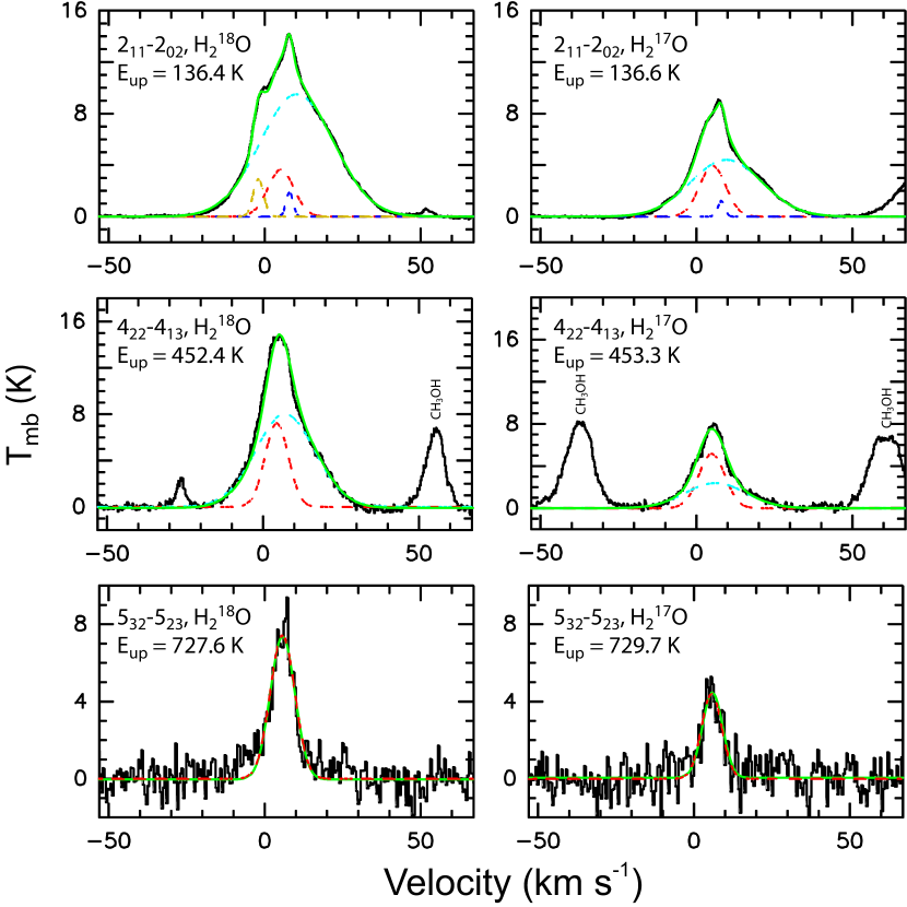
Figure 2: Gaussian fits to lines of H₂¹⁸O and H₂¹⁷O. In each panel, the green curve is the total fit to the data, while the cyan, red, and blue curves indicate the Gaussian components attributed to the outflow, Hot Core, and Compact Ridge, respectively. In the top-left panel, the yellow curve is the $10_{10,*}-9_{9,*}$ multiplet of CH₃OCH₃ from the HIFI fullband model. The spectra (in black) in this figure are continuum-subtracted.

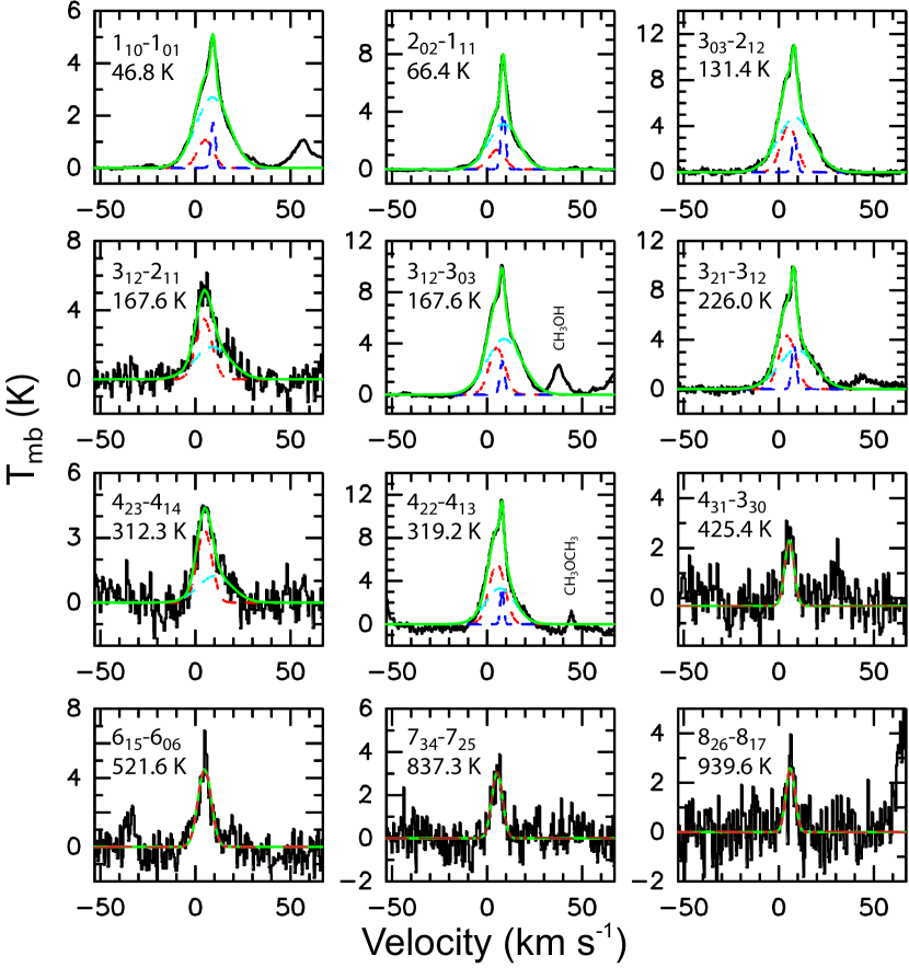
Figure 3: Gaussian fits to a selection of HDO transitions detected by HIFI. In each panel, the green curve is the total fit to the data, while the cyan, red, and blue curves indicate the Gaussian components attributed to the outflow, Hot Core, and Compact Ridge spatial components, respectively. The quantum numbers and the upper-state energy of each transition are specified. The spectra (in black) in this figure are continuum-subtracted.

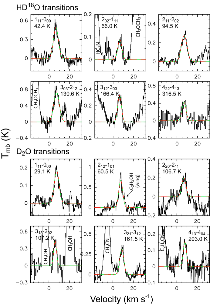
Figure 4: Detected transitions of HD¹⁸O and D₂O. The red curves indicate single-Gaussian fits to the data. The quantum numbers and upper-state energy are indicated for each transition. The spectra (in black) in this figure are continuum-subtracted.

Because the H₂ density within Orion KL is likely lower than is required to collisionally thermalize all of the observed transitions, the level populations are expected to deviate significantly from local thermodynamic equilibrium (LTE). Additionally, the excitation of water is strongly influenced by the local far-infrared radiation field (Jacq et al., 1990; Cernicharo et al., 2006; Melnick et al., 2010; van Dishoeck et al., 2011). We have therefore included a background continuum field based on far-infrared observations of Orion KL, which is presented in Figure 5. Further information on this continuum can be found in Crockett et al. (2013a, in preparation). The observations derive from the continuum level measured by HIFI in the Orion KL fullband survey for $\lambda=$ 600–160 $\upmu$m, and from Infrared Space Observatory surveys for shorter wavelengths (van Dishoeck et al., 1998; Lerate et al., 2006). The ISO observations are scaled to match those from HIFI at their intersection wavelength ($160$ $\upmu$m). Because the HIFI beam at this wavelength ($11^{\prime\prime}$) is smaller than that of ISO-LWS ($\sim$80^′′), the higher continuum flux measured by HIFI is attributed to greater beam dilution in ISO. The resulting continuum (in black in Figure 5) is referred to here as the “observed continuum.”

A recent study of the excitation of H₂S in the Orion Hot Core with the HIFI fullband survey (Crockett et al. 2013a, in prepration) has found that reproducing the observed line fluxes, particularly for the highest energy levels, requires an enhancement of a factor of 8 for $\lambda<100$ $\upmu$m above the observed continuum in Figure 5, a possible indication of hidden luminosity from hot dust in the Hot Core not directly detectable due to high optical depth but important in the excitation of hydride molecules with transitions in the far-infrared. The Hot Core has been previously suggested to have high optical depth in the far-IR on the basis of modeling of high-excitation NH₃ (Hermsen et al., 1988) and HDO (Jacq et al., 1990) transitions. As will be discussed further in §3.3 below, better agreement is found with the observed line fluxes of H₂O and HDO in the Hot Core when the continuum is enhanced by a factor of 3 in the far-IR. This continuum is plotted in green in Figure 5 and referred to as the “enhanced continuum” in this work. For $\lambda>100$ $\upmu$m, the dust optical depth is lower, so it is less likely that the true continuum field seen by the molecular gas is significantly enhanced over the observed continuum. The H₂O and HDO excitation is less sensitive to radiative pumping at longer wavelengths, so this makes little impact on the derived abundances. For the Compact Ridge and Plateau spatial components, far-infrared excitation is also important, and for these components the observed continuum in Figure 5 is used.

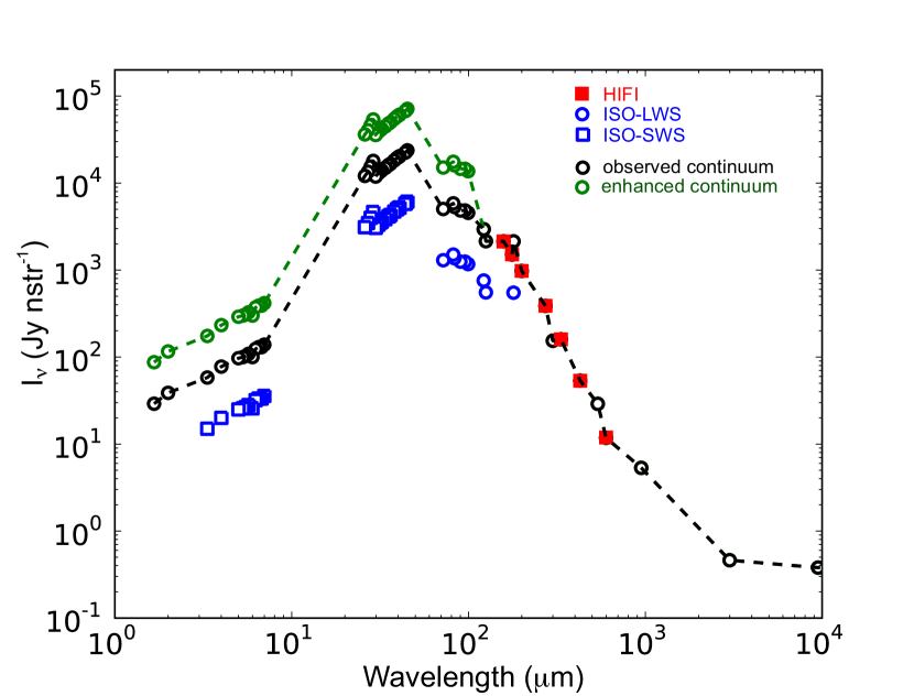
Figure 5: Orion KL continuum radiation field used for modeling of H₂O and HDO emission. The blue and red points indicate measurements, as indicated. The ISO-LWS measurements are from Lerate et al. (2006); ISO-SWS measurements are from van Dishoeck et al. (1998); and the HIFI measurements are from the Orion KL fullband survey (Bergin et al., 2010). The black and green curves show the “observed” and “enhanced” continuum fields used in RADEX modeling. See the text and Crockett et al. (2013a, in preparation) for further information.

We have used two different approaches to derive the column densities of H₂O and HDO; the method used for a given spatial component depends on the reliability of the optical depth estimates for each component and the number of transitions observed to emit from the component. The first approach is to directly sum the populations of each observed level (Goldsmith et al., 1997; Plume et al., 2012). Figure 1 shows that particularly for low-lying ($E<400$ K) energy levels where most of the population is found, transitions are detected originating from most levels. From each transition, the population in the upper state can be derived using (Goldsmith & Langer, 1999)

$$N_{u}=\frac{1.67\times 10^{17}Wg_{u}}{\nu S_{\textnormal{ij}}\mu^{2}\eta_{\textnormal{bf}}}\frac{\tau_{l}}{1-\textnormal{e}^{-\tau_{l}}}$$ (2)

where $N_{u}$ is the upper state column density in cm^-2, $W$ is the integrated flux in K km s^-1, $g_{u}$ is the upper state degeneracy, $\nu$ is the frequency in MHz, $S_{\textnormal{ij}}\mu^{2}$ the line strength in debye², $\eta_{\textnormal{bf}}$ the beam dilution factor, and $\tau_{l}$ the line optical depth. The column densities in individual levels derived by equation (2) are independent of the excitation mechanism, whether through collisions or radiative excitation. In order to derive a total column density, the following equation is used:

$$N_{\textnormal{total}}=f_{c}\sum N_{\textnormal{observed}}$$ (3)

In this equation, $f_{c}$ is a correction factor to account for the population that is located in levels that cannot be derived by equation (2). These factors are calculated from 1-D large velocity gradient calculations using the publicly available RADEX code (van der Tak et al., 2007). The physical parameters from Table 1 are used for these calculations. Where this approach, referred to here as the population summation method, is not possible, we have used the RADEX code to derive the column density and physical parameters that best reproduce the observed measurements, which will be described in more detail in the sections to follow.

These models use collisional rates for isotopologues of water with H₂ from the LAMDA database (Schöier et al., 2005). For H₂¹⁸O and H₂¹⁷O, the rates from Daniel et al. (2011) for collisions of H₂O with H₂ are used, while for HD¹⁶O and HD¹⁸O we use the rates of Faure et al. (2012) for HDO. For all isotopologues, the rates were calculated for collisions with both o-H₂ and p-H₂, and a thermal ortho/para H₂ ratio is assumed in all models. While transitions of HDO with energies up to 1200 K are detected, the available collision rates for HDO only include energy levels up to $E=450$ K. At the present time, therefore, we cannot model the highest-energy transitions of HDO detected by HIFI. Additionally, the models presented here do not include the effect of radiative pumping through vibration-rotation transitions. If this excitation pathway is important, it could change the physical parameters derived in this study. However, for each component enough transitions are detected that the abundance is well constrained, despite uncertainty in the precise excitation mechanism.

In the following subsections, we discuss in detail the derivation of the H₂O and HDO column densities in each component, which are summarized in Table 2. In this table we present the column density of HDO relative to both H₂¹⁸O and H₂¹⁶O. For most components, the HDO/H₂O ratio is dependent on the ¹⁶O/¹⁸O ratio. The uncertainty in this ratio is therefore a major contributor to the uncertainty in the absolute HDO/H₂O ratio for each component, so for comparison of the deuterium fractionation between the different components within Orion KL, the [HD¹⁶O]/[H₂¹⁸O] ratio is more representative of the relative uncertainties.

Table 2: Summary of H₂O and HDO column densities in Orion KL.

Component	$\theta_{s}$	$N$(H218O)	$\chi$(H2O)	$N$(HDO)	[HD16O]/[H218O]	[HDO]/[H2O]
	$(^{\prime\prime})$	(cm-2)		(cm-2)
Hot Core (7 km s-1)	2	$8.0_{-4.0}^{+8.0}\times 10^{17}$	$6.5_{-4.8}^{+7.3}\times 10^{-4}$	$6.0_{-3.6}^{+3.6}\times 10^{17}$	$0.75_{-0.58}^{+0.88}$	$3.0_{-1.7}^{+3.1}\times 10^{-3}$
Hot Core (5 km s-1)	5	$\geq 9.0\times 10^{15}$	$\geq 7.3\times 10^{-6}$	$\geq 6.2\times 10^{15}$	0.69	$2.8\times 10^{-3}$
Compact Ridge	6	$4.1_{-0.9}^{+1.0}\times 10^{15}$	$2.6_{-1.5}^{+1.6}\times 10^{-6}$	$3.9_{-1.2}^{+2.9}\times 10^{15}$	$0.95_{-0.36}^{+0.74}$	$3.8_{-2.5}^{+3.6}\times 10^{-3}$
Plateau (emission)	30	$3.5_{-0.6}^{+0.6}\times 10^{15}$	$4.8_{-2.8}^{+2.8}\times 10^{-6}$	$1.23_{-0.25}^{+0.25}\times 10^{15}$	$0.35_{-0.09}^{+0.09}$	$1.4_{-0.8}^{+0.8}\times 10^{-3}$
Absorbing gas	$\theta_{b}$	$9.8_{-2.9}^{+4.0}\times 10^{14}$	$2.7_{-1.6}^{+1.6}\times 10^{-6}$	$5.5_{-0.7}^{+0.6}\times 10^{13}$	$0.056_{-0.013}^{+0.014}$	$2.2_{-1.3}^{+1.3}\times 10^{-4}$

3.3 Hot Core

3.3.1 HDO and HD¹⁸O

The detection of HD¹⁸O toward Orion KL was first reported by Bergin et al. (2010), to date the only time this species has been identified in the interstellar medium. This detection implies a region with a very high HDO column density within the Herschel beam. HDO emission from the component that is emissive in HD¹⁸O must have very high optical depth in the corresponding HD¹⁶O transitions (comparing Figures 3 and 4). The HD¹⁸O lines have an average $v_{\textnormal{LSR}}=6.7$ km s^-1 and $\Delta v=5.4$ km s^-1, both of which are intermediate between the canonical parameters for the Compact Ridge and Hot Core given in Table 1. This detection was initially reported as tenative by Bergin et al. (2010). The fullband model to the HIFI spectrum (Crockett et al. 2013b, in preparation) does not have any substantial ($>0.1$ K) transitions of other species coincident in frequency with any of these six transitions. An LTE model to the six transitions of HD¹⁸O does not predict any lines to be emissive that are missing; due to the high line density of the Orion KL spectrum, there are several potentially emissive transitions that lie under strong lines of other species. We conclude that the assignment of these six transitions to HD¹⁸O is correct. The high HDO column density implied by this detection requires one of two explanations: either the HD¹⁸O-emitting component has a high [HDO]/[H₂O] ratio as compared to the “normal” D/H ratios previously found for water and other species in Orion KL ($\sim 10^{-3}$–$10^{-2}$), or this component also has a high H₂O abundance. The $2_{20}-2_{21}$ transition of HDO at 10.3 GHz was detected by Petuchowski & Bennett (1988) with similar kinetic parameters as the HD¹⁸O transitions. This detection was surprising considering the low Einstein A coefficent of this transition ($3.6\times 10^{-9}$ s^-1) and was interpreted as evidence of a high HDO abundance in a highly excited clump of gas.

In order to determine the spatial origin of the HD¹⁸O emission, we use two transitions of HDO that were detected in the Orion KL ALMA survey: the $3_{12}-2_{21}$ transition at 225896.7 MHz ($E_{\textnormal{up}}=167.6$ K, $S_{\textnormal{ij}}\mu^{2}=0.69$ D²) and the $2_{11}-2_{12}$ transition at 241561.6 MHz ($E_{\textnormal{up}}=95.2$ K, $S_{\textnormal{ij}}\mu^{2}=0.36$ D²). There is also a third potentially detectable transition of HDO in the dataset (the $7_{34}-6_{43}$ transition at 241.973 GHz), but this line is blended with a strong transition of C₂H₅CN. Figure 6 shows images of these two transitions, integrated over $\sim 2.5$ km s^-1 velocity widths. Both of these transitions appear to be free of significant emission from other molecules, and the emission morphologies of the two transitions are very similar. The 225 GHz transition was found in LVG modeling by Faure et al. (2012) to exhibit a moderate population inversion ($|\tau|\leq 1$) under high densities and temperatures like the conditions within Orion KL, but the 241 GHz transition did not. In the first row, in the velocity range of 2.8–5.7 km s^-1, the strongest emission comes from the Hot Core region, near the region of strongest 230 GHz continuum emission, with a second component near the IRc7 infrared continuum source. In the second row, it can be seen that the strongest emission in the 6.3–8.9 km s^-1 velocity range is located about $1^{\prime\prime}$ south of the dust continuum peak, centered at $\alpha_{\textnormal{J2000}}$ = 05${}^{\textnormal{h}}$35${}^{\textnormal{m}}$14${}^{\textnormal{s}}$.54, $\delta_{\textnormal{J2000}}$ = -05${}^{\circ}22^{\prime}33^{\prime\prime}$. This spatial component peaks at a velocity of 7 km s^-1, in agreement with the velocity of the HD¹⁸O lines in HIFI. Lastly, in the third row, showing velocities between 9.5–11.5 km s^-1, in addition to the Hot Core emission (which is the red wing of the 7 km s^-1 component), emission from the Compact Ridge (to the southwest of the Hot Core) and a clump to the northwest can be seen. The emission in this velocity range is weaker than in the other two rows; note that the color scale is more sensitive by a factor of $\sim 3$ in the third row. The ALMA observation was performed without zero-spacing information. Therefore, to judge the degree to which these observations may be missing extended emission, we compared the line fluxes to the single-dish observations of these two transitions with the IRAM 30 m telescope by Jacq et al. (1990). The ALMA images were smoothed to a spatial resolution of $10.5^{\prime\prime}$, the beamwidth at the 30 m telescope at this frequency, and found that 80–90% of the flux of these two transitions is recovered by ALMA.

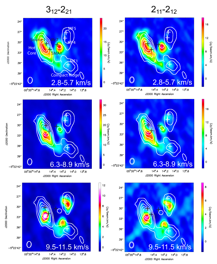
Figure 6: Emission of two transitions of HDO toward Orion KL as measured by ALMA. In each panel, the integrated HDO emission over the given velocity range is in color scale, while the white contours (levels (0.1, 0.2, 0.4, 0.6, 0.8) $\times$ 1.34 Jy beam^-1) indicate the continuum emission level. The black crosses indicate three of the continuum sources in this region: (from left to right) source I, SMA1, and IRc7. The white crosses indicate peaks in methyl formate emission in the nomenclature of Favre et al. (2011). The ovals in the lower left corner of each panel indicate the synthesized beam.

The agreement between the velocity of the region with strongest HDO emission in Orion KL in the ALMA images in Figure 6 and the velocity of the detected HD¹⁸O lines by HIFI allows us to assign the HD¹⁸O emission to the clump to the south of the Hot Core region. Motivated by these maps, we model the water emission in the Hot Core with two spatial/velocity components, one for the 7 km s^-1 clump and a second centered at the canonical Hot Core velocity of 5 km s^-1, consisting of the emission components in the top row of Figure 6. We assume that all of the HD¹⁸O emission comes from the 7 km s^-1 component, and we begin with models to derive the HDO abundance in this component. In Figure 7, two single-component models of the Hot Core emission of HDO and HD¹⁸O are shown. The points indicate the fluxes for each transition; for HD¹⁶O, because the Hot Core is fit as a single Gaussian component, it represents the total flux summed over the two components. These models are calculated with a kinetic temperature of 200 K, an H₂ density of 10⁸ cm^-3, and the enhanced background continuum field shown in Figure 5. If the observed continuum is used instead, an equally good fit can be obtained with a higher H₂ density ($10^{9}$ cm^-3), which may be reasonable over a small region. As discussed in §3.3.2 below, the high-energy ($E_{u}>500$ K) H₂O lines are best modeled with the enhanced continuum, so for consistency, we also use the enhanced field for the models in Figure 7. The derived HDO column density is insensitive to these two excitation scenarios.

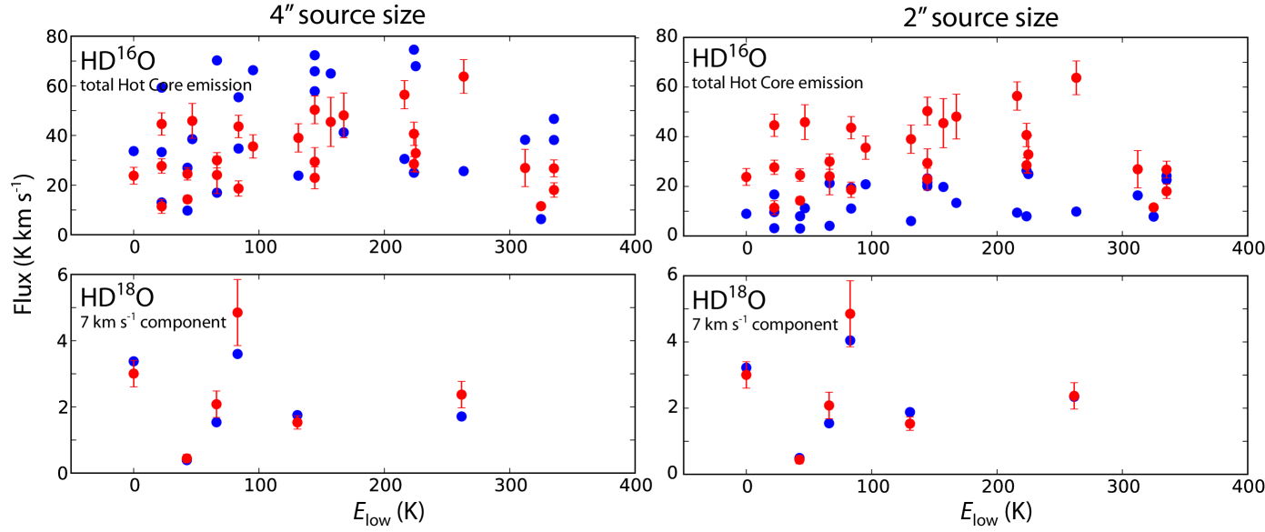
Figure 7: RADEX models of HDO and HD¹⁸O to the 7 km s^-1 component in the Hot Core. In all panels, the red circles (with error bars) represent the observed line fluxes as a function of lower-state energy, while the blue circles are the integrated line fluxes calculated by the models. The left column is with a source size of $4^{\prime\prime}$ and $N$(HD¹⁸O) = $4.0\times 10^{14}$ cm^-2, while the model in the right column has a source size of $2^{\prime\prime}$ and $N$(HD¹⁸O) = $2.4\times 10^{15}$ cm^-2. An HD¹⁶O/HD¹⁸O ratio of 250 is assumed. Both models use $T_{\textnormal{kin}}$ = 200 K, $n$(H₂) = $10^{8}$ cm^-3, and the enhanced far-infrared radiation field as described in the text.

The two models in Figure 7 differ in the size of the emitting region. For a source size of $4^{\prime\prime}$ (left column), the fluxes of the HD¹⁸O lines are well reproduced, but many of the lines of HD¹⁶O are overpredicted, some by as much as a factor of 3. While the outflow component of the HDO transitions could have significant optical depth in some lines and therefore could hide the Hot Core component in some of these lines (Pardo et al., 2001), it is unlikely that the extinction is this significant in all of these transitions, particularly as the Plateau component is weak in the higher-energy lines. Therefore, the most likely explanation is that the emitting region responsible for the HD¹⁸O lines is smaller than $4^{\prime\prime}$, and the HDO emission from the same region is more optically thick. The right panel shows that with a source size of $2^{\prime\prime}$ and a column density $N$(HD¹⁸O) = $2.4\times 10^{15}$ cm^-2, and the same excitation parameters otherwise, the HD¹⁸O lines are still well modeled, but the optical depth in the HD¹⁶O transitions is high enough to keep the these lines from being overpredicted. A source size of $2^{\prime\prime}$ also agrees well with the size of the bright 7 km s^-1 clump in the HDO ALMA images in Figure 6. Therefore, we adopt $2^{\prime\prime}$ as the size of the HD¹⁸O emitting region, and $(2.4\pm 0.6)\times 10^{15}$ cm^-2 as the HD¹⁸O column density. This 25% uncertainty is attributed primarily to the uncertainty in the excitation of the HD¹⁸O transitions. This leads to an HDO column density of $(6.0\pm 3.6)\times 10^{17}$ cm^-2.

In the HD¹⁶O panel of the $2^{\prime\prime}$ model in Figure 7, the difference between the observed fluxes and the calculated fluxes of the 7 km s^-1 component is attributed to the second Hot Core component (centered at 5 km s^-1). We adopt a source size of $5^{\prime\prime}$ for this component, and use the population summation method described in §3.2. We subtract from the observed flux of each line the flux predicted by the $2^{\prime\prime}$ model to the 7 km s^-1 component in Figure 7, and then apply equation (1) to derive an upper state column density for each transition, assuming that the emission from this component is optically thin. There are several cases where two transitions with the same upper state are observed; these line pairs suggest that some transitions in this component have moderate optical depth. For these cases, we use the transition with lower optical depth to estimate the population in that level. However, as we do not have information about the optical depth for most levels of HDO, this column density should be viewed as a lower limit. We calculate a correction factor of 1.42, which is derived as described above using RADEX, assuming $T_{\textnormal{kin}}=200$ K, $n$(H₂) = $10^{8}$ cm^-2, and using the enhanced continuum field. With this, an HDO column density of $6.2\times 10^{15}$ cm^-2 for the 5 km s^-1 Hot Core component is derived.

3.3.2 H₂¹⁸O and H₂¹⁷O

The analysis of H₂O in the Hot Core is complicated by the fact that a comparison of H₂¹⁸O and H₂¹⁷O, as described above, shows that many of the lower-energy transitions are very optically thick, so they contain little to no information on the column density in those levels; also, as noted above, the Plateau could be attenuating the Hot Core emission in some lines. The only transitions of H₂¹⁸O or H₂¹⁷O that might be optically thin are the high-energy lines, so we first turn our attention to the highest-energy transitions before returning to discuss the lower-energy, optically thick lines. The high-energy transitions (here defined as $E_{\textnormal{up}}>500$ K) that fall in the HIFI bandwidth can be broadly segregated into two sets based on their line strengths: $\Delta J$ = 0 transitions, which have high line strengths ($S_{\textnormal{ij}}\mu^{2}>10$ D²), and $\Delta J$ = 1 transitions, which are are considerably weaker ($S_{\textnormal{ij}}\mu^{2}<3$ D²). These transitions therefore span a wide range in optical depth. As with the HD¹⁸O transitions, the detection of these low-$S_{\textnormal{ij}}\mu^{2}$, high-energy H₂¹⁸O transitions indicate a component with a high H₂O abundance.

Figure 8 shows transitions of H₂¹⁸O and H₂¹⁷O with $E_{\textnormal{up}}>500$ K. Several of the lines, particularly the lines of H₂¹⁷O, are only marginally detected, and three are blended with lines of CH₃OH. The two overlaid models have source sizes of $4^{\prime\prime}$ (dashed red lines) and $2^{\prime\prime}$ (solid red lines). Both models have $T_{\textnormal{kin}}=200$ K and $n$(H₂) = $10^{8}$ cm^-3, and the enhanced continuum field from Figure 5. For both models, the low-$S_{\textnormal{ij}}\mu^{2}$ transitions are well reproduced, with the exception of the $6_{33}-5_{42}$ transition; this line is not well reproduced with any model that does not overpredict other transitions substantially, so this line may be blended with an unidentified transition from another molecule. However, for the $4^{\prime\prime}$ source size model, with the column density required to reproduce the flux of the low-$S_{\textnormal{ij}}\mu^{2}$ transitions, the high-$S_{\textnormal{ij}}\mu^{2}$ transitions are overpredicted. The $2^{\prime\prime}$ model, alternatively, is in better agreement. This model has a H₂¹⁸O column density of $8.0\times 10^{17}$ cm^-2, which implies a H₂¹⁶O column density of $2.0\times 10^{20}$ cm^-2. We assume a factor of 2 uncertainty in the H₂¹⁸O column density: in the models presented in Figure 8, $\sim$90% of the population is located in states with $E_{\textnormal{up}}<$ 500 K, but, due to high optical depth, there is little to no direct sensitivity to the population in these levels. Using an H₂ column density of $3.1\times 10^{23}$ cm^-2 (Plume et al., 2012), this corresponds to an H₂O abundance relative to H₂ of $6.5_{-4.8}^{+7.3}\times 10^{-4}$, making H₂O the predominant form of oxygen: the H₂O column density we derive relative to H ($\approx 2N$(H₂)) is $3.25\times 10^{-4}$, while the Orion Nebula has been found to have total [O]/[H] $\sim 4\times 10^{-4}$ (Wilson & Rood, 1994; Rubin et al., 1991; Baldwin et al., 1991). It should be noted, however, that the value used for the H₂ column density was derived for the Hot Core as a whole, and may be higher in the localized $2^{\prime\prime}$ region under consideration. Interferometric studies deriving H₂ column densities from millimeter dust emission have found $N$(H₂) $\geq 10^{24}$ cm^-2 over small spatial scales in the center of the Hot Core region (Blake et al., 1996; Beuther et al., 2004; Favre et al., 2011).

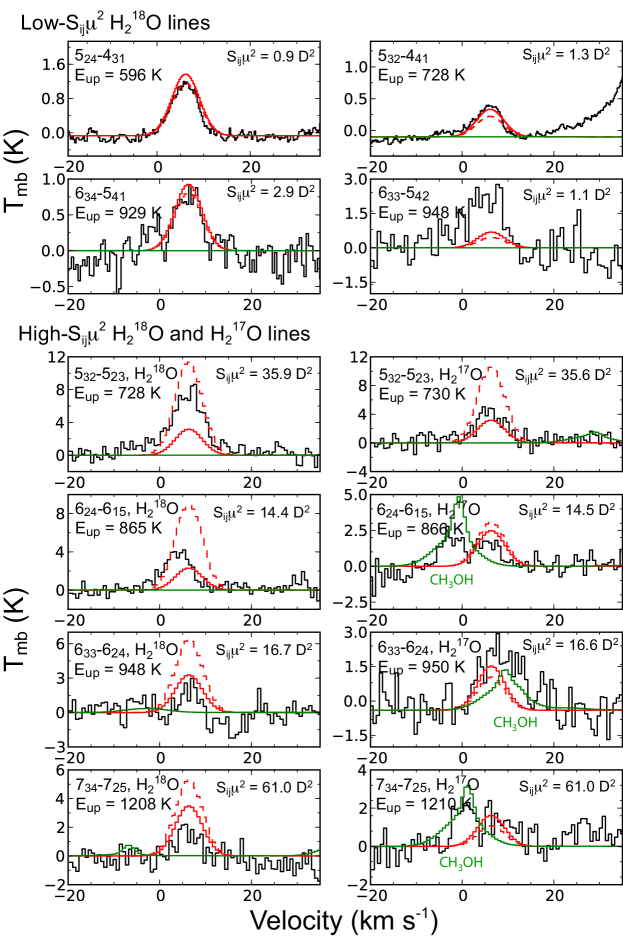
Figure 8: High-excitation ($E_{\textnormal{up}}>500$ K) transitions of H₂¹⁸O and H₂¹⁷O detected (or tentatively detected) toward the Hot Core. In each panel, the black curves are the data (smoothed to $\sim 1.5$ km s^-1 to reduce the noise level); the dashed red lines are a RADEX model with $\theta_{s}=4^{\prime\prime}$ and $N$(H₂¹⁸O) = $2.0\times 10^{17}$ cm^-2; and the solid red lines are a RADEX model with $\theta_{s}=2^{\prime\prime}$ and $N$(H₂¹⁸O) = $8.0\times 10^{17}$ cm^-2; and the green lines are the HIFI fullband model (Crockett et al. 2013b, in preparation). The assumed kinematic parameters for the synthetic line profiles are $v_{\textnormal{LSR}}=6.0$ km s^-1 and $\Delta v=7.0$ km s^-1. Both models have $T_{\textnormal{kin}}=200$ K, $n$(H₂) = $10^{8}$ cm^-3, and an enhanced far-IR radiation field as described in the text.

In the models in Figure 8, we assume a ortho:para ratio of 3 for the H₂O isotopologues. We examined the effect of the ortho:para ratio on our H₂O models by instead assuming a ratio of 1.5 and re-running the models in Figure 8: we find that the fit is slightly worse (particularly on the low-$S_{\textnormal{ij}}\mu^{2}$ lines), but only marginally, so these models are formally consistent with either ortho:para ratio. The adopted ortho:para ratio does not make a dramatic difference in the total H₂O column density. We also assume that the highly excited $2^{\prime\prime}$ H₂O component is cospatial with the $2^{\prime\prime}$ HDO component from which HD¹⁸O emission is detected. In the models shown in Figure 8, kinematic parameters of $v_{\textnormal{LSR}}=6.0$ km s^-1 and $\Delta v=7.0$ km s^-1 are assumed for the plotted Gaussians, close to the parameters of the HD¹⁸O transitions. It can be seen that the line profiles are generally in good agreement with the observations. The analyses of HDO and H₂O above indicate that both molecules arise in a small clump with high abundance in the Orion Hot Core region, as evidenced by the detection of weak transitions (the rare HD¹⁸O isotopologue, and the low-$S_{\textnormal{ij}}\mu^{2}$ transitions of H₂¹⁸O). Therefore, the most likely explanation is that they are cospatial.

Just as for HDO, this $2^{\prime\prime}$ component does not explain all of the flux for the lower-energy H₂¹⁸O and H₂¹⁷O transitions. As in §3.3.1, we assume that the remainder of the flux is attributed to the rest of the Hot Core region (the 5 km s^-1 component), for which a source size of $5^{\prime\prime}$ is assumed. To derive the column density of this component, we use the H₂¹⁷O transitions, subtract the flux predicted by the model to the $2^{\prime\prime}$ component described above, and derive the upper state column densities for each transition, assuming that the second component is optically thin. As this may not be true, this column density should be viewed as a lower limit. Assuming $T_{\textnormal{kin}}=200$ K and $n$(H₂) = $10^{8}$ cm^-3, a correction factor of 2.1 is calculated for ortho-H₂¹⁷O, and 2.3 for para-H₂¹⁷O, which yields a H₂¹⁷O column density of $2.5\times 10^{15}$ cm^-2. This implies a H₂¹⁶O column density of $2.3\times 10^{18}$ cm^-2.

3.3.3 D₂O

The D₂O isotopologue was first identified in the interstellar medium in IRAS 16293-2422 (Butner et al., 2007; Vastel et al., 2010). Six transitions of D₂O were detected in Orion KL in the HIFI survey, with an average $v_{\textnormal{LSR}}=7.5$ km s^-1 and $\Delta v=4.3$ km s^-1. As with the HD¹⁸O lines, these are anticipated to be the most emissive transitions of D₂O in the HIFI bandwidth (neglecting lines that are not detected due to blends with stronger transitions of other molecules). The kinematic parameters of the D₂O transitions are slightly different from those for HD¹⁸O or the high-energy H₂¹⁸O transitions, but the differences are small enough that we consider the most likely possibility to be that these components are mostly cospatial. Collisional excitation rates for D₂O were recently published (Faure et al., 2012) but extend up to only $T_{\textnormal{kin}}=100$ K and are available only for low-lying energy levels, so instead we model this molecule with a LTE rotation diagram analysis (Goldsmith & Langer, 1999), assuming a statistical ortho:para ratio of 2:1 (different from the 3:1 of H₂O because of the difference between hydrogen and deuterium spin statistics). Assuming all lines are optically thin, a rotational temperature of $74\pm 27$ K is derived. A similar analysis of the six detected transitions of HD¹⁸O yields a rotational temperature of $T_{\textnormal{rot}}=104\pm 14$ K, in statistical agreement with the temperature derived for D₂O. Assuming the same $2^{\prime\prime}$ source size as for the high-abundance ($v_{\textnormal{LSR}}\sim 7$ km s^-1) H₂O and HDO component, we derive $N$(D₂O) = $(9.6\pm 5.5)\times 10^{14}$ cm^-2. This results in a value of [D₂O]/[HDO] = $0.0016\pm 0.0013$ in this component.

3.4 Compact ridge

The Compact Ridge component, as Figures 2 and 3 show, appears as a narrow spike in the line profile. As indicated in Table 1, the Compact Ridge has generally been found to be cooler and less dense than the Hot Core (Blake et al., 1987; Tercero et al., 2010). Figure 6 shows that HDO emission in the 8–11 km s^-1 velocity range arises from both the Compact Ridge region and a clump to the northwest (MF4/MF5 in the nomenclature of Favre et al. (2011)). However, for this analysis we treat this spectral component as a single homogeneous one with a diameter of $6^{\prime\prime}$, based on the spatial extent of the HDO emission in the Compact Ridge velocity range in the ALMA images. This component appears only in the lower-energy lines ($E_{\textnormal{up}}<310$ K), indicating that the molecular gas in the Compact Ridge is less excited than in the Hot Core. Additionally, this component is not detected in most of the lines in bands 6–7 (where the noise level is highest). Therefore, particularly for H₂O, the population summation method cannot be used reliably: combining H₂¹⁸O and H₂¹⁷O, the 10 transitions with a detected Compact Ridge component (5 for each isotopologue) include only 6 upper-state energy levels, 3 of ortho and 3 of para. For HDO, a total of 14 transitions have detected Compact Ridge components, giving information on the population in 11 energy levels. Therefore, we derive the physical parameters and abundances for H₂O and HDO in this region using RADEX models.

There are three free parameters in the modeling: the kinetic temperature, the H₂ density, and the HDO or H₂O column density. We assume the observed continuum field presented in Figure 5. The figure of merit for these models was the reduced chi-squared statistic, given by

$$\chi^{2}_{\textnormal{red}}=\frac{1}{f}\displaystyle\sum\limits_{i=1}^{n}\left(\frac{W_{i,\textnormal{calc}}-W_{i,\textnormal{obs}}}{\sigma_{i}}\right)^{2}$$ (4)

where f is the number of degrees of freedom in the model, and $\sigma$ is the uncertainty in the line integrated flux. The best fit models to H₂O and HDO emission from the Compact Ridge are presented in Figure 9. The optimal excitation parameters are $T_{\textnormal{kin}}=125$ K and $n$(H₂) = $10^{7}$ cm^-3. An ortho:para ratio of 3 is assumed for the H₂¹⁸O and H₂¹⁷O models, and adoping a lower ratio than 3 significantly worsens the fit (as optical depths are lower than in the Hot Core lines in Figure 7). If the enhanced continuum in Figure 5 is used instead of the observed continuum, the fit is significantly worsened, suggesting that the infrared excitation field in the Compact Ridge is lower than in the Hot Core.

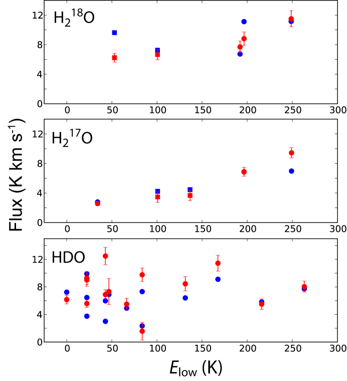
Figure 9: Single-component RADEX models of H₂¹⁸O, H₂¹⁷O, and HDO emission in the Compact Ridge. The common parameters to all three models are: $T_{kin}$ = 125 K, $n$(H₂) = $10^{7}$ cm^-3, $\theta_{s}=6^{\prime\prime}$, and the observed continuum field from Figure 5. The molecular column densities are $N$(H₂¹⁸O) = $4.1\times 10^{15}$ cm^-2 and $N$(HDO) = $3.9\times 10^{15}$ cm^-2. The red points indicate the observed line fluxes, while the blue points indicate the model fluxes. For H₂¹⁸O and H₂¹⁷O, circles indicate ortho transitions, while squares incdicate para. An ortho:para ratio of 3:1 is assumed for H₂¹⁸O and H₂¹⁷O.

3.5 Plateau

The emission and absorption components of the outflow are treated separately in this work. The emissive Plateau component makes up most of the integrated flux in the lower-energy lines (see Figure 2 and 3), and is detected in nearly all lines up to $E_{\textnormal{up}}=500$ K. For this component, we use a source size of $30^{\prime\prime}$ based on a HIFI map of the H₂¹⁶O $2_{12}-1_{01}$ transition (Melnick et al., in preparation). Because this component is detected in so many transitions, we apply the population correction method to derive the column density, estimating the optical depth by comparison of corresponding H₂¹⁸O and H₂¹⁷O transitions as explained above. Many of these H₂¹⁸O transitions have moderate optical depth ($\tau\sim$ 1–2). For the transitions where one of the two isotopologues is not detected due to blends with transitions of other molecules, we assume the usable line is optically thin. To derive a correction factor, we use $T_{\textnormal{kin}}=125$ K, $n$(H₂) = $10^{7}$ cm^-3, and the observed continuum in Figure 5. This yields $f_{c}=2.25$ for ortho-water and 1.80 for para-water, and so derive a total column density $N$(H₂¹⁸O) of $(3.5\pm 0.6)\times 10^{15}$ cm^-2, and an ortho:para ratio of $2.27\pm 0.73$. For HDO, assuming that lines are optically thin, and using the more optically thin transition in cases where two lines are detected with the same upper state, and using a correction factor of 1.6 (derived with the same parameters as for H₂O), a column density $N$(HDO) = $(1.23\pm 0.25)\times 10^{15}$ cm^-2 is found. In the error propagations, we assume a 20% uncertainty in each correction factor.

The absorption component is detected in several low-energy lines of both HDO and H₂O: two transitions ($1_{11}-0_{00}$ and $2_{12}-1_{01}$) of H₂¹⁸O, H₂¹⁷O, and HDO, as well as two higher-energy transitions ($2_{21}-2_{12}$ and $3_{03}-2_{12}$) of H₂¹⁸O. Fits to the eight transitions with a detected absorption component are shown in Figure 10. The line profiles are fit to the following equation (following Melnick et al. (2010)):

$$T_{mb}(v)=(I_{\textnormal{continuum}}+G_{\textnormal{HC}}(v)+G_{\textnormal{CR}}(v)+G_{\textnormal{PL}}(v))e^{-G_{\textnormal{abs}}(v)}$$ (5)

Here, $G_{\textnormal{HC}}$, $G_{\textnormal{CR}}$, and $G_{\textnormal{PL}}$ are Gaussian components corresponding to the three emissive components in Orion KL with the velocity parameters given in Tables 3-5; and $G_{\textnormal{abs}}$ is a Gaussian component corresponding to the absorption component. Melnick et al. (2010) also included in the fits to the line profiles a narrow ($\Delta v=6.7$ km s^-1) absorption component in addition to the broad one used here, but this is only seen in H₂¹⁶O transitions and not in the rare isotopologues so it is not included here. In Figure 11 and Table 6, the intensity of the absorption component is presented as $|\Delta T_{\textnormal{abs}}/T_{\textnormal{bg}}|$, which is equal to $(1-e^{-G_{\textnormal{abs}}})$ at the peak of the absorption component. We assume that both the continuum and the water absorbing layer fill the Herschel beam. For the lines detected in HIFI bands 6 and 7, where the beamwidth is $\sim 12^{\prime\prime}$, spectra were acquired with two pointings, one near the Hot Core peak and the other near the nominal Compact Ridge, separated by $8^{\prime\prime}$. The pointing error in these observations is estimated as $3^{\prime\prime}$. Figure 10 shows that the absorption wing has a very similar intensity and profile in the two pointings. This suggests that the treatment of the absorbing gas as spatially extended is reasonable. In these fits, an LSR velocity of -5.1 km s^-1 and a width of 30 km s^-1 (Melnick et al., 2010) is assumed, and these parameters are not varied in the fit in order to avoid a fit with too many free parameters.

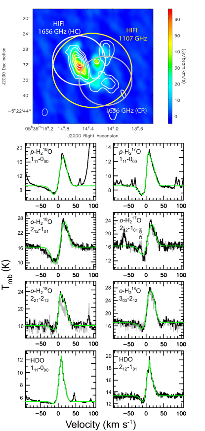
Figure 10: Fits to the transitions of H₂¹⁸O, H₂¹⁷O, and HDO with a detected absorption component. In the top panel, the color scale is the total integrated flux (from 2.8–11.5 km/s) of the $3_{12}-2_{21}$ transition of HDO from ALMA, the white contours are the continuum emission at 230 GHz (same contour levels as in Figure 6). The half-power beamwidth and pointing of the HIFI Orion KL spectrum at 1107 GHz (the approximate frequency of the $1_{11}-0_{00}$ transitions of H₂¹⁸O and H₂¹⁷O) and both the Hot Core (HC) and Compact Ridge (CR) pointings at 1656 GHz (the frequency of the $2_{12}-1_{01}$ transitions) are overlaid. In the lower panels, the green curves are the fits to the transitions following equation (5). For the ortho-H₂¹⁸O and H₂¹⁷O transitions, the black spectrum is the Hot Core pointing, and the gray spectrum is the Compact Ridge pointing. The blue wing of the H₂¹⁷O $2_{12}-1_{01}$ is contaminated by a transition of CH₃OH (the $16_{6}-15_{5}$ of the $E$ torsional subspecies at 1662586.2 MHz). This transition is centered at a velocity of -14 km s^-1 in the reference frame of the H₂¹⁷O transition.

Figure 11 shows model line/continuum ratios for the absorption components under a range of values for $T_{\textnormal{ex}}$ and column density in order to constrain the H₂O and HDO column density. Panel A shows the two detected ground state ($1_{11}-0_{00}$) transitions of para-H₂¹⁸O and H₂¹⁷O. The black lines surround the parameter space where the two transitions are both fit within $1\sigma$, which yield the values $N$(p-H₂¹⁸O) = $2.8_{-1.8}^{+3.4}\times 10^{14}$ cm^-2 and $T_{\textnormal{ex}}$ = $23.2_{-3.4}^{+1.4}$ K. This uncertainty also includes a 20% error due to the uncertainty in the ¹⁸O/¹⁷O ratio. In these calculations, we assume that all energy levels are in LTE at the derived $T_{\textnormal{ex}}$. However, the correction to the total column density located in higher energy levels (i.e., not $0_{00}$ or $1_{11}$) is likely to be small ($\sim$ 10%), so this derivation is not extremely sensitive to non-LTE excitation. For ortho-H₂O, a similar analysis of the $2_{12}-1_{01}$ ground state transitions yields $N$(o-H₂¹⁸O) = $4.2_{-2.7}^{+3.6}\times 10^{14}$ cm^-2 and $T_{\textnormal{ex}}$ = $32.2_{-11.1}^{+3.3}$ K (the black lines in panel B). Meanwhile, looking at the ground state and the two higher-energy H₂¹⁸O lines (the region outlined in gray in panel B), we derive a column density of $9.8_{-1.9}^{+2.2}\times 10^{14}$ cm^-2 and $T_{\textnormal{ex}}$ = $34.7_{-1.5}^{+1.3}$ K. In Figure 11, the $2_{21}-2_{12}$ transition is not plotted; its contours overlap with those of the $3_{03}-2_{12}$ transition within the uncertainties. The average of these two analyses, $N$(ortho-H₂¹⁸O) = $7.0_{-2.3}^{+2.9}\times 10^{14}$ cm^-2, is taken as the best estimate. Unlike for para, there is a low-lying state ($1_{10}$) at $E=26.3$ K above the ground state, so the correction for population in missing levels is more significant ($\sim 30\%$). For HDO (panel C), analysis of the two transitions yields $N$(HDO) = $5.5_{-0.7}^{+0.6}\times 10^{13}$ cm^-2 and $T_{\textnormal{ex}}$ = $16.9_{-0.8}^{+0.8}$ K.

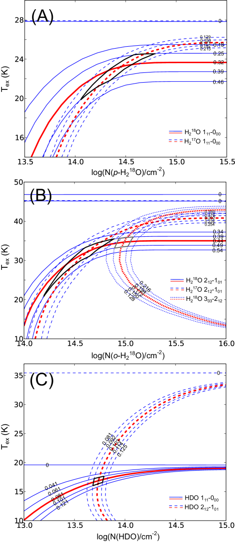
Figure 11: Models to the absorption component of H₂O and HDO. The red contours indicate the absolute value of the fit line/continuum ratio for each transition, while the blue contours indicate the $\pm 1\sigma$ and $\pm 2\sigma$ error bars. The black and gray lines indicate the parameter space where the $\pm 1\sigma$ error bars intersect for two transitions.

D₂O is not detected in either the emission or absorption components of the outflowing gas. As Figure 4 shows, particularly the ground state transitions ($1_{11}-0_{00}$ for ortho, $2_{12}-1_{01}$ for para) are fairly clean in the wings where these components would be detected. Using LTE models, we estimate an upper limit to the [D₂O]/[HDO] ratio of $\sim 0.1$ in both components. A ratio of 0.01 or less would be expected based on the [HDO]/[H₂O] ratio in these components (Table 2).

4 Discussion

We note some differences between the H₂O abundances derived here and those of Melnick et al. (2010), which were derived using the same data set. These differences could arise either in the Gaussian fitting process (i.e., the attribution of the total flux observed by HIFI to the various spatial components) or in the derivation of the water column density from these Gaussian components. The only component strongly affected by differences in the Gaussian fitting is the Compact Ridge, which was fit in a different way between the two analyses. In Melnick et al. (2010), the linewidth for the Gaussians attributed to this component (which was called “extended warm gas”) was allowed to vary between 2–8 km s^-1, which likely encompasses flux belonging to regions not identified with the spatially and spectrally distinct Compact Ridge region. This is the most significant reason for the lower Compact Ridge H₂O abundance derived in this study, though other methodological assumptions also contribute. For the Hot Core and Plateau, on the other hand, the fluxes attributed to these components are similar, within 20% for most transitions.

The Hot Core was modeled as a single component in the previous study, but with two spatial components here, which is largely responsible for the different abundances, and particularly the higher water abundance in the $2^{\prime\prime}$, 7 km s^-1 component. For the emissive Plateau component, we derive a H₂O abundance a factor of 15 lower than that of Melnick et al. (2010). Some of this difference is due to factors connected with the conversion of the H₂¹⁸O column density (the primary quantity derived by the radiative transfer modeling) to a H₂O abundance relative to H₂: a solar ¹⁶O/¹⁸O isotopic ratio of 500 was assumed by Melnick et al. (2010), whereas a value of 250 is used here (Tercero et al., 2010). Additionally, the H₂ column density used for that study was $1.0\times 10^{23}$ cm^-2 from Blake et al. (1987), while we use $1.8\times 10^{23}$ cm^-2 (Plume et al., 2012). Both of these factors lower the H₂O abundance from that of Melnick et al. (2010); however, there is still a factor of 4 difference in the H₂¹⁸O column density that is attributed to differences in the methods used for the column density derivation. The previous analysis did not use H₂¹⁷O transitions as a constraint on the optical depth of the H₂¹⁸O lines. In the analysis presented here, the column density is sensitive only to two factors: the optical depth estimates, and the value of $f_{c}$ used to account for population in unprobed levels. The optical depth estimates depend on the ¹⁸O/¹⁷O ratio, as discussed above, and also assume that $T_{\textnormal{ex}}$ is the same between corresponding transitions of the two isotopologues. RADEX modeling suggests that this may not always be the case, and small deviations (10–20%) from this assumption can cause large uncertainties, a factor of 2 or more, in the population in individual levels. We find that the correction factor is relatively insensitive to physical conditions, and particularly to the intensity of the radiation field; most of the unprobed population is located in the ground state levels, which are not as strongly affected by the far-IR continuum.

The component with highest water abundance is the small $v_{\textnormal{LSR}}=7$ km s^-1 clump within the Hot Core region, where most of the oxygen is in gas-phase water. The other spatial components have lower abundances by about two orders of magnitude (2.7–6.7 $\times 10^{-6}$). This high abundance and the high [HDO]/[H₂O] ratio of 0.003 observed in the 7 km s^-1 Hot Core component (and a comparable [D₂O]/[HDO] ratio of 0.0016) suggest that much of this water is material that has been recently evaported from ice mantles. Low-temperature gas-phase chemistry could produce water with significant deuterium fractionation, for example, through ion-neutral reactions involving H₂D⁺ (Millar et al., 1989), but likely not with such a high water abundance (Herbst & Klemperer, 1973; Woodall et al., 2007). Gas-phase neutral-neutral chemistry in shocked gas, on the other hand, can produce H₂O abundances of $\sim 10^{-4}$ (Draine et al., 1983; Bergin et al., 1998), but not with such high deuterium fractionation due to the high temperatures required (Bergin et al., 1999). The more spatially extended component in the Hot Core (with velocity centered at 5 km s^-1) has a lower abundance of H₂O, but this value is a lower limit. Similar deuterium fractionation is found in the two Hot Core components.

The Compact Ridge has somewhat higher deuteration than the Hot Core, suggesting that H₂O in this region may have been synthesized under slightly colder conditions. The spatial distribution of HDO emission (Figure 6) has an interesting morphology, with the strongest emission found to the northeast of the continuum peak, in the part of the Compact Ridge facing nearest to the Hot Core (and so nearest to the origin of the molecular outflow), rather than where other oxygen-bearing organic species peak; e.g. the MF1 peak in Figure 5 is the region of strongest methyl formate (HCOOCH₃) emission (Favre et al., 2011). The Compact Ridge has been suggested to be a site of recent interaction between the molecular outflow from Source I (Zapata et al., 2012) and pre-existing dense gas, leading to the liberation of organic material from ice mantles (Blake et al., 1987; Liu et al., 2002; Favre et al., 2011). However, physical conditions will also play a role in the excitation of these HDO transitions.

The emission component of the Plateau has a somewhat lower HDO/H₂O ratio than the compact regions, and the absorption component has lower deuterium fractionation by an order of magnitude. This suggests that most of the water in the outflow, and particularly in the absorbing gas, does not have the same origin as the more deuterated water in the Hot Core and Compact Ridge. The HDO/H₂O ratio can be modified in shocks by gas-phase neutral-neutral chemistry (Kaufman & Neufeld, 1996; Bergin et al., 1998, 1999). Water synthesis in shocked gas proceeds by the following mechanism:

$$\textnormal{O}+\textnormal{H}_{2}\rightarrow\textnormal{OH}+\textnormal{H}$$ (6)

$$\textnormal{OH}+\textnormal{H}_{2}\rightarrow\textnormal{H}_{2}\textnormal{O}+\textnormal{H}$$ (7)

HDO can be formed through similar chemistry, with either

$$\textnormal{O}+\textnormal{HD}\rightarrow\textnormal{OD}+\textnormal{H}$$ (8)

or

$$\textnormal{OH}+\textnormal{HD}\rightarrow\textnormal{HDO}+\textnormal{H}$$ (9)

in place of Eq. (5) or (6). Rates for the relevant reactions are available through the UMIST astrochemistry database (Woodall et al., 2007) and in Bergin et al. (1999). These reactions, particularly equations (5) and (7), have substantial energy barriers (e.g., 3160 K for equation (5)). However, in a sufficiently energetic shock, this set of reactions can nevertheless convert all oxygen not in CO into water. For example, in a C-type shock with a velocity of 20 km s^-1, corresponding to a peak gas temperature of 1000 K (Kaufman & Neufeld, 1996), and with an H₂ density of $10^{5}$ cm^-3, the pseudo-first order reaction rate of equation (5) is $3.5\times 10^{-8}$ s^-1. This corresponds to a timescale for the conversion of O to H₂O of 0.9 yr, far shorter than the lifetime of the shock (Bergin et al., 1998), so atomic oxygen will be readily converted to water by these reactions. Equations (7) and (8) have far slower rates, due to the low abundance of HD relative to H₂ ($\sim 2\times 10^{-5}$); under these same conditions, equation (7) has a pseudo-first order rate of $2.3\times 10^{-13}$ s^-1. A kinetic analysis shows that a 20 km s^-1 C-type shock ($T_{\textnormal{gas}}=1000$ K) with an H₂ density of $10^{5}$ cm^-3 and [HD]/[H₂] = $2\times 10^{-5}$ will produce water with [HDO]/[H₂O] = $8\times 10^{-6}$. This is lower than the [HD]/[H₂] ratio due to slower rate constants for the reactions involving deuterium.

The [HDO]/[H₂O] ratios observed both the emission and absorption components of the outflow are intermediate between the ratio observed in the Hot Core and Compact Ridge and the low ratio anticipated by the shock gas-phase water production mechanism. This suggests that the gas in the outflow originated close to the core of Orion KL with a higher HDO/H₂O ratio, possibly similar to the fractionation observed in the quiescent components, and the fractionation has been reduced by the production of additional water in the outflow with a low HDO/H₂O ratio. OH⁺ and H₂O⁺ have been detected in the absorbing layer (Gupta et al., 2010); it was proposed by these authors that these ions could be produced by the photodissociation of H₂O. If water has a substantial destruction rate in the outflow, the original water that originated from ice mantles is destroyed on a relatively short timescale and could be replaced with fresh water with a low HDO/H₂O ratio produced via high-temperature gas-phase chemistry. The deuterium fractionation in outflows could therefore reflect both the physical conditions in the preshocked gas and in the shock itself. Additionally, we note that the H₂O abundance in the outflow ($\sim 3\times 10^{-6}$) is low compared to the ISO studies of Harwit et al. (1998) and Cernicharo et al. (2006), who find beam-averaged H₂O abundances of $2\times 10^{-5}-4\times 10^{-4}$. These analyses were primarily concerned with transitions of the H₂¹⁶O isotopologue, which are significantly broader than those of H₂¹⁸O and H₂¹⁷O, also seen in Melnick et al. (2010), and therefore are probing more of the high-velocity shocks. The present analysis, focusing on rare isotopologues of water, is concerned with the regions of highest water optical depth closer to the KL nebula, which may have lower water abundance relative to H₂ than the faster shocks.

The factor of 6 difference in the D/H ratios between the emission and absorption components of the outflow is intriguing, and significant within the errors in our analysis. For the emission component, the optical depth of the H₂O lines is likely well characterized due to the detection of both H₂¹⁸O and H₂¹⁷O, although violation of the assumption that $T_{\textnormal{ex}}$ is the same for corresponding H₂¹⁸O and H₂¹⁷O transitions may add uncertainty. Line optical depths are less well chracterized for HDO, but if the opacity has been underestimated the effect will be to increase, rather than decrease, the D/H ratio in the emitting gas. This suggests a chemical difference between the emissive gas of the Plateau and the absorbing layer.

5 Conclusion

Using the HIFI fullband survey of Orion KL, acquired as part of the HEXOS key program, we have detected numerous transitions of isotopologues of H₂O (H₂¹⁸O, H₂¹⁷O, HDO, HD¹⁸O, and D₂O) with a variety of excitation conditions. We have derived abundances of H₂O and HDO in each of the spatial components within this region. Water has a complex morphology in Orion KL, with significant H₂O and HDO emission in the Hot Core, Compact Ridge, and Plateau, as well as absorption in the blue-shifted wing of the outflow in a few low-energy transitions. Both the H₂O abundance and HDO/H₂O ratio have significant differences between spatial components, and we propose some possible explanations for these variations. Of particular interest is the small ($2^{\prime\prime}$) clump we identify in the Hot Core region, which we attribute to a region just south of the dust continuum peak, and near (but not coincident with) the SMA1 submillimeter continuum peak of Beuther et al. (2004). This region has a very high abundance of water, with a high [HDO]/[H₂O] ratio (0.003), suggesting material that was formed at low temperatures and has been recently evaporated from ice mantles. This region also shows signs of significant excitation from a nearby far-IR field, possibly from an embedded far-IR continuum source, in agreement with the recent study of H₂S in the Hot Core (Crockett et al. 2013a, in preparation). The far-IR dust opacity is likely to be very high in this region, which make continuum sources difficult to detect directly. Further investigations into the spatial distributions of transitions of molecules that trace the far-IR radiation field will be crucial in investigating the physical structure of this region.

Appendix A Fit line parameters for H₂O isotopologues

Table 3: Fit integrated fluxes for H₂O isotopologues in the Hot Core.

Transition	Frequency	$E_{u}$	$S_{\textnormal{ij}}\mu^{2}$	$\int T_{\textnormal{mb}}dv$	$v_{\textnormal{LSR}}$	$\Delta v$
	(MHz)	(K)	(D2)	(K km s-1)	(km s-1)	(km s-1)
H218O
$2_{02}-1_{11}$	994675.1	100.6	2.63	48.7(5.7)	5.2	10.0
$2_{11}-2_{02}$	745320.2	136.4	7.09	37.1(4.3)	5.2	10.0
$2_{21}-2_{12}$	1633483.6	192.0	8.60	40.2(6.5)	5.2	10.0
$3_{03}-2_{12}$	1719250.2	196.2	18.16	22.4(6.1)	5.2	10.0
$3_{12}-2_{21}$	1181394.0	248.7	3.17	62.2(6.4)	3.6(0.1)	8.9(0.1)
$3_{12}-3_{03}$	1095627.4	248.7	22.24	56.1(6.8)	3.6(0.2)	9.6(0.4)
$3_{22}-3_{13}$	1894323.8	294.6	4.45	49.3(7.0)	4.9(0.2)	8.1(0.6)
$3_{21}-3_{12}$	1136703.6	303.3	26.42	56.9(5.7)	5.2	10.0
$4_{13}-4_{04}$	1605962.5	395.4	6.93	38.3(7.6)	4.87(0.2)	6.4(0.8)
$4_{22}-4_{13}$	1188863.1	452.4	12.55	80.6(8.9)	5.2	10.0
$5_{24}-4_{31}$	1003277.6	595.9	0.90	9.0(1.0)	5.6(0.1)	6.7(0.3)
$5_{32}-4_{41}$	692079.1	727.6	1.26	4.3(0.5)	5.2	8.2(0.4)
$5_{32}-5_{23}$	1815853.4	727.6	35.87	70.7(7.5)	5.8(0.2)	9.0(0.4)
$6_{24}-6_{15}$	1800474.6	865.0	14.35	30.0(3.5)	3.5(0.2)	7.2(0.5)
$6_{34}-5_{41}$	1216850.4	928.6	2.92	8.8(1.0)	5.3(0.3)	10.0
$6_{33}-5_{42}$	1620851.6	947.6	1.08	27.6(3.9)	4.1(0.5)	10.4(1.3)
$7_{34}-7_{25}$	1771674.6	1207.9	61.01	14.9(3.4)	5.7(0.6)	6.7(1.8)
H217O
$1_{11}-0_{00}$	1107166.9	53.1	3.44	29.7(3.8)	5.2	10.0
$1_{10}-1_{01}$	552021.0	60.7	15.48	6.6(0.9)	5.2	10.0
$2_{11}-2_{02}$	748458.3	136.6	7.11	37.3(17.6)	5.2	10.0
$2_{21}-2_{12}$	1646398.7	193.0	8.60	27.5(6.3)	5.2	10.0
$2_{20}-2_{11}$	1212980.4	194.9	4.36	26.2(3.9)	5.2	10.0
$3_{03}-2_{12}$	1718119.5	196.5	18.08	54.5(9.1)	5.2	10.0
$3_{12}-3_{03}$	1096414.3	249.1	22.38	57.6(5.8)	3.7(0.1)	10.0
$3_{21}-3_{12}$	1148976.1	304.2	26.31	57.5(6.2)	4.2(0.2)	10.0
$4_{13}-4_{04}$	1604179.9	395.9	6.98	42.0(11.9)	5.3(0.3)	8.8(1.3)
$4_{22}-4_{13}$	1197610.3	453.3	12.54	33.8(6.8)	5.1(0.7)	7.9(2.3)
$5_{32}-5_{23}$	1840155.7	729.7	35.63	32.2(4.0)	5.7(0.3)	7.0(0.6)
$6_{24}-6_{15}$	1797675.5	866.1	14.47	16.0(4.3)	5.2(0.7)	7.5(2.2)
$7_{34}-7_{25}$	1783388.8	1209.8	60.99	9.6(3.5)	7.2(1.2)	7.2(2.9)
HDO
$1_{11}-0_{00}$	893638.7	42.9	3.0	23.8(3.4)	5.2	10.0
$1_{10}-1_{01}$	509292.4	46.8	4.52	11.4(2.8)	5.2	10.0
$2_{02}-1_{01}$	919310.9	66.4	0.86	44.6(4.5)	5.2	10.0
$2_{02}-1_{11}$	490596.6	66.4	1.91	14.3(1.5)	5.0	10.0
$2_{12}-1_{01}$	1277675.9	83.6	4.53	27.7(2.9)	5.2	10.0
$2_{12}-1_{11}$	848961.8	83.6	0.65	24.5(2.5)	5.2	10.0
$2_{11}-1_{10}$	1009944.7	95.2	0.65	45.9(7.0)	5.2	10.0
$2_{11}-2_{02}$	599926.7	95.2	6.87	30.0(3.1)	6.5(0.5)	11.3(0.5)
$3_{03}-2_{12}$	995411.5	131.4	4.30	43.6(4.5)	5.2	10.0
$3_{13}-2_{02}$	1625408.1	144.4	6.29	24.1(7.5)	6.6(0.8)	10.0
$2_{21}-2_{12}$	1522925.8	156.7	2.51	18.6(3.1)	2.9(0.8)	10.0
$3_{12}-2_{11}$	1507261.0	167.6	1.16	35.6(4.7)	4.3(0.4)	10.0
$3_{12}-3_{03}$	753411.2	167.6	8.30	39.0(5.7)	5.2	10.0
$4_{04}-3_{13}$	1491926.9	216.0	7.15	22.9(4.4)	5.2	10.0
$3_{22}-3_{13}$	1648801.4	223.6	4.13	50.3(5.7)	5.2	10.0
$4_{14}-3_{13}$	1678577.8	225.0	1.62	29.4(5.7)	4.9(0.3)	7.1(0.9)
$3_{21}-2_{20}$	1432876.7	226.0	0.72	45.5(9.9)	6.3(1.0)	10.2(2.4)
$3_{21}-3_{12}$	1217258.3	226.0	6.33	48.1(9.0)	4.5(0.3)	10.6(0.7)
$4_{13}-4_{04}$	984137.8	263.3	8.75	56.4(5.7)	5.3(0.3)	10.0
$4_{13}-3_{22}$	827263.4	263.3	1.75	28.5(3.0)	5.8(0.1)	8.4(0.2)
$4_{23}-3_{22}$	1848306.0	312.3	1.30	40.7(4.7)	4.4(0.2)	8.5(0.6)
$4_{23}-4_{14}$	1818529.7	312.3	5.30	32.9(7.6)	4.8(0.3)	9.1(1.2)
$4_{22}-4_{13}$	1164769.9	319.2	9.81	63.7(6.8)	5.2	10.0
$5_{14}-4_{23}$	1444829.0	381.6	3.21	26.9(7.5)	3.7(0.9)	6.9(2.1)
$5_{14}-5_{15}$	1180323.5	381.6	0.17	11.5(1.2)	5.8(1.3)	6.8(0.4)
$4_{32}-3_{31}$	1872608.6	425.1	0.76	26.7(3.4)	5.4(0.3)	7.5(0.7)
$4_{31}-3_{30}$	1877486.8	425.4	0.76	18.0(2.9)	5.6(0.4)	6.3(1.0)
$6_{15}-6_{06}$	1684605.8	521.6	8.12	56.5(6.8)	4.7(0.3)	12.0(1.2)
$6_{24}-6_{15}$	1230402.9	580.6	15.82	47.0(5.0)	5.2(0.1)	8.1(0.2)
$6_{24}-5_{33}$	895874.4	580.6	1.78	12.1(1.2)	5.9(0.1)	6.6(0.1)
$7_{26}-6_{33}$	622482.6	705.6	1.65	2.3(0.6)	5.9	5.4(1.0)
$7_{25}-6_{34}$	1577177.6	748.3	2.74	19.3(3.9)	6.8(0.6)	6.3(1.2)
$7_{34}-7_{25}$	1853872.8	837.3	14.83	21.6(2.8)	5.3(0.3)	6.6(0.7)
$8_{27}-7_{34}$	838953.3	877.6	1.71	3.8(1.5)	5.8(1.0)	5.4(2.6)
$8_{26}-8_{17}$	1634639.2	939.6	17.45	16.3(2.9)	6.1(0.5)	5.9(1.1)
$8_{35}-8_{26}$	1759978.4	1024.1	18.77	24.5(4.9)	4.6(0.5)	6.5(1.3)
$9_{36}-9_{27}$	1731255.8	1236.5	22.42	7.4(1.4)	6.2(0.3)	3.1(0.6)
HD18O
$1_{11}-0_{00}$	883189.4	42.4	2.98	3.0(0.4)	6.6(0.2)	5.7(0.4)
$2_{02}-1_{11}$	492814.5	66.0	1.89	0.4(0.2)	6.6(1.0)	4.7(1.0)
$2_{11}-2_{02}$	592405.7	94.5	6.78	2.1(0.4)	7.0(0.6)	6.9(1.4)
$3_{03}-2_{12}$	994348.0	130.6	4.27	4.9(0.9)	7.0(1.0)	6.9(1.4)
$3_{12}-3_{03}$	746475.6	166.4	8.16	1.5(0.3)	6.3(1.3)	4.4(1.1)
$4_{22}-4_{13}$	1144046.2	316.5	9.74	2.1(0.5)	6.9(0.5)	4.6(0.4)
D2O
$1_{11}-0_{00}$	607349.5	29.1	6.81	1.08(0.12)	7.6(0.1)	5.5(0.3)
$2_{12}-1_{01}$	897947.1	60.5	5.11	3.3(0.4)	7.7(0.1)	4.6(0.3)
$2_{20}-2_{11}$	743563.4	106.7	7.97	1.02(0.18)	7.0(0.4)	4.8(0.8)
$3_{13}-2_{02}$	1158044.9	107.2	14.48	1.54(0.24)	6.1(0.2)	3.2(0.4)
$3_{21}-3_{12}$	697922.7	161.5	8.07	1.6(0.5)	8.7(0.6)	4.8(1.7)
$4_{13}-4_{04}$	782470.9	203.0	16.02	0.60(0.07)	8.0(0.1)	3.2(0.3)

Table 4: Fit integrated fluxes for H₂O isotopologues in the Compact Ridge.

Transition	Frequency	$E_{u}$	$S_{\textnormal{ij}}\mu^{2}$	$\int T_{\textnormal{mb}}dv$	$v_{\textnormal{LSR}}$	$\Delta v$
	(MHz)	(K)	(D2)	(K km s-1)	(km s-1)	(km s-1)
H218O
$2_{02}-1_{11}$	994675.1	100.6	2.63	6.2(1.1)	8.0	3.0
$2_{11}-2_{02}$	745320.2	136.4	7.09	6.7(0.9)	8.0	3.0
$3_{12}-2_{21}$	1181394.0	248.7	3.17	7.7(0.9)	7.6(0.1)	3.0
$3_{12}-3_{03}$	1095627.4	248.7	22.24	8.8(1.3)	7.7(0.1)	3.0
$3_{21}-3_{12}$	1136703.6	303.3	26.42	11.5(1.2)	8.0	3.0
H217O
$1_{10}-1_{01}$	552021.0	60.7	15.48	2.6(0.3)	9.2(1.0)	3.0
$2_{11}-2_{02}$	748458.3	136.6	7.11	3.5(1.0)	7.7(0.8)	2.6(0.4)
$2_{20}-2_{11}$	1212980.4	194.9	4.36	3.6(1.0)	9.0	3.0
$3_{12}-3_{03}$	1096414.3	249.1	22.38	6.9(0.8)	7.6(0.8)	3.0
$3_{21}-3_{12}$	1148976.1	304.2	26.31	9.4(1.4)	8.2(0.8)	3.0
HDO
$1_{11}-0_{00}$	893638.7	42.9	3.0	6.2(0.8)	9.6(0.1)	3.0
$1_{10}-1_{01}$	509292.4	46.8	4.52	5.6(0.8)	9.4(0.2)	3.0
$2_{02}-1_{01}$	919310.9	66.4	0.86	9.0(0.9)	8.6(0.1)	3.0
$2_{02}-1_{11}$	490596.6	66.4	1.91	12.4(1.3)	8.6(0.1)	3.0
$2_{12}-1_{01}$	1277675.9	83.6	4.53	9.3(1.3)	10.2(0.5)	3.0
$2_{12}-1_{11}$	848961.8	83.6	0.65	6.9(0.8)	8.2(0.1)	3.0
$2_{11}-1_{10}$	1009944.7	95.2	0.65	7.3(2.0)	7.9(0.4)	3.0
$2_{11}-2_{02}$	599926.7	95.2	6.87	5.5(1.0)	8.7(0.5)	3.0
$3_{03}-2_{12}$	995411.5	131.4	4.30	9.8(1.0)	8.2(0.1)	3.0
$2_{21}-2_{12}$	1522925.8	156.7	2.51	1.6(0.5)	8.0	3.0
$3_{12}-3_{03}$	753411.2	167.6	8.30	8.4(1.3)	8.0	3.0
$3_{21}-3_{12}$	1217258.3	226.0	6.33	11.4(1.4)	8.0	3.0
$4_{13}-4_{04}$	984137.8	263.3	8.75	5.5(0.9)	8.1(0.3)	3.0
$4_{22}-4_{13}$	1164769.9	319.2	9.81	8.0(1.0)	7.9(0.1)	2.2(0.1)

Table 5: Fit integrated fluxes for H₂O isotopologues in the Plateau (emission component).

Transition	Frequency	$E_{u}$	$S_{\textnormal{ij}}\mu^{2}$	$\int T_{\textnormal{mb}}dv$	$v_{\textnormal{LSR}}$	$\Delta v$
	(MHz)	(K)	(D2)	(K km s-1)	(km s-1)	(km s-1)
H218O
$1_{11}-0_{00}$	1101698.3	52.9	3.44	288(64)	12.1(0.1)	24.9(0.2)
$1_{10}-1_{01}$	547676.4	60.5	15.49	169(17)	12.2(0.2)	25.4(0.5)
$2_{02}-1_{11}$	994675.1	100.6	2.63	380(38)	11.4(0.1)	28.7(0.3)
$2_{12}-1_{01}$	1655867.6	113.7	15.49	405(41)	14.0(0.2)	27.0(0.3)
$2_{11}-2_{02}$	745320.2	136.4	7.09	272(27)	10.6(0.2)	27.3(0.2)
$2_{21}-2_{12}$	1633483.6	192.0	8.60	161.4(16.6)	13.8(0.4)	25.0(0.6)
$3_{03}-2_{12}$	1719250.2	196.2	18.16	271.5(27.6)	14.1(0.3)	22.6(0.4)
$3_{12}-2_{21}$	1181394.0	248.7	3.17	257(26)	9.2(0.1)	25.8(0.1)
$3_{12}-3_{03}$	1095627.4	248.7	22.24	436(44)	10.8(0.1)	27.5(0.2)
$3_{22}-3_{13}$	1894323.8	294.6	4.45	66.7(9.0)	11.9(1.0)	25.0
$3_{21}-3_{12}$	1136703.6	303.3	26.42	494(49)	10.8(0.1)	28.5(0.1)
$4_{13}-4_{04}$	1605962.5	395.4	6.93	73.3(10.5)	8.2(1.1)	23.4(1.8)
$4_{22}-4_{13}$	1188863.1	452.4	12.55	159.8(16.5)	6.7(0.2)	21.9(0.5)
H217O
$1_{11}-0_{00}$	1107166.9	53.1	3.44	102.3(10.3)	13.7(0.5)	23.6(0.8)
$1_{10}-1_{01}$	552021.0	60.7	15.48	96.4(9.7)	11.9(0.1)	26.7(0.2)
$2_{12}-1_{01}$	1662464.4	114.0	15.48	204.5(20.8)	13.6(0.2)	22.5(0.4)
$2_{11}-2_{02}$	748458.3	136.6	7.11	128(26)	9.4(2.0)	25.0
$2_{21}-2_{12}$	1646398.7	193.0	8.60	112.4(13.3)	15.1(0.9)	25.0
$2_{20}-2_{11}$	1212980.4	194.9	4.36	104.6(11.1)	11.0(0.4)	23.7(0.8)
$3_{03}-2_{12}$	1718119.5	196.5	18.08	125.5(15.5)	16.3(1.1)	25.0
$3_{12}-3_{03}$	1096414.3	249.1	22.38	223.8(22.4)	9.7(0.1)	25.0
$3_{21}-3_{12}$	1148976.1	304.2	26.31	220(22)	10.3(0.2)	25.0
$4_{13}-4_{04}$	1604179.9	395.9	6.98	36.4(11.6)	12.7(5.4)	25.0
$4_{22}-4_{13}$	1197610.3	453.3	12.54	67.2(25.3)	5.5(1.5)	17.8(6.8)
HDO
$1_{11}-0_{00}$	893638.7	42.9	3.0	120.7(12.1)	8.4(0.1)	23.0(0.2)
$1_{10}-1_{01}$	509292.4	46.8	4.52	60.4(6.7)	9.1(0.4)	21.0(0.9)
$2_{02}-1_{01}$	919310.9	66.4	0.86	90.2(9.0)	9.6(0.1)	20.6(0.1)
$2_{02}-1_{11}$	490596.6	66.4	1.91	62.0(6.2)	8.6(0.1)	18.6(0.1)
$2_{12}-1_{01}$	1277675.9	83.6	4.53	99.7(10.0)	10.1(0.2)	23.2(0.2)
$2_{12}-1_{11}$	848961.8	83.6	0.65	70.0(7.1)	8.0(0.1)	18.0(0.3)
$2_{11}-1_{10}$	1009944.7	95.2	0.65	74.1(10.1)	9.0	19.0
$2_{11}-2_{02}$	599926.7	95.2	6.87	53.2(5.4)	9.2(0.5)	19.3(0.5)
$3_{03}-2_{12}$	995411.5	131.4	4.30	110.0(11.0)	8.6(0.1)	21.8(0.2)
$3_{13}-2_{02}$	1625408.1	144.4	6.29	51.9(11.2)	9.0	20.0
$2_{21}-2_{12}$	1522925.8	156.7	2.51	61.3(7.1)	9.0	20.0
$3_{12}-2_{11}$	1507261.0	167.6	1.16	44.1(6.0)	9.0	20.0
$3_{12}-3_{03}$	753411.2	167.6	8.30	104.7(11.3)	9.2(0.4)	22.4(0.9)
$4_{04}-3_{13}$	1491926.9	216.0	7.15	72.7(8.8)	11.2(0.9)	25.9(1.5)
$4_{14}-3_{13}$	1678577.8	225.0	1.62	25.3(6.6)	11.9(2.9)	25.0
$3_{21}-3_{12}$	1217258.3	226.0	6.33	77.0(10.5)	9.5(0.7)	22.5(1.1)
$4_{13}-3_{22}$	827263.4	263.3	1.75	19.7(2.1)	5.8(0.4)	16.9(0.8)
$4_{23}-4_{14}$	1818529.7	312.3	5.30	27.8(7.9)	10.5(1.9)	21.0
$4_{22}-4_{13}$	1164769.9	319.2	9.81	79.7(8.3)	7.4(0.2)	22.0(0.6)
$6_{24}-6_{15}$	1230402.9	580.6	15.82	40.4(4.6)	7.5(0.3)	21.0

Table 6: Fit integrated fluxes for H₂O isotopologues in the absorbing gas.

Transition	Frequency	$E_{l}$	$S_{\textnormal{ij}}\mu^{2}$	$\Delta T_{\textnormal{abs}}$	$|\Delta T_{\textnormal{abs}}/T_{\textnormal{bg}}|$	$v_{\textnormal{LSR}}$	$\Delta v$
	(MHz)	(K)	(D2)	(K)		(km s-1)	(km s-1)
H218O
$1_{11}-0_{00}$	1101698.3	0.0	3.44	-2.9(0.6)	0.32(0.07)	-5.1	30.0
$2_{12}-1_{01}$	1655867.6	34.2	15.49	-7.3(0.8)	0.44(0.05)	-5.1	30.0
$2_{21}-2_{12}$	1633483.6	113.7	8.60	-1.52(0.25)	0.092(0.015)	-5.1	30.0
$3_{03}-2_{12}$	1719250.2	113.7	18.16	-2.94(0.37)	0.172(0.022)	-5.1	30.0
H217O
$1_{11}-0_{00}$	1107166.9	0.0	3.44	-1.59(0.19)	0.171(0.021)	-5.1	30.0
$2_{12}-1_{01}$	1662464.4	34.2	15.48	-3.33(0.44)	0.202(0.026)	-5.1	30.0
HDO
$1_{11}-0_{00}$	893638.7	0.0	3.02	-0.44(0.11)	0.081(0.020)	-5.1	25.0
$2_{12}-1_{01}$	1277675.9	22.3	4.53	-1.36(0.14)	0.103(0.011)	-5.1	25.0

References

- Baldwin et al. (1991) Baldwin, J., Ferland, G., Martin, P., et al. 1991, ApJ, 374, 580
- Bally et al. (2011) Bally, J., Cunningham, N., Moeckel, N., et al. 2011, ApJ, 727, 113
- Bellet & Steenbeckeliers (1970) Bellet, J., & Steenbeckeliers, G. 1970, Compt. Rend. Acad. Sci., 271B, 1208
- Benedict et al. (1970) Benedict, W., Clough, S., Frenkel, L., & Sullivan, T. 1970, JChPh, 53, 2565
- Bergin et al. (1998) Bergin, E., Melnick, G., & Neufeld, D. 1998, ApJ, 499, 777
- Bergin et al. (1999) Bergin, E., Neufeld, D., & Melnick, G. 1999, ApJ, 510, L145
- Bergin & van Dishoeck (2012) Bergin, E., & van Dishoeck, E. 2012, RSPTA, 370, 2778
- Bergin et al. (2010) Bergin, E., Phillips, T., Comito, C., et al. 2010, A&A, 521, L20
- Beuther et al. (2004) Beuther, H., Zhang, Q., Greenhill, L., et al. 2004, ApJ, 616, L31
- Blake et al. (1996) Blake, G., Mundy, L., Carlstrom, J., et al. 1996, ApJ, 472, L49
- Blake et al. (1987) Blake, G., Sutton, E., Masson, C., & Phillips, T. 1987, ApJ, 315, 621
- Bockelée-Morvan et al. (1998) Bockelée-Morvan, D., Gautier, D., Lis, D., et al. 1998, Icarus, 133, 147
- Brouillet et al. (2013) Brouillet, N., Despois, D., Baudry, A., et al. 2013, A&A, 550, A46
- Butner et al. (2007) Butner, H., Charnley, S., Ceccarelli, C., et al. 2007, ApJ, 659, L137
- Caselli & Ceccarelli (2012) Caselli, P., & Ceccarelli, C. 2012, A&AR, 20, 56
- Cernicharo et al. (1994) Cernicharo, J., Gonzalez-Alfonso, E., Alcolea, J., Bachiller, R., & John, D. 1994, ApJ, 432, L59
- Cernicharo et al. (1999) Cernicharo, J., Pardo, J., Gonzalez-Alfonso, E., et al. 1999, ApJ, 520, L131
- Cernicharo et al. (1990) Cernicharo, J., Thum, C., Hein, H., et al. 1990, A&A, 231, L15
- Cernicharo et al. (2006) Cernicharo, J., Goicoechea, J., Daniel, F., et al. 2006, ApJ, 649, L33
- Crockett et al. (2010) Crockett, N., Bergin, E., Wang, S., et al. 2010, A&A, 521, L21
- Daniel et al. (2011) Daniel, F., Dubernet, M.-L., & Grosjean, A. 2011, A&A, 536, 76
- de Graauw et al. (2010) de Graauw, T., Helmich, F., Phillips, T., et al. 2010, A&A, 518, L6
- De Lucia & Helminger (1975) De Lucia, F., & Helminger, P. 1975, JMoSp, 56, 138
- De Lucia et al. (1972) De Lucia, F., Helminger, P., Cook, R., & Gordy, W. 1972, PhRvA, 6, 1324
- Draine et al. (1983) Draine, B., Roberge, W., & Dalgarno, A. 1983, ApJ, 264, 485
- Dyke & Muenter (1973) Dyke, T., & Muenter, J. 1973, JChPh, 59, 3125
- Faure et al. (2012) Faure, A., Wisenfeld, L., Scribano, Y., & Ceccarelli, C. 2012, MNRAS, 420, 699
- Favre et al. (2011) Favre, C., Despois, D., Brouillet, N., et al. 2011, A&A, 532, 32
- Friedel & Snyder (2008) Friedel, D., & Snyder, L. 2008, ApJ, 672, 962
- Genzel et al. (1981) Genzel, R., Reid, M., Moran, J., & Downes, D. 1981, ApJ, 244, 884
- Genzel & Stutzki (1989) Genzel, R., & Stutzki, J. 1989, ARA&A, 27, 41
- Gibb et al. (2004) Gibb, E., Whittet, D., Boogert, A., & Tielens, A. 2004, ApJS, 151, 35
- Goldsmith et al. (1997) Goldsmith, P., Bergin, E., & Lis, D. 1997, ApJ, 491, 615
- Goldsmith & Langer (1999) Goldsmith, P., & Langer, W. 1999, ApJ, 517, 209
- Greenhill et al. (1998) Greenhill, L., Gwinn, C., Schwartz, C., Moran, J., & Diamond, P. 1998, Nature, 396, 650
- Guélin et al. (2008) Guélin, M., Brouillet, N., Cernicharo, J., Combes, F., & Wootten, A. 2008, Ap&SS, 313, 45
- Gupta et al. (2010) Gupta, H., Rimmer, P., Pearson, J., et al. 2010, A&A, 521, L47
- Hartogh et al. (2011) Hartogh, P., Lis, D., Bockelée-Morvan, D., et al. 2011, Nature, 478, 218
- Harwit et al. (1998) Harwit, M., Neufeld, D., Melnick, G., & Kaufman, M. 1998, ApJ, 497, L105
- Herbst & Klemperer (1973) Herbst, E., & Klemperer, W. 1973, ApJ, 185, 505
- Herbst & van Dishoeck (2009) Herbst, E., & van Dishoeck, E. 2009, ARA&A, 47, 427
- Hermsen et al. (1988) Hermsen, W., Wilson, T., Walmsley, C., & Henkel, C. 1988, A&A, 201, 285
- Hirota et al. (2012) Hirota, T., Kim, M., & Honma, M. 2012, ApJL, 757, 1
- Jacq et al. (1990) Jacq, T., Walmsley, C., Henkel, C., et al. 1990, A&A, 228, 447
- Johns (1985) Johns, J. 1985, JOSAB, 2, 1340
- Kaufman & Neufeld (1996) Kaufman, M., & Neufeld, D. 1996, ApJ, 456, 611
- Lerate et al. (2006) Lerate, M., Barlow, M., Swinyard, B., et al. 2006, MNRAS, 370, 597
- Liu et al. (2002) Liu, S.-Y., Girart, J., Remijan, A., & Snyder, L. 2002, ApJ, 576, 255
- Lovas (1978) Lovas, F. 1978, JPCRD, 7, 1445
- Melnick (2009) Melnick, G. 2009, ASP Conf. Ser., 417, 59
- Melnick et al. (2000) Melnick, G., Ashby, M., Plume, R., et al. 2000, ApJ, 539, L87
- Melnick et al. (2010) Melnick, G., Tolls, V., Neufeld, D., et al. 2010, A&A, 521, L27
- Menten et al. (1990) Menten, K., Melnick, G., Phillips, T., & Neufeld, D. 1990, ApJ, 363, L27
- Menten & Reid (1995) Menten, K., & Reid, M. 1995, ApJ, 445, L157
- Menten et al. (2007) Menten, K., Reid, M., Forbrich, J., & Brunthaler, A. 2007, A&A, 474, 515
- Messer et al. (1984) Messer, J., De Lucia, F., & Helminger, P. 1984, JMoSp, 105, 139
- Millar (2003) Millar, T. 2003, SSRv, 106, 73
- Millar et al. (1989) Millar, T., Bennett, A., & Herbst, E. 1989, ApJ, 340, 906
- Müller et al. (2005) Müller, H., Sclöder, F., Stutzki, J., & Winnewisser, G. 2005, JMoSt, 742, 215
- Müller et al. (2001) Müller, H., Thorwirth, S., Roth, D., & Winnewisser, G. 2001, A&A, 370, L49
- Neill et al. (2011) Neill, J., Steber, A., Muckle, M., et al. 2011, JPCA, 115, 6472
- Neufeld et al. (1995) Neufeld, D., Lepp, S., & Melnick, G. 1995, ApJS, 100, 132
- Nissen et al. (2012) Nissen, H., Cunningham, N., Gustafsson, M., et al. 2012, A&A, 540, A119
- Öberg et al. (2011) Öberg, K., Boogert, A., Pontoppidan, K., et al. 2011, ApJ, 740, 109
- Ott (2010) Ott, S. 2010, ASP Conference Ser., 434, 139
- Pardo et al. (2001) Pardo, J., Cernicharo, J., Herpin, F., et al. 2001, ApJ, 562, 799
- Persson et al. (2007) Persson, C., Olofsson, A., Koning, N., et al. 2007, A&A, 476, 807
- Petuchowski & Bennett (1988) Petuchowski, S., & Bennett, C. 1988, ApJ, 326, 376
- Phillips et al. (2010) Phillips, T., Bergin, E., Lis, D., et al. 2010, A&A, 518, L109
- Pickett et al. (1998) Pickett, H., Poynter, I., Cohen, E., et al. 1998, JQSRT, 60, 883
- Pilbratt et al. (2010) Pilbratt, G., Riedinger, J., Passvogel, T., et al. 2010, A&A, 518, L1
- Plume et al. (2012) Plume, R., Bergin, E., Phillips, T., et al. 2012, ApJ, 744, 28
- Roelfsema et al. (2012) Roelfsema, P., Helmich, F., Teyssier, D., et al. 2012, A&A, 537, A17
- Rubin et al. (1991) Rubin, R., Simpson, J., Haas, M., & Erickson, E. 1991, ApJ, 374, 564
- Schöier et al. (2005) Schöier, F., van der Tak, F., van Dishoeck, E., & Black, J. 2005, A&A, 432, 369
- Steenbeckeliers & Bellet (1971) Steenbeckeliers, G., & Bellet, J. 1971, Compt. Rend. Acad. Sci., 273B, 471
- Steenbeckeliers & Bellet (1973) —. 1973, JMoSp, 45, 10
- Tercero et al. (2010) Tercero, B., Cernicharo, J., Pardo, J., & Goicoechea, J. 2010, A&A, 517, 96
- Turner et al. (1975) Turner, B., Fourikis, N., Morris, M., Palmer, P., & Zuckerman, B. 1975, ApJ, 198, L125
- van der Tak et al. (2007) van der Tak, F., Black, J., Schöier, F., Jansen, D., & van Dishoeck, E. 2007, A&A, 468, 627
- van Dishoeck et al. (1998) van Dishoeck, E., Wright, C., Cernicharo, J., et al. 1998, ApJ, 502, L173
- van Dishoeck et al. (2011) van Dishoeck, E., Kristensen, L., Benz, A., et al. 2011, PASP, 123, 138
- Vastel et al. (2010) Vastel, C., Ceccarelli, C., Caux, E., et al. 2010, A&A, 521, L31
- Wang et al. (2011) Wang, S., Bergin, E., Crockett, N., et al. 2011, A&A, 527, 95
- Wilson & Rood (1994) Wilson, T., & Rood, R. 1994, ARA&A, 32, 191
- Woodall et al. (2007) Woodall, J., Agúndez, M., Markwick-Kemper, A., & Millar, T. 2007, A&A, 466, 1197
- Zapata et al. (2012) Zapata, L., Rodriguez, L., & Schmid-Burgk, J. 2012, ApJ, 754, L17
- Zapata et al. (2011) Zapata, L., Schmid-Burgk, J., & Menten, K. 2011, A&A, 529, 24