Free energy potential and temperature with information exchange

Abstract

In this paper we develop a generalized formalism for equilibrium thermodynamic systems when an information is shared between the system and the reservoir. The information results in a correction to the entropy of the system. This extension of the formalism requires a consistent generalization of the concept of thermodynamic temperature. We show that this extended equilibrium formalism includes also non-equilibrium conditions in steady state. By non-equilibrium conditions we mean here a non Boltzmann probability distribution within the phase space of the system. It is in fact possible to map non-equilibrium steady state in an equivalent system in equilibrium conditions (Boltzmann distribution) with generalized temperature and the inclusion of the information potential corrections. A simple model consisting in a single free particle is discussed as elementary application of the theory.

PACS numbers

May be entered using the \pacs{#1} command.

In the last fifty years, a big effort has been devoted in trying to extend the thermodynamic formalism beyond equilibrium conditions crooksthesis ; jarzynski4 ; crooks4 ; boksen ; muschik2 ; crooks2 ; crooks3 ; zubarev2 ; luzzi1 . Similar studies have been carried out about the definition of a non-equilibrium temperature diventra ; tempneq . Moreover, our civilization is going in the direction of diffuse information sharing where information technology is ubiquitous. The inclusion of information sharing effects within conventional thermodynamic systems is then of paramount relevance sagawa2 ; sagawa3 .

In this work we present a formalism to extend the concept of free energy when, beside heat or particles, the system exchanges also information with the reservoir alessio . The extension of the formalism requires a consistent generalization of the concept of thermodynamic temperature. The sharing of information between system and reservoir can be interpreted as the presence of a Maxwell Demon which is able to reduce the internal entropy of the system. The formalism can be also extended to include steady state non equilibrium systems where the probability distribution (PD) within phase space does not follow Boltzmann distribution.

Information is the central quantity in our work and it is already present within the definition of conventional entropy. Entropy $S$ is an extensive quantity which measures the internal disorder of the system: $S=-k\int p(\vec{x})\ln\left(p(\vec{x})\right)d\vec{x}$, where $k$ is the Boltzmann constant and $p(\vec{x})$ the probability of the system to be in the $\vec{x}^{th}$ microstate. Every microstate configuration has a well defined energy $\mathcal{E}(\vec{x})$, where $\mathcal{E}(\vec{x})$ is the Hamiltonian of the system. The nature of $\vec{x}$ degrees of freedom depend on the problem at hand, for example, for a gas, they represent the collection of particle positions and momenta.

From the knowledge of the entropy function it is possible to construct free energy potentials, which tell the amount of energy within the system that can be effectively used to make work. Helmoltz free energy is defined as: $F=\bar{E}-T_{\theta}S$, with $\bar{E}$ average internal energy and $T_{\theta}$ the thermodynamic temperature. The relation between entropy and thermodynamic temperature is equal to: $\partial S/\partial\bar{E}=T^{-1}_{\theta}$. We can define another temperature, kinetic temperature ($T_{k}$), related to the average energy per degree of freedom $\bar{\xi}$ = $\bar{E}/N$, with $N$ number of degrees of freedom. $\bar{\xi}$ $\propto$ $kT_{k}$.

The two temperatures, kinetic and thermodynamic, must be equal to the reservoir temperature $T_{0}$ in equilibrium conditions. This is assured by the equipartition theorem huang for the kinetic temperature and by the equilibrium PD for the thermodynamic temperature. In non equilibrium conditions, when the PD is different from the Boltzmann distribution, the two temperatures can be different and not equal to the reservoir temperature. Even more important, Narayanan and Sanistrava sanistrava have demonstrated for a Langevin model that the differences between these three temperatures have very deep meaning:

$$\Delta Q \propto T_{0}-T_{\theta}\quad and\quad\Delta W\propto T_{\theta}-T_{k},$$ (1)

where $\Delta Q$ and $\Delta W$ are the heat and mechanical work of the system exchanged with the reservoir, respectively. A positive value means that the system is absorbing energy, a negative that it is giving energy to the reservoir. In equilibrium conditions the fluxes are both zero.

The extension of conventional thermodynamic equilibrium formalism to information based and non-equilibrium conditions make use of informational theory concepts. This is possible thanks to the deep link that exists between Shannon entropy, $H(\vec{x})$, and thermodynamic entropy cover . The two are formally equivalent, apart for the immaterial Boltzmann constant, i.e. $H(\vec{x})$ = $S/k$. In Shannon entropy, $\vec{x}$ represents the set of possible vectors of symbols (words) that can be emitted by an information source.

The use of information theory concepts in thermodynamics (and viceversa) is not new jaynes ; jaynes2 ; brill ; merhav ; bagci ; landauer ; jarzynski3 . We extend previous works to include the effect of information within both temperature and free energy, we will show that those are the correct ingredients to include also the non-equilibrium case in steady state.

In order to make a connection between information theory and thermodynamics we start making a link between phase space in statistical physics and the space of possible words of an information source. The phase space is the set of configurations (microstates) of a system considering all its relevant degrees of freedom. The occupancy of different microstates is controlled by the PD, $p(\vec{x})$. The PD defines which configurations of the system are most likely or are forbidden. If a system is in contact with an external reservoir with temperature $T_{0}$, then the equilibrium PD, for a classical system, follows Boltzmann distribution. The relation between phase space and entropy is described by the fundamental postulate,

$$|\Omega(\vec{x})|=e^{\frac{S}{k}},$$ (2)

where $|\Omega(\vec{x})|$ is the volume of the allowed microstates within the phase space. The link between information theory and thermodynamics is given by the Asymptotic equipartition principle (AEP) cover . This states that if we have a source which is emitting vector of symbols, then, in the limit of a vector of infinite size (equivalent to a thermodynamic limit) only a fraction collects almost all the probability. The so called typical set has a volume which depends on the Shannon entropy of the source, exactly in the same form as in eq. (2) merhav , $|\Omega(\vec{x})|=e^{H(\vec{x})}$.

This condition can be further generalized by introducing correlation between vectors of random variables. Lets assume that we have two vectors $\vec{x}$ (of a system $X$) and $\vec{y}$ (system $Y$) which are correlated. An outcome of $\vec{y}$ gives information about the estimation of the state $\vec{x}$. This means that the entropy of $X$ is reduced by this correlation. This reduction is quantified by the mutual information, $I(\vec{x}\wedge\vec{y})$ kullback :

$$I(\vec{x}\wedge\vec{y})=\int\int p(\vec{x},\vec{y})\ln\left(\frac{p(\vec{x},\vec{y})}{p(\vec{x})p(\vec{y})}\right)d\vec{x}d\vec{y}.$$ (3)

The difference between the entropy of $X$ and mutual information relates to the conditional entropy, $H(\vec{x}|\vec{y})$ = $H(\vec{x})$ - $I(\vec{x}\wedge\vec{y})$, which is always smaller than the full entropy $H(\vec{x})$.

The connection with thermodynamic systems depends on the interpretation we give to $\vec{x}$ and $\vec{y}$. There are fundamentally two cases. In both cases $\vec{x}$ collects all the degrees of freedom of the system and $\vec{y}$ represents external variables which are correlated with the system. In the first case $\vec{y}$ represents a set of probes of the system $X$ that measures its internal state. An outcome of $\vec{y}$ allows to better estimates the microstate of the system reducing its entropy. In this first case the reservoir gains only information, but does not perturb the Hamiltonian, i.e. $\mathcal{E}(\vec{x})$ is independent of $\vec{y}$. This means that the average energy of the system is not perturbed: $\bar{E}$ = $\int p(\vec{x},\vec{y})\mathcal{E}(\vec{x})d\vec{x}d\vec{y}$ = $\int p(\vec{x})\mathcal{E}(\vec{x})d\vec{x}$. On the contrary the thermodynamic temperature and the entropy are changed. This first case describes a system in equilibrium, sharing information with the reservoir. This case will be called ”Information and equilibrium” ($Ieq$).

A second case occurs if $\vec{y}$ affects also the Hamiltonian, $\mathcal{E}(\vec{x},\vec{y})$. Then we expect that the average energy $\bar{E}_{Neq}$ is different from the equilibrium value. This second case, including a modification of the Hamiltonian, represents a steady state non equilibrium condition ($Neq$).

To make a simple example of the two cases we assume a gas of heavy atoms measured sending photons. The photons are then collected by a photo detector. The outcome of the sensor depends on the details of the photons collected ($\vec{y}$) which are affected by many random sources, such as thermal noise, but are also correlated to the positions and momenta of the atoms ($\vec{x}$). If the photons only negligible perturb the dynamics of the particles then the reservoir is only probing the system, but not affecting its Hamiltonian. On the contrary, with high energy photons, we expect that the impacts between atoms and photons also perturb the dynamic of the system and then the Hamiltonian of the particles. The perturbation is now genuinely driving it out of equilibrium.

When the system $X$ is controlled by two sets of random variables, $\vec{x}$ and $\vec{y}$, and by their joint probability, $p(\vec{x},\vec{y})$, the typical set must be replaced by the joint typical set. The joint typical set is the set of typical vectors $\vec{z}=(\vec{x},\vec{y})$. The typical $\vec{z}$ vectors are formed by typical vectors $\vec{x}$ and $\vec{y}$ which are also jointly typical. In fact not all the typical vectors within the $X$ and $Y$ phase spaces alone are also jointly typical. For a rigorous mathematical definition of joint typical set we refer to cover . The joint typical set is linked to the joint entropy by a similar relation as for AEP cover , $|\Omega(\vec{x},\vec{y})|=e^{H(\vec{x},\vec{y})}$, where the joint entropy is given by $H(\vec{x},\vec{y})=H(\vec{x})+H(\vec{y})-I(\vec{x}\wedge\vec{y})$.

However, $\vec{y}$ does not belong to the system $X$. The joint typical volume must be normalized with respect to the volume of the typical set of $Y$:

$$\frac{|\Omega(\vec{x},\vec{y})|}{|\Omega(\vec{y})|} = |\Omega(\vec{x}|\vec{y})|=\frac{e^{H(\vec{x},\vec{y})}}{e^{H(\vec{y})}}=e^{H(\vec{x})}e^{-I(\vec{x}\wedge\vec{y})}.$$ (4)

The entropy is substituted by conditional entropy $H(\vec{x}|\vec{y})$ in both cases. $H(\vec{x})$ is the total entropy. The external correlation with $\vec{y}$, whatever it represents just a collection of information ($Ieq$) or a genuine perturbation ($Neq$), has the effect, considering the fundamental postulate (eq. 2), of compressing the volume of the relevant phase space of $X$ by a factor $exp(-I(\vec{x}\wedge\vec{y}))$.

Generalized free energy potentials cannot be developed irrespective of an equal generalization of thermodynamic temperature related to conditional entropy:

$$\frac{1}{kT_{\theta}}=\frac{\partial H(\vec{x}|\vec{y}))}{\partial\bar{E}}.$$ (5)

In this paper we concentrate on a special case of eq. (5) which links entropy to a central quantity in estimation theory. This particular generalization has been developed in the work of Narayanan and Srinivasa sanistrava . We have further extended their concept assuming also conditional probability which includes the situation with information sharing and full non equilibrium.

This link between thermodynamic temperature and information theory is given by the De Bruijn’s identity. De Bruijn’s identity states that if we add an infinitesimal perturbation to the random variable vector $\vec{x}$, i.e. $\vec{x}$ $\rightarrow$ $\vec{x}$ + $\sqrt{\epsilon}$$\vec{z}$ footnote , with $\epsilon$ $\rightarrow$ 0⁺, then we get cover :

$$\frac{\partial H(\vec{x}+\sqrt{\epsilon}\vec{z})}{\partial\epsilon}=\frac{Tr[\mathbf{J}(\vec{x})]}{2}.$$ (6)

In eq. (6) $Tr[\mathbf{J}(\vec{x})]$ is the trace ($Tr$) of the Fisher information matrix.

Fisher information matrix, $\mathbf{J}(\vec{\phi})$, was introduced in the twenties pennino and gives a different information compared to Shannon entropy. Consider a system with a PD that depends on a vector of parameters $\vec{\phi}$: $p(\vec{\phi},\vec{x})$. We can wonder which is the information contained in a statistical sampling about the value of $\vec{\phi}$, assuming that the real values are unknown. This information is not related to the estimation of $\vec{\phi}$, but more to its variance. Estimation theory states that the best possible $\vec{\phi}$ estimator has a covariance matrix equal to the inverse of the Fisher information matrix. This is the result of Cramer-Rao theorem jun .

A particular case of Fisher information matrix is of great relevance, when $\vec{\phi}$ reduces to a set of location parameters pennino , $p(\vec{\phi},\vec{x})$ = $p(\vec{x}-\vec{\phi})$. In this case Fisher information matrix components are equal to:

$$J_{ij}(\vec{x})=\int\frac{1}{p(\vec{x})}\left(\frac{\partial p(\vec{x})}{\partial x_{i}}\frac{\partial p(\vec{x})}{\partial x_{j}}\right)d\vec{x},$$ (7)

which is the Fisher information matrix used in eq. (6). The De Bruijn’s identity holds for many important PD (i.e. Gaussian PD) but not for all. Further generalizations of this relation between entropy derivative and statistical operators is currently under investigation guo ; park .

Starting from the relation between entropy and temperature we can link $T_{\theta}$ to the inverse of the Fisher information matrix:

$$\frac{\partial H(\vec{x})}{\partial\bar{E}} = \frac{\partial H(\vec{x})}{\partial\epsilon}\frac{\partial\epsilon}{\partial\bar{E}}=\frac{Tr[\mathbf{J}(\vec{x})]}{2}\frac{\partial\epsilon}{\partial\bar{E}}=\frac{1}{kT_{\theta}}.$$ (8)

In this work we further extend this definition of thermodynamic temperature to conditional entropy:

$$\frac{\partial H(\vec{x}|\vec{y})}{\partial\bar{E}} = \frac{\partial H(\vec{x},\vec{y})}{\partial\epsilon}\frac{\partial\epsilon}{\partial\bar{E}}-\frac{\partial H(\vec{y})}{\partial\epsilon}\frac{\partial\epsilon}{\partial\bar{E}}$$

$$\frac{\partial H(\vec{x}|\vec{y})}{\partial\bar{E}} = \frac{Tr[\mathbf{J}(\vec{x},\vec{y})]}{2}\frac{\partial\epsilon}{\partial\bar{E}},$$ (9)

which leads to the thermodynamic temperature equation:

$$T_{\theta}=\frac{2}{k(Tr[\mathbf{J}(\vec{x},\vec{y})])}\frac{\partial\bar{E}}{\partial\epsilon}.$$ (10)

This definition of thermodynamic temperature reduces to the conventional one if the PD is the Boltzmann, but can be different in other cases, like non-equilibrium conditions ($Neq$) and equilibrium with information sharing ($Ieq$).

The generalization of both entropy and thermodynamic temperature allows to extend the concept of free energy potential for the two cases under discussion ($Ieq$ and $Neq$). It is possible to demonstrate, after some manipulations, that in general sanistrava :

$$\frac{\partial\bar{E}}{\partial\epsilon}=\frac{1}{2}Tr\left[\left\langle\frac{\partial^{2}\mathcal{E}}{\partial x_{i}\partial x_{j}}\right\rangle\right],$$ (11)

where $\langle$ … $\rangle$ denotes averaging respect to the PD. This derivation remains the same also when the PD is a non equilibrium distribution $p(\vec{x},\vec{y})$, because the perturbation of $\vec{z}$ affects only the $\vec{x}$ random variable vector.

To evaluate the Fisher information matrix we start making a transformation for the generalized joint PD in a Boltzmann shape:

$$p(\vec{x},\vec{y})=\frac{e^{-\beta\mathcal{\tilde{E}}(\vec{x},\vec{y})}}{Z(\vec{x},\vec{y})}.$$ (12)

In eq. 12, $\mathcal{\tilde{E}}$ does not represent the real energy microstate but only a functional to reproduce the correct PD and $Z(\vec{x},\vec{y})=\int exp(-\beta\mathcal{\tilde{E}}(\vec{x},\vec{y}))dxdy$ is the generalized partition function to normalize the distribution. $\beta$ is equal to $1/kT_{0}$. Evaluating the components of the Fisher information matrix $\mathbf{J}(\vec{x},\vec{y})$ we get:

$$J_{ij}(\vec{x},\vec{y})=\beta\left\langle\frac{\partial^{2}\mathcal{\tilde{E}}(\vec{x},\vec{y})}{\partial x_{i}\partial x_{j}}\right\rangle.$$ (13)

Starting from the Helmoltz free energy potential we can finally define the generalized potential taking into account the conditional entropy and the conditional thermodynamic temperature:

$$F = \bar{E}-kT_{\theta}H(\vec{x}|\vec{y})=\bar{E}-kT_{0}\gamma\left(H(\vec{x}|\vec{y})\right),$$ (14)

where the coefficient $\gamma$ is equal to:

$$\gamma=\frac{Tr\left[\left\langle\frac{\partial^{2}\mathcal{E}}{\partial x_{i}^{2}}\right\rangle\right]}{Tr\left[\left\langle\frac{\partial^{2}\mathcal{\tilde{E}}(\vec{x},\vec{y})}{\partial x_{i}^{2}}\right\rangle\right]}=\frac{T_{\theta}}{T_{0}}.$$ (15)

The free energy differences, $\Delta F_{Ieq}$ and $\Delta F_{Neq}$, respect to the equilibrium case, $F_{eq}$, are:

$$\Delta F_{Ieq} = kT_{0}\left((1-\gamma)H(\vec{x})+\gamma I(\vec{x}\wedge\vec{y})\right),$$ (16)

$$\Delta F_{Neq} = \Delta\bar{E}_{Neq}+\Delta F_{Ieq}.$$ (17)

This is the main result of the present work. Depending if we are simply sharing information in equilibrium conditions or fully going out of equilibrium, the variation in free energy changes. In the first case the increase of free energy is related to temperature variation and entropy reduction. In the second case ($Neq$), the free energy change is related to changes in the average energy $\Delta\bar{E}_{Neq}$ also.

If the thermodynamic temperature can be approximated to the reservoir temperature $T_{0}$ ($\gamma$ $\simeq$ 1) the variation in free energy reduces to the mutual information $kT_{0}I(\vec{x}\wedge\vec{y})$ sagawa ; alessio in the equilibrium case or $\Delta\bar{E}_{NEQ}+kT_{0}I(\vec{x}\wedge\vec{y})$ in non-equilibrium conditions. The limit $\gamma\simeq 1$ occurs when $\vec{x}$ and $\vec{y}$ are close to be independent.

In order to show an application of the formalism for $Ieq$ we apply it to a very simple model: a single free particle moving in one dimension. The Hamiltonian of the system $\mathcal{E}$ reduces to $Ax^{2}$, where $A$ = $1/2m$ (with $m$ mass of the particle) and $x$ = $p$, momentum of the particle. The equilibrium distribution is a normal distribution with 0 mean value and a variance $\sigma^{2}_{x}$ = $kT_{0}/2A$.

In the model we assume that the reservoir can probe the momentum of the particle with a sensor. We assume also that the measurement made by the sensor is affected by noise, than it is described by a second random variable $y$. To simplify the model also $y$ follows a normal distribution with 0 mean value and variance $\sigma^{2}_{y}$.

Because the outcome of $y$ is correlated with the PD of $x$ the two variables follows a joint bivariate normal distribution:

$$p(x,y)=\frac{e^{-\frac{1}{2(1-\rho^{2})}\left(\frac{x^{2}}{\sigma^{2}_{x}}-\frac{2\rho xy}{\sigma_{x}\sigma_{y}}+\frac{y^{2}}{\sigma^{2}_{y}}\right)}}{2\pi\sigma_{x}\sigma_{y}\sqrt{1-\rho^{2}}}.$$ (18)

where the correlation coefficient $\rho$ = $\sigma_{xy}/\sigma_{x}\sigma_{y}$ measures the level of correlation between the signal of the probe and the particle real momentum. $\sigma_{xy}$ is the cross-variance and the value of $\rho^{2}$ runs between 0 (independent variables) and 1 (completely correlated variables).

The entropy of $x$, $H(x)$, is the gaussian Shannon entropy, $H(x)=0.5\ln\left(2\pi e\sigma^{2}_{x}\right)$, with mutual information: $I(x\wedge y)=-0.5\ln\left(1-\rho^{2}\right)$ cover .

Other quantities can be easily calculated, such as the average energy, $\bar{E}=A\sigma^{2}_{x}$ and average energy derivative $\partial\bar{E}/\partial\epsilon$ = $A$. $\mathcal{\tilde{E}}$ can be evaluated from $p(x,y)$:

$$\mathcal{\tilde{E}} = -kT_{0}\ln(p(x,y))-kT_{0}\ln(Z(x,y)).$$ (19)

The average of the second derivative of $\mathcal{\tilde{E}}$, eq. (13), is then equal to:

$$\left\langle\frac{\partial^{2}\mathcal{\tilde{E}}}{\partial x^{2}}\right\rangle=\frac{kT_{0}}{(1-\rho^{2})\sigma^{2}_{x}}.$$ (20)

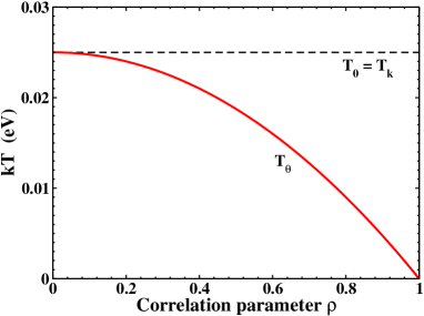
Figure 1: (color online) Kinetic ($kT_{k}$ = $kT_{0}$) and thermodynamic ($kT_{\theta}$) thermal energy (in eV) for different values of the correlation coefficient $\rho$. The reservoir temperature is assumed to be 300 K, for $kT_{0}$ = 0.025 eV.

This allows to calculate both Fisher information $J(x)$ = $\sigma_{x}^{-2}$ and $J(x,y)$:

$$J(x,y) = \beta\left\langle\frac{\partial^{2}\mathcal{\tilde{E}}}{\partial x^{2}}\right\rangle=\frac{1}{(1-\rho^{2})\sigma^{2}_{x}},$$ (21)

which leads to $\gamma$ equals to:

$$\gamma = \frac{2A(1-\rho^{2})\sigma^{2}_{x}}{kT_{0}}=(1-\rho^{2})=\frac{T_{\theta}}{T_{0}}.$$ (22)

The thermodynamic temperature is reduced respect to $T_{0}$ by increasing the correlation (see figure 1). The average energy on the contrary is not affected by the correlation and then kinetic temperature $T_{k}$ = $T_{0}$. Because the heat and work exchanged depend on different temperatures (eq. 1), in this particular case we obtain that $\Delta Q$ = -$\Delta W$ $\propto$ ($T_{0}-T_{\theta}$). This means, as should be, that in equilibrium condition, even when information is acquired, the total energy flux $\Delta Q$ + $\Delta W$ is zero. However, we observe that the single fluxes are not zero, in particular the system absorbs heat ($\Delta Q$ $>$ 0) and makes mechanical work to the reservoir ($\Delta W$ $<$ 0).

The explanation of the example is the following. Using the information about the momentum of the particle, the reservoir can extract mechanical work from it. For example using a small mill, that can be rotated by the particle. In equilibrium conditions the impacts between particle and mill do not produce net mechanical work, because there are equal impacts in one direction and in the opposite. However, if the reservoir can estimate the dynamical state of the particle with more accuracy, then can use the mill to extract work when the particle moves in one direction and block the mill when the particle comes from the opposite direction. The impact transfers energy from the particle to the reservoir in form of a net mechanical work. The particle cools down because its average energy is reduced by the series of impacts. However, the particle is also in thermal contact with the reservoir, if the temperature of the particle gets lower than the reservoir, a heat transfer occurs increasing again the average energy of the particle.

So, even if the net flux of energy is zero, the entropy flux is not. The system absorbs energy with high entropy (heat) and gives back to the reservoir energy with a lower entropy (work). This is consistent with the fact that, thanks to the information due to correlation with the microstate, the system behaves with respect to the reservoir more and more like a deterministic system. Its internal average energy can be exploited to make work. In fact, in the limit of perfect correlation $T_{\theta}$ = 0 and $F$ = $\bar{E}$.

It is important to stress that this is not implying any violation of the second principle of thermodynamics. The reduction of entropy performed in the system occurs only thanks to the information obtained. The harvesting and elaboration of this information requires work made at the expense of the reservoir. The variation of entropy due to this elaboration more than compensate the local reduction in entropy in the system. Then the total entropy variation, system plus reservoir, is still non negative.

In this work a generalization of the free energy potential has been presented. This formalism makes use of informational theory concepts in order to extend the thermodynamic theory to systems which share information with the reservoir or are in steady state non-equilibrium. The core point is the concept of mutual information and conditional Fisher information, which allow to generalize both entropy and thermodynamic temperature definitions, respectively. A simple model, describing a single free particle, has been discussed showing the effect of shared information over the thermodynamics between system and reservoir. Increasing the correlation between measure and microstate allows to consider the system more and more as deterministic. Then its internal energy can be entirely converted into work.

References

- (1) G. E. Crooks, Excursions in Statistical Dynamics, PhD Thesis, University of California at Berkley, 1999.
- (2) C. Jarzynski, Non-equilibrium equality for free energy differences, Phys. Rev. Lett., vol. 78, 2690 (1997).
- (3) D. A. Sivak, G. E. Crooks, Near-equilibrium measurements of nonequilibrium free energy, Phys. Rev. Lett., vol. 108, 150601 (2012).
- (4) E. Boksenbojm, B. Wynants and C. Jarzynski, Nonequilibrium thermodynamics at the microscale: work relations and the second law, arXiv:1002.1230v1, (2010).
- (5) W. Muschik, Aspects of non-equilibrium thermodynamics, Singapore (World Scientific), (1990).
- (6) G. E. Crooks, Entropy production fluctuation theorem and the non-equilibrium work relation for free energy differences, Phys. Rev. E, vol. 60, 2721 (1999).
- (7) G. E. Crooks, Path-ensemble averages in system driven far from equilibrium, Phys. Rev. E, vol. 61, 2361 (2000).
- (8) D. N. Zubarev et al., Statistical Mechanics of Nonequilibrium Processes, (Berlin: Akademie), (1996).
- (9) R. Luzzi et al, Statistical Foundations of Irreversible Thermodynamics, (Leipzig: Teubner), (2001).
- (10) Y. Dubi, M. Di Ventra, Colloquium: Heat flow and thermoelectricity in atomic and molecular junctions, Rev. Mod. Phys., vol. 83, 131 (2011).
- (11) J. C. Vasquez and D. Jou, Temperature in non-equilibrium states: a review of open problems and current proposals, Rep. Prog. Phys., vol. 66, 1937 (2004).
- (12) T. Sagawa and M. Ueda, Phys. Rev. E, 85, 021104 (2012).
- (13) T. Sagawa and M. Ueda, Phys. Rev. Lett., 109, 180602 (2012).
- (14) A. Gagliardi and A. Di Carlo,Phys. A, vol. 391, 6337 (2012).
- (15) K. Huang, ”Statistical Mechanics (2nd ed.)”, Wyley (1987).
- (16) K. R. Narayanan and A. R. Sanistrava,Phys. Rev. E, vol. 85, 031151 (2012).
- (17) T. M. Cover and J. A. Thomas, ”Elements of information theory”, Wyley (2006).
- (18) E. T. Jaynes, Information theory and statistical mechanics, Phys. Rev. A, vol. 106, 620 (1957).
- (19) E. T. Jaynes, Information theory and statistical mechanics - II, Phys. Rev. A, vol. 108, 171 (1957).
- (20) L. Brillouin, Science and Information Theory, Mineola, N.Y.: Dover, 2004.
- (21) N. Merhav, Statistical Physics and Information theory, Foundation and Trends in Communication and Information Theory, vol. 6, 1-212 (2009).
- (22) G. B. Bagci, The physical meaning of Renyi relative entropies, arXiv:cond-mat/0703008v1, (2007).
- (23) R. Landauer, Irreversibility and Heat Generation in the Computing Process, IBM J. Res. Develop., Vol. 5, No. 3, 183(1961).
- (24) J. Horowitz and C. Jarzynski, An illustrative example of the relationship between dissipation and relative entropy, arXiv:0901.0576v1, (2009).
- (25) S. Kullback, Information theory and statistics, Dover (1978).
- (26) F. Pennini, A.R. Plastino, A. Plastino, Phys. A, vol. 258, 446 (1998).
- (27) J. Shao, ”Mathematical Statistics”, New York: Springer (1998).
- (28) D. Guo, S. Shamai and S. Verdu, IEEE Trans. Information Theory, vol. 51, 1261 (2005).
- (29) S. Park, E. Serpedin and K. Qaraqe, arXiv:1202.0015v4 (2012).
- (30) T. Sagawa and M. Ueda, Phys. Rev. Lett., 104, 090602 (2010).
- (31) The PD of the components of are assumed to be independent and identically normal distributed with 0 mean value and unitary variance.