Second-order Born approximation for the scattering phase shifts: Application to the Friedel sum rule

Abstract

Screening effects are important to understand various aspects of ion-solid interactions and, in particular, play a crucial role in the stopping of ions in solids. In this paper the phase shifts and scattering amplitudes for the quantum-mechanical elastic scattering within up to the second-order Born (B2) approximation are revisited for an arbitrary spherically-symmetric electron-ion interaction potential. The B2 phase shifts and scattering amplitudes are then used to derive the Friedel sum rule (FSR) involving the second-order Born corrections. This results in a simple equation for the B2 perturbative screening parameter of an impurity ion immersed in a fully degenerate electron gas which, as expected, turns out to depend on the ion atomic number $Z_{1}$ unlike the first-order Born (B1) screening parameter reported earlier by some authors. Furthermore, our analytical results for the Yukawa, hydrogenic, Hulthén, and Mensing potentials are compared, for both positive and negative ions and a wide range of one-electron radii, to the exact screening parameters calculated self-consistently by imposing the FSR requirement. It is shown that the B2 screening parameters agree excellently with the exact values at large and moderate densities of the degenerate electron gas, while at lower densities they progressively deviate from the exact numerical solutions but are nevertheless more accurate than the prediction of the B1 approximation. In addition, a simple Padé approximant to the Born series has been developed that improves the performance of the perturbative FSR for any negative ion as well as for $Z_{1}=+1$.

1 Introduction

The problem of ion interactions in condensed matter continues to be the subject of intense experimental and theoretical research. These interactions are relevant to understand, among others, the behavior of static impurities in metals, such as the resistivity of impurities and metallic solutions [1], or the stopping of ions in solids [2]. The screening of the intruder ion in the host medium plays a key role in these phenomena.

A number of approaches, both perturbative and non-perturbative, have been devised over the years to describe the basic processes of ion-solid interactions. In particular, following the pioneering works of Lindhard [3], and Lindhard and Winther [4], many calculations have been done within the framework of linear-response theory (see, e.g., [5, 6, 7, 8, 9, 10, 11, 12, 13]), which enables a unified description of dynamical screening, plasmon excitation, and creation of electron-hole pairs. Most of these calculations are based on the dielectric function in the random-phase approximation (RPA) which is valid in the weak-coupling (i.e., high-density) limit of a degenerate electron gas (DEG). The main shortcoming of linear-response theory is observed in the low-velocity limit since the interaction effects become too strong to be properly accounted for by perturbative approximations [14].

Non-perturbative (i.e., non-linear) methods also provide a reasonable description of ion-solid interactions. For instance, the kinetic theory [15, 16] involves the transport cross section for dynamically-screened interactions including quantum effects in the whole velocity range. However, though non-perturbative in the ion-solid coupling, the formalism does not include contributions from collective (plasmon) excitations to the stopping power, which are important in the high-velocity regime when the interaction potential becomes highly anisotropic. These quantum-mechanical models were initially proposed for the case of slow ions. In [17] a transport cross section approach based on the partial-wave expansion was introduced to calculate the stopping power of positive ions in channeling conditions, explaining qualitatively the observed oscillatory behavior of this quantity with the ion atomic number $Z_{1}$ (“$Z_{1}$ oscillations”). A more rigorous many-body representation of the non-linear screening and stopping processes in a homogeneous DEG was subsequently given in [18, 19, 20, 21] working within density-functional theory. A computationally convenient simplification is achieved if the numerical density-functional-theory potential is substituted by an analytical electron-ion interaction potential with a free parameter that is adjusted self-consistently requiring that the scattering phase shifts satisfy the Friedel sum rule [22, 23, 24, 25, 26, 27]. It is possible to introduce in the analytical potential more parameters, which are adjusted demanding the fulfillment of additional constraints like Kato’s cusp condition in the self-consistent procedure [28, 29]. The aforementioned non-linear approaches can be adapted immediately to deal with inhomogeneous DEGs having recourse to the local-plasma approximation; this allows a realistic description of the screening and energy loss of low-energy ions in the spatially-varying electron densities encountered in solids [30, 31, 32, 29].

The problem of extending the quantum treatments to finite velocities has been addressed more recently in the context of density-functional theory [33] and by means of model potentials with and without the Born approximation [34, 35, 36, 37, 38]. For instance, extensions of the Friedel sum rule to finite velocities have been formulated either making use of the first-order Born (B1) approximation [34] or including all orders in the interaction strength [35]. In these formalisms the dynamical potential is replaced by a spherically symmetric one which facilitates the application of the conventional partial-wave analysis of one-electron scattering phase shifts. In the present article we too rely on this assumption.

This work concerns itself with the perturbative treatment of screening effects in the case of static or slow ions in a DEG. The B1 approximation yields a screening parameter that is independent of the ion atomic number $Z_{1}$ and hence is the same for slow particles and antiparticles [20]. This situation is somewhat unsatisfactory in analyzing the available experimental data on proton and antiproton energy losses in various solids [39, 40, 41]. Recently, using the Friedel sum rule the screening lengths within the second-order Born (B2) approximation have been deduced in [38] for the Yukawa and Mensing interaction potentials. These B2 screening lengths pertaining to protons and antiprotons agree satisfactorily with the exact numerical solutions at electron densities typical of metals. However, in [38] only some simplified expressions of the screening lengths were studied and further investigation on this topic seemed desirable. To carry out this idea we evaluate the scattering amplitude and phase shifts within the B2 approximation and for an arbitrary interaction potential, which allows us to formulate explicitly the Friedel sum rule at the same level of the B2 approximation.

The scattering phase shifts are derived within the B2 approximation in Section 2 for an arbitrary spherically-symmetric interaction potential. In Section 3 we employ these results to derive the second-order Friedel sum rule. Based on this sum rule we have developed a simple but general equation that determines the screening length, within the B2 approximation, for arbitrary screened potentials. Moreover, this equation has been specified for the Yukawa, hydrogenic, Hulthén, and Mensing potentials. The perturbative results for these potentials are compared, in Section 4, with the corresponding exact solutions calculated from the Friedel sum rule in a wide range of DEG densities and for several charges of the impurity ion. Finally, the Padé approximant for the obtained Born series in the Friedel sum rule has also been examined. Some details of the analytical calculations are included in Appendices A, B, and C.

2 First- and second-order phase shifts and scattering amplitudes

In this section we deduce, within the Born approximation, the B1 and B2 scattering phase shifts using the systematic perturbative expansion of the exact scattering amplitude and the exact electronic wave function at the final state (after scattering). Although the B1 and B2 phase shifts are well known (see, e.g., [42]), we suggest an alternative derivation of these quantities which is more suitable for the evaluation of the perturbative screening parameters in Section 3. The starting point is the exact relation between the scattering amplitude $f(k,\theta)$ for the elastic scattering and the phase shifts $\delta_{\ell}(k)$ which is given by [43]

$$f(k,\theta)=\frac{1}{2\mathrm{i}k}\,\sum_{\ell=0}^{\infty}(2\ell+1)\left(\mathrm{e}^{2\mathrm{i}\delta_{\ell}}-1\right)P_{\ell}(\cos\theta).$$ (1)

Here $k$ is the electron wave number, $\theta$ is the scattering angle, and $P_{\ell}$ are the Legendre polynomials. Within the Born approximation we assume that the $n$-th order phase shifts are determined by $\delta_{\ell,\mathrm{B}n}\sim B^{n}$ with $n=1,2,\ldots$, where $B$ is the Born “smallness parameter” which should be precisely determined for each interaction potential. It is clear that $B\sim V(r)$, where $V(r)$ is the isotropic (i.e., spherically symmetric) interaction potential of the colliding particles. In this paper we restrict ourselves to the B2 approximation and look for the phase shifts in a perturbative manner $\delta_{\ell}=\delta_{\ell,\mathrm{B}1}+\delta_{\ell,\mathrm{B}2}$, where $\delta_{\ell,\mathrm{B}1}$ and $\delta_{\ell,\mathrm{B}2}$ are the first- and second-order phase shifts, respectively. Analogously, the scattering amplitude in Eq. (1) can be written as $f=f_{\mathrm{B}1}+f_{\mathrm{B}2}$, where $f_{\mathrm{B}1}$ and $f_{\mathrm{B}2}$ are the first- and second-order amplitudes, respectively. Next, using the perturbative expansion of the phase shift we rewrite the exponential factor in Eq. (1) in the form $(\mathrm{e}^{2\mathrm{i}\delta_{\ell}}-1)/2\mathrm{i}\simeq\delta_{\ell}+\mathrm{i}\delta_{\ell}^{2}\simeq\delta_{\ell,\mathrm{B}1}+\delta_{\ell,\mathrm{B}2}+\mathrm{i}\delta_{\ell,\mathrm{B}1}^{2}$. Then, keeping only terms up to the second order we have

$$f_{\mathrm{B}1}(k,\theta) = \frac{1}{k}\,\sum_{\ell=0}^{\infty}(2\ell+1)\,\delta_{\ell,\mathrm{B}1}\,P_{\ell}(\cos\theta),$$ (2)

$$f_{\mathrm{B}2}(k,\theta) = \frac{1}{k}\,\sum_{\ell=0}^{\infty}(2\ell+1)\left(\delta_{\ell,\mathrm{B}2}+\mathrm{i}\delta_{\ell,\mathrm{B}1}^{2}\right)P_{\ell}(\cos\theta).$$ (3)

Note that the imaginary part of $f_{\mathrm{B}1}(k,\theta)$ vanishes while the imaginary part of the B2 scattering amplitude at $\theta=0$ (forward scattering) satisfies the optical theorem $\mathop{\mathrm{Im}}\nolimits\big{[}f_{\mathrm{B}2}(k,0)\big{]}=(k/4\pi)\,\sigma_{\mathrm{tot,B}1}(k)$ [42] within the B2 approximation, where $\sigma_{\mathrm{tot,B}1}(k)$ is the B1 total elastic cross section.

To determine the first- and second-order phase shifts, Eqs. (2) and (3) should be compared with the corresponding scattering amplitudes extracted from the systematic perturbative expansion of the exact electronic wave function at the final state (see, e.g., [43]). This procedure is straightforward and leads to

$$f_{\mathrm{B}1}(k,\theta) = -\frac{m_{\mathrm{e}}}{2\pi\hbar^{2}}\int V(r)\,\varphi_{\mathbf{k}_{f}}^{\ast}(\mathbf{r})\,\varphi_{\mathbf{k}_{i}}(\mathbf{r})\,\mathrm{d}\mathbf{r},$$ (4)

$$f_{\mathrm{B}2}(k,\theta) = \left(\frac{m_{\mathrm{e}}}{2\pi\hbar^{2}}\right)^{2}\int\!\int\frac{\mathrm{e}^{\mathrm{i}k\left|\mathbf{r}-\mathbf{r}^{\prime}\right|}}{\left|\mathbf{r}-\mathbf{r}^{\prime}\right|}\,V(r)\,V(r^{\prime})\,\varphi_{\mathbf{k}_{f}}^{\ast}(\mathbf{r})\,\varphi_{\mathbf{k}_{i}}(\mathbf{r}^{\prime})\,\mathrm{d}\mathbf{r}\,\mathrm{d}\mathbf{r}^{\prime},$$ (5)

where $\mathbf{k}_{i}$ and $\mathbf{k}_{f}$ are the initial and final wave vectors of the electron, respectively. Let us recall that we assume here an elastic scattering process with momentum conservation, i.e., $k_{f}=k_{i}=k$. Also $\varphi_{\mathbf{k}}(\mathbf{r})=\mathrm{e}^{\mathrm{i}\mathbf{k}\cdot\mathbf{r}}$ is the unperturbed electronic wave function corresponding to the wave vector $\mathbf{k}$. Thus, from Eqs. (4) and (5) one has

$$f_{\mathrm{B}1}(k,\theta) = -\frac{m_{\mathrm{e}}}{2\pi\hbar^{2}}\,\widetilde{V}(q),$$ (6)

$$f_{\mathrm{B}2}(k,\theta) = \left(\frac{m_{\mathrm{e}}}{2\pi\hbar^{2}}\right)^{2}\int\!\int\frac{\mathrm{e}^{\mathrm{i}k\left|\mathbf{r}-\mathbf{r}^{\prime}\right|}}{\left|\mathbf{r}-\mathbf{r}^{\prime}\right|}\,V(r)\,V(r^{\prime})\,\mathrm{e}^{-\mathrm{i}\mathbf{k}_{f}\cdot\mathbf{r}}\,\mathrm{e}^{\mathrm{i}\mathbf{k}_{i}\cdot\mathbf{r}^{\prime}}\,\mathrm{d}\mathbf{r}\,\mathrm{d}\mathbf{r}^{\prime}.$$ (7)

Here $\mathbf{q}=\mathbf{k}_{f}-\mathbf{k}_{i}$ is the momentum transfer in the elastic collision with $q=2k\sin(\theta/2)$ and $\widetilde{V}(q)$ is the Fourier transform of the interaction potential. Note that $\widetilde{V}(q)$ is spherically symmetric in momentum space and is given by

$$\widetilde{V}(q)=\int_{0}^{\infty}V(r)\,j_{0}(qr)\,4\pi r^{2}\,\mathrm{d}r,$$ (8)

where $j_{\ell}(z)$ are the spherical Bessel functions of the first kind and order $\ell$ with $j_{0}(z)=\sin z/z$ [44, 45].

Equation (6) can be developed further if in Eq. (8) we replace $j_{0}(qr)$ with (see Eq. (10.1.45) in [44])

$$j_{0}\big{(}2kr\sin(\theta/2)\big{)}=\sum_{\ell=0}^{\infty}(2\ell+1)\,j_{\ell}^{2}(kr)\,P_{\ell}(\cos\theta).$$ (9)

Comparing the resulting expression for $f_{\mathrm{B}1}(k,\theta)$ with Eq. (2) we conclude that (see, e.g., [42])

$$\delta_{\ell,\mathrm{B}1}(k)=-\frac{2m_{\mathrm{e}}k}{\hbar^{2}}\,\int_{0}^{\infty}V(r)\,j_{\ell}^{2}(kr)\,r^{2}\,\mathrm{d}r.$$ (10)

On the other hand, in Eq. (7) we may expand $\mathrm{e}^{\mathrm{i}k|\mathbf{r}-\mathbf{r}^{\prime}|}/|\mathbf{r}-\mathbf{r}^{\prime}|$ with the help of Eq. (B.43) in [42] and use the Rayleigh expansion of the plane wave over spherical harmonics to deal with $\mathrm{e}^{-\mathrm{i}\mathbf{k}_{f}\cdot\mathbf{r}}$ and $\mathrm{e}^{\mathrm{i}\mathbf{k}_{i}\cdot\mathbf{r}^{\prime}}$. After some algebraic manipulations that involve the orthonormality relation and the addition theorem of spherical harmonics [45, 44] one obtains

$$f_{\mathrm{B}2}(k,\theta) = \mathrm{i}k\left(\frac{2m_{\mathrm{e}}}{\hbar^{2}}\right)^{2}\sum_{\ell=0}^{\infty}(2\ell+1)\,P_{\ell}(\cos\theta)$$ (11)

$$\mbox{}\times\int_{0}^{\infty}V(r)\,j_{\ell}(kr)\,r^{2}\,\mathrm{d}r$$

$$\mbox{}\times\int_{0}^{\infty}V(r^{\prime})\,j_{\ell}(kr_{<})\,h_{\ell}^{(1)}(kr_{>})\,j_{\ell}(kr^{\prime})\,r^{\prime 2}\,\mathrm{d}r^{\prime}.$$

Here $h_{\ell}^{(1)}(z)=j_{\ell}(z)+\mathrm{i}n_{\ell}(z)$ are the spherical Hankel functions of the first kind, $n_{\ell}(z)$ are the spherical Bessel functions of the second kind [44], $r_{<}=\min\{r,r^{\prime}\}$, and $r_{>}=\max\{r,r^{\prime}\}$. Comparing now the real parts of Eqs. (11) and (3) we finally get (see, e.g., [42])

$$\delta_{\ell,\mathrm{B}2}(k) = -\left(\frac{2m_{\mathrm{e}}k}{\hbar^{2}}\right)^{2}\int_{0}^{\infty}V(r)\,j_{\ell}(kr)\,r^{2}\,\mathrm{d}r$$ (12)

$$\mbox{}\times\int_{0}^{\infty}V(r^{\prime})\,j_{\ell}(kr_{<})\,n_{\ell}(kr_{>})\,j_{\ell}(kr^{\prime})\,r^{\prime 2}\,\mathrm{d}r^{\prime}.$$

It is easy to verify that the imaginary parts of Eqs. (11) and (3) are identical because of the relation (10) for the B1 phase shifts. Equations (10) and (12) thus represent the first- and second-order phase shifts, respectively. As expected, they are proportional to $\sim V(r)$ and $\sim V^{2}(r)$, respectively. It should be emphasized that Eqs. (10) and (12) are valid when $B<1$, which in particular is satisfied at high velocities (large $k$) or in the case of a weak interaction potential. In addition, the validity of the Born approximation requires that $\delta_{\ell,\mathrm{B}2}<\delta_{\ell,\mathrm{B}1}$, which in general is fulfilled at high velocities. At small velocities (small $k$) using the asymptotic behavior of the spherical Bessel functions [44] it is not difficult to show that the B1 and B2 phase shifts of Eqs. (10) and (12) behave as $\delta_{\ell}\sim(k\lambda)^{2\ell+1}$, where $\lambda$ is the characteristic range of the interaction potential (see, e.g., [42, 43]). In this case $\delta_{\ell,\mathrm{B}2}/\delta_{\ell,\mathrm{B}1}\simeq\overline{V}(m_{\mathrm{e}}\lambda^{2}/\hbar^{2})[2^{2\ell}(2\ell+1)]^{-1}$ is independent of $k$, but depends on the average interaction potential $\overline{V}$ (potential at the distance $\lambda$). Therefore, at $\overline{V}<\hbar^{2}/m_{\mathrm{e}}\lambda^{2}$ systematically $\delta_{\ell,\mathrm{B}2}<\delta_{\ell,\mathrm{B}1}$ for all $\ell$, while at $\overline{V}>\hbar^{2}/m_{\mathrm{e}}\lambda^{2}$ the requirement of the Born approximation is satisfied at large angular momentum $\ell$.

We would like to close this section with the following remark. An alternative, shorter way to derive the first- and second-order phase shifts within the Born approximation starts from the Calogero equation [46]

$$\frac{\mathrm{d}\Delta_{\ell}(r)}{\mathrm{d}r} = -\frac{2m_{\mathrm{e}}k}{\hbar^{2}}\,r^{2}\,V(r)$$ (13)

$$\mbox{}\times\Big{[}j_{\ell}(kr)\,\cos\Delta_{\ell}(r)-n_{\ell}(kr)\,\sin\Delta_{\ell}(r)\Big{]}^{2}$$

for the generalized (coordinate dependent) phase shifts $\Delta_{\ell}(r)$. The scattering phase shifts $\delta_{\ell}$ are then deduced according to the limit $\delta_{\ell}=\Delta_{\ell}(r)|_{r\to\infty}$. Let us note that this relation along with Eq. (13) determines the absolute phase shifts of the scattering problem while most of the existing numerical methods deliver, instead, relative phase shifts by solving the radial Schrödinger equation. However, absolute $\delta_{\ell}$ are needed for certain applications like, for example, in the Friedel sum rule (see Eq. (17) below).

Let us look for the solution of Eq. (13) in a perturbative manner. Within the B1 and B2 approximations the generalized phase shifts are denoted as $\Delta_{\ell,\mathrm{B}1}(r)$ and $\Delta_{\ell,\mathrm{B}2}(r)$, respectively, and from Eq. (13) it is straightforward to see that

$$\Delta_{\ell,\mathrm{B}1}(r)=-\frac{2m_{\mathrm{e}}k}{\hbar^{2}}\,\int_{0}^{r}V(r^{\prime})\,j_{\ell}^{2}(kr^{\prime})\,r^{\prime 2}\,\mathrm{d}r^{\prime}$$ (14)

and

$$\Delta_{\ell,\mathrm{B}2}(r) = \frac{4m_{\mathrm{e}}k}{\hbar^{2}}\int_{0}^{r}V(r^{\prime})\,j_{\ell}(kr^{\prime})\,n_{\ell}(kr^{\prime})\,\Delta_{\ell,\mathrm{B}1}(r^{\prime})r^{\prime 2}\,\mathrm{d}r^{\prime}$$ (15)

$$= -2\left(\frac{2m_{\mathrm{e}}k}{\hbar^{2}}\right)^{2}\int_{0}^{r}V(r^{\prime})j_{\ell}(kr^{\prime})\,n_{\ell}(kr^{\prime})\,r^{\prime 2}\,\mathrm{d}r^{\prime}$$

$$\mbox{}\times\int_{0}^{r^{\prime}}V(r^{\prime\prime})\,j_{\ell}^{2}(kr^{\prime\prime})\,r^{\prime\prime 2}\,\mathrm{d}r^{\prime\prime}.$$

Taking the limit $r\to\infty$ in (14) and (15) we recover Eq. (10) for the first-order phase shifts $\delta_{\ell,\mathrm{B}1}$ while Eq. (15) yields

$$\delta_{\ell,\mathrm{B}2} = -2\left(\frac{2m_{\mathrm{e}}k}{\hbar^{2}}\right)^{2}\int_{0}^{\infty}V(r)\,j_{\ell}(kr)\,n_{\ell}(kr)\,r^{2}\,\mathrm{d}r$$ (16)

$$\mbox{}\times\int_{0}^{r}V(r^{\prime})\,j_{\ell}^{2}(kr^{\prime})\,r^{\prime 2}\,\mathrm{d}r^{\prime}.$$

To prove the identity of Eqs. (12) and (16) we write the latter in an equivalent form by changing the orders of the integrations. Then, taking half of the sum of the obtained expression and Eq. (16) we arrive at Eq. (12) for the second-order phase shifts $\delta_{\ell,\mathrm{B}2}$ derived directly from the systematic perturbative expansion of the exact scattering amplitude.

3 Application to the Friedel sum rule

With the perturbative formalism presented in Section 2, we now take up the main topic of this paper, namely to study the Friedel sum rule (FSR) for a point-like static (or slow) ion in a DEG of density $n_{\mathrm{e}}$ within up to the B2 approximation. The FSR is very useful to adjust in a self-consistent way the electron-ion interaction potential and the related screening length. The Born approximation has been used before in conjunction with the FSR, but only within the first order [20, 34, 35]. This is somewhat unsatisfactory since the resulting (first-order) screening length is independent of $Z_{1}$ and is therefore identical for particles and their antiparticles. Going beyond the B1 approximation, and considering the B2 approximation, allows more physical insight and furnishes useful numerical estimates of the influence of the ion charge on the screening length in a DEG. The problem is closely related to the formulation of the theory of the higher-order stopping power involving the Barkas correction (see, e.g., [6] and references therein) which is $\sim Z_{1}^{3}$ and is not symmetric with respect to the sign of $Z_{1}$.

Let us consider the usual treatment of the FSR for static ions [47, 48]. It may be shown that each scattered electron contributes to the accumulation of screening charge by an amount that, in a partial-wave expansion, is given by the derivative of the phase shift in the form $\Delta Q_{\ell}=(1/\pi)(\mathrm{d}\delta_{\ell}/\mathrm{d}k)$. The FSR embodies the condition of overall charge neutrality, expected for a metallic environment, as a consequence of the screening by all the electron states within the Fermi sphere. In general form the rule may be expressed as [47, 48]

$$Z_{1}=\frac{2}{\pi}\,\sum_{\ell=0}^{\infty}(2\ell+1)\,\delta_{\ell}(k_{\mathrm{F}}),$$ (17)

where $k_{\mathrm{F}}=(9\pi/4)^{1/3}(a_{0}r_{\mathrm{s}})^{-1}$ is the Fermi wave vector. Here $a_{0}$ is the Bohr radius, and the (dimensionless) one-electron radius (or Wigner–Seitz density parameter) $r_{\mathrm{s}}$ is defined through the relation $\frac{4}{3}\pi(r_{\mathrm{s}}a_{0})^{3}=n_{\mathrm{e}}^{-1}$. In this circumstance of static screening the integral over the electron wave vectors $k$ extends over a Fermi sphere of radius $k_{\mathrm{F}}$ (cf. [33, 35]). Without loss of generality we have not included explicitly in Eq. (17) the contribution of the bound electrons in which case the charge number $Z_{1}$ should be simply replaced by $Z_{1}-N_{\mathrm{b}}$, being $N_{\mathrm{b}}$ the number of bound electrons [47, 48].

Within the B2 approximation the FSR (17) reads

$$Z_{1}=\frac{2}{\pi}\,\sum_{\ell=0}^{\infty}(2\ell+1)\,\big{[}\delta_{\ell,\mathrm{B}1}(k_{\mathrm{F}})+\delta_{\ell,\mathrm{B}2}(k_{\mathrm{F}})\big{]},$$ (18)

The right-hand side of the relation (18) can be evaluated by substituting Eqs. (10) and (12) for the first- and second-order phase shifts, respectively. However, the simplest way is to express the right-hand side of Eq. (18) through the scattering amplitudes $f_{\mathrm{B}1}(k,0)$ and $f_{\mathrm{B}2}(k,0)$ for forward scattering (i.e., at $\theta=0$). From Eqs. (2) and (3) one obtains

$$\sum_{\ell=0}^{\infty}(2\ell+1)\left[\delta_{\ell,\mathrm{B}1}(k)+\delta_{\ell,\mathrm{B}2}(k)\right]=k\,\Big{\{}f_{\mathrm{B}1}(k,0)+\mathop{\mathrm{Re}}\nolimits\big{[}f_{\mathrm{B}2}(k,0)\big{]}\Big{\}}.$$ (19)

The forward-scattering amplitudes $f_{\mathrm{B}1}(k,0)$ and $f_{\mathrm{B}2}(k,0)$ are easily evaluated from Eqs. (6) and (7),

$$f_{\mathrm{B}1}(k,0) = -\frac{m_{\mathrm{e}}}{2\pi\hbar^{2}}\widetilde{V}(0),$$ (20)

$$f_{\mathrm{B}2}(k,0) = \left(\frac{m_{\mathrm{e}}}{2\pi\hbar^{2}}\right)^{2}\int\!\int\frac{\mathrm{e}^{\mathrm{i}k\left|\mathbf{r}-\mathbf{r}^{\prime}\right|}}{\left|\mathbf{r}-\mathbf{r}^{\prime}\right|}\,V(r)\,V(r^{\prime})\,\mathrm{e}^{\mathrm{i}k\hat{\mathbf{n}}\cdot(\mathbf{r}^{\prime}-\mathbf{r})}\,\mathrm{d}\mathbf{r}\,\mathrm{d}\mathbf{r}^{\prime}.$$ (21)

In Eq. (21) we have made $\mathbf{k}_{f}=\mathbf{k}_{i}=k\hat{\mathbf{n}}$, being $\hat{\mathbf{n}}$ a unit vector, and $\widetilde{V}(0)$ is the Fourier transform of the interaction potential at $q=0$. Thus, inserting Eqs. (20) and (21) into (19) the FSR (18) within up to the B2 approximation is written as

$$Z_{1} = \frac{2}{\pi}\,k_{\mathrm{F}}\,\Big{\{}f_{\mathrm{B}1}(k_{\mathrm{F}},0)+\mathop{\mathrm{Re}}\nolimits\big{[}f_{\mathrm{B}2}(k_{\mathrm{F}},0)\big{]}\Big{\}}$$ (22)

$$= -\frac{m_{\mathrm{e}}k_{\mathrm{F}}}{\pi^{2}\hbar^{2}}\left[\widetilde{V}(0)+\frac{8\pi m_{\mathrm{e}}k_{\mathrm{F}}}{\hbar^{2}}\,\Sigma(k_{\mathrm{F}})\right]$$ (23)

with

$$\Sigma(k)=-\frac{1}{4(2\pi)^{2}k}\,\mathop{\mathrm{Re}}\nolimits\left[\int\!\int\frac{\mathrm{e}^{\mathrm{i}kr^{\prime}}}{r^{\prime}}\,V(r)\,V(|\mathbf{r}^{\prime}+\mathbf{r}|)\,\mathrm{e}^{\mathrm{i}k\hat{\mathbf{n}}\cdot\mathbf{r}^{\prime}}\,\mathrm{d}\mathbf{r}\,\mathrm{d}\mathbf{r}^{\prime}\right].$$ (24)

In the last step of deriving Eq. (24) we have changed the integration variable $\mathbf{r}^{\prime}$ according to $\mathbf{r}^{\prime}\to\mathbf{r}^{\prime}+\mathbf{r}$. Using now the Fourier transform $\widetilde{V}(\mathbf{q})$ of the interaction potential, the function $\Sigma(k)$ may be represented as

$$\Sigma(k)=-\frac{1}{2(2\pi)^{4}k}\,\int\frac{|\widetilde{V}(\boldsymbol{\kappa})|^{2}\,\mathrm{d}\boldsymbol{\kappa}}{(\boldsymbol{\kappa}+\mathbf{k})^{2}-k^{2}},$$ (25)

where we have used the property $\widetilde{V}(-\mathbf{q})=\widetilde{V}^{\ast}(\mathbf{q})$. For a spherically-symmetric interaction potential the Fourier transform is also spherically symmetric, $\widetilde{V}(\mathbf{q})=\widetilde{V}(q)$, and in addition it is a real quantity. Then, after performing the angular integration in Eq. (25) we finally arrive at

$$\Sigma(k)=-\frac{1}{4(2\pi)^{3}k^{2}}\,\int_{0}^{\infty}\widetilde{V}^{2}(\kappa)\,\ln\left|\frac{\kappa+2k}{\kappa-2k}\right|\,\kappa\,\mathrm{d}\kappa.$$ (26)

Equation (23) is the main result of the present article. The first and second terms in this expression are linear ($\sim Z_{1}$) and quadratic ($\sim Z_{1}^{2}$) with respect to the interaction potential representing, respectively, the first- and second-order Born contributions to the FSR. While the first term in Eq. (23) has been derived and studied previously [20, 34, 35] the second one is a new result that may be viewed as a counterpart of the Barkas correction to the FSR. In general, Eq. (23) is a transcendental equation that serves to determine the screening length $\lambda\equiv 1/\alpha$, where $\alpha$ is the corresponding screening parameter, of the interaction potential involved in $\widetilde{V}(0)$ and $\Sigma(k_{\mathrm{F}})$.

In what follows we apply the FSR in the B2 approximation, Eq. (23), to the very important case of screened potentials of the form

$$V(r)=-\frac{Z_{1}e^{2}}{r}\,\Phi(\alpha r),$$ (27)

where $\Phi(x)$ is the screening function. Then

$$\widetilde{V}(q)=-(4\pi Z_{1}e^{2}/\alpha^{2})\,\widetilde{\mathcal{V}}(q/\alpha),$$ (28)

where

$$\widetilde{\mathcal{V}}(x)=\int_{0}^{\infty}\Phi(y)\,j_{0}(xy)\,y\,\mathrm{d}y$$ (29)

is the dimensionless Fourier transform of the interaction potential. In terms of $\widetilde{\mathcal{V}}(x)$ we have $\widetilde{V}(0)=-(4\pi Z_{1}e^{2}/\alpha^{2})\,\gamma$ with

$$\gamma=\widetilde{\mathcal{V}}(0)=\int_{0}^{\infty}\Phi(x)\,x\,\mathrm{d}x$$ (30)

and $\Sigma(k_{\mathrm{F}})=-(Z^{2}_{1}e^{4}/4k_{\mathrm{F}}^{2}\alpha^{2})\,g(u)$ with $u=2k_{\mathrm{F}}/\alpha$ and

$$g(u)=\frac{2}{\pi}\,\int_{0}^{\infty}\widetilde{\mathcal{V}}^{2}(x)\,\ln\left|\frac{x+u}{x-u}\right|\,x\,\mathrm{d}x.$$ (31)

Inserting $\widetilde{\mathcal{V}}(x)$, Eq. (29), into (31) and using expression (57) in A we may, alternatively, write $g(u)$ in coordinate space via the relation

$$g(u)=\int_{0}^{\infty}\Phi(x)\,\mathrm{d}x\,\int_{0}^{\infty}\Big{[}\mathop{\mathrm{si}}\nolimits\!\big{(}u(x+y)\big{)}-\mathop{\mathrm{si}}\nolimits\!\big{(}u|x-y|\big{)}\Big{]}\,\Phi(y)\,\mathrm{d}y,$$ (32)

where $\mathop{\mathrm{si}}\nolimits(x)$ is the sine integral [44, 45]. Introducing the quantities $\widetilde{V}(0)$ and $\Sigma(k_{\mathrm{F}})$ defined above for an arbitrary screened potential into Eq. (23) it turns out that the general solution for the screening parameter $\alpha$ in the B2 approximation may be cast in the form

$$\alpha=\alpha_{\mathrm{RPA}}\left[\gamma+\frac{\pi}{2}\,Z_{1}\chi^{2}\,g(u)\right]^{1/2},$$ (33)

where $\alpha_{\mathrm{RPA}}=1/\lambda_{\mathrm{TF}}=(4k_{\mathrm{F}}/\pi a_{0})^{1/2}$ is the screening parameter within the RPA ($\lambda_{\mathrm{TF}}$ is the Thomas–Fermi screening length) and $\chi^{2}=(\pi k_{\mathrm{F}}a_{0})^{-1}$ is the (dimensionless) Lindhard density parameter of the DEG. The numerical constant $\gamma$ and the function $g(u)$ should be specified for the adopted screened potential according to Eqs. (30) and (31) [or (32)], respectively.

In Eq. (33) the term containing the function $g(u)$ is the second-order Born correction to the screening parameter $\alpha$. Neglecting this term we retrieve the well-known expression

$$\alpha_{\mathrm{B}1}=\alpha_{\mathrm{RPA}}\,\gamma^{1/2}$$ (34)

for $\alpha$ derived within the B1 approximation (see, e.g., [35]). It is noteworthy that, in contrast to the first-order $\alpha_{\mathrm{B}1}$, the second-order screening parameter (33) depends on $Z_{1}$ and thus predicts different screening parameters for attractive ($Z_{1}>0$) and repulsive ($Z_{1}<0$) electron-ion interactions. It should also be stressed that Eq. (34) represents the solution of Eq. (33) at high electron densities, i.e., when $\chi^{2}\ll 1$.

It is also useful to study the asymptotic solutions of Eq. (33) at small electron densities, $\chi^{2}\gg 1$. In order to investigate these solutions we realize that the function $g(u)$ in that equation behaves as $g(u)\simeq C_{0}u$ when $u\ll 1$ and as $g(u)\simeq C_{\infty}/u$ when $u\gg 1$, where $C_{0}$ and $C_{\infty}$ are numerical constants. The validity of these asymptotic forms of $g(u)$ becomes evident from the general Eqs. (31) and (29) at $u\ll 1$ and $u\gg 1$ for an arbitrary screening function $\Phi(x)$

$$C_{0} = \frac{4}{\pi}\,\int_{0}^{\infty}\widetilde{\mathcal{V}}^{2}(x)\,\mathrm{d}x=4\int_{0}^{\infty}\Phi(x)\,x\,\mathrm{d}x\,\int_{x}^{\infty}\Phi(y)\,\mathrm{d}y,$$ (35)

$$C_{\infty} = \frac{4}{\pi}\,\int_{0}^{\infty}\widetilde{\mathcal{V}}^{2}(x)\,x^{2}\,\mathrm{d}x=2\int_{0}^{\infty}\Phi^{2}(x)\,\mathrm{d}x.$$ (36)

Then, at small electron densities ($\chi^{2}\gg 1$) and for a positive ion ($Z_{1}>0$) from Eq. (33) it follows that

$$\frac{\alpha}{\alpha_{\mathrm{RPA}}}\simeq\left(\frac{\pi}{2}\,C_{0}\,Z_{1}\chi\right)^{1/3};$$ (37)

hence, the ratio $\alpha/\alpha_{\mathrm{RPA}}$ increases as $\sim(Z_{1}\chi)^{1/3}$. In turn, at small densities ($\chi^{2}\gg 1$) but for a negative ion ($Z_{1}<0$) assuming that $\alpha/\alpha_{\mathrm{RPA}}<1/\chi$ from Eq. (33) we get the asymptotic solution

$$\frac{\alpha}{\alpha_{\mathrm{RPA}}}\simeq\frac{\gamma}{\frac{\pi}{2}\,C_{\infty}\,|Z_{1}|\chi^{3}}$$ (38)

so that $\alpha/\alpha_{\mathrm{RPA}}$ decreases as $\sim(|Z_{1}|\chi^{3})^{-1}$.

Equation (33) determines the second-order screening parameter as a function of the density of the DEG and the atomic number of the ion. Recalling that the second-order correction [i.e., the second term in Eq. (33)] should be smaller than the first one, Eq. (33) can be solved iteratively. A simple estimate is achieved if $\alpha_{\mathrm{B}1}$, Eq. (34), is inserted into the second-order term of Eq. (33), yielding

$$\alpha \simeq \alpha_{\mathrm{RPA}}\left[\gamma+\frac{\pi}{2}\,Z_{1}\chi^{2}\,g(u_{\mathrm{B}1})\right]^{1/2}$$ (39)

$$\simeq \alpha_{\mathrm{RPA}}\,\gamma^{1/2}\left[1+\frac{\pi}{4\gamma}\,Z_{1}\chi^{2}\,g(u_{\mathrm{B}1})\right],$$ (40)

where $u_{\mathrm{B}1}=2k_{\mathrm{F}}/\alpha_{\mathrm{B}1}=(\gamma\chi^{2})^{-1/2}$. The second term in Eq. (40) is indeed small for typical densities of conduction electrons in metals ($1.5\lesssim r_{\mathrm{s}}\lesssim 5$) and for proton and antiproton projectiles ($Z_{1}=\pm 1$).

For practical applications we include below explicit examples of interaction potentials which are widely used to model the stopping of low-energy ions in a DEG with either quantum or classical formalisms, namely the Yukawa, hydrogenic, Hulthén, and Mensing potentials. For instance, the first three of them have been adopted by several authors to describe the slowing down of positive ions in solids [22, 23, 24, 25, 26, 30, 31, 49, 50], whereas the latter has proven suitable to model the stopping power of antiprotons [27, 51, 38]. We derive the respective numerical constants $\gamma$ and functions $g(u)$ in Sections 3.1–3.4 (and in A). For the sake of completeness we summarize them in Table 1 together with the numerical constants $C_{0}$ and $C_{\infty}$. The evaluation of these constants is trivial except in the case of the Hulthén potential, see B.

Table 1: The parameter $\gamma$ and the expressions for function $g(u)$ as well as the numerical constants $C_{0}$ and $C_{\infty}$ determining the asymptotic behaviors of the function $g(u)$ at $u\ll 1$ and $u\gg 1$, respectively, for the indicated potentials.

$V(r)$	$\gamma$	$g(u)$	$C_{0}$	$C_{\infty}$
Yukawa	$1$	Eq. (44)	$1$	$1$
hydrogenic	$2$	Eq. (49)	$25/8$	$13/8$
Hulthén	$2\zeta(3)$	Eqs. (32) and (50)	$4\zeta(5)$	$4[\pi^{2}/6-\zeta(3)]$
Mensing	$1/6$	Eq. (53)	$1/10$	$2/3$

3.1 Yukawa potential

As a first example we choose the Yukawa interaction potential, whose screening function is given by

$$\Phi(x)=\mathrm{e}^{-x}.$$ (41)

The Fourier transform of this potential is

$$\widetilde{V}(q)=-\frac{4\pi Z_{1}e^{2}}{q^{2}+\alpha^{2}}.$$ (42)

Substituting the screening function $\Phi(x)$ and the Fourier transform (42) into Eqs. (30) and (31), respectively, we arrive at $\gamma=1$ [20, 35] and

$$g(u)=\frac{2}{\pi}\,\int_{0}^{\infty}\ln\left|\frac{z+u}{z-u}\right|\,\frac{z\,\mathrm{d}z}{\left(z^{2}+1\right)^{2}}.$$ (43)

Equation (43) is further simplified integrating by parts, which finally yields

$$g(u)=\frac{u}{u^{2}+1}.$$ (44)

3.2 Hydrogenic potential

The screening function of the hydrogenic potential [24] is

$$\Phi(x)=\left(1+\frac{1}{2}\,x\right)\mathrm{e}^{-x}.$$ (45)

The Fourier transform of the hydrogenic potential reads

$$\widetilde{V}(q)=-4\pi Z_{1}e^{2}\,\frac{q^{2}+2\alpha^{2}}{\left(q^{2}+\alpha^{2}\right)^{2}}.$$ (46)

In this case $\gamma=2$ [20, 35] and

$$g(u)=p^{2}\left[T_{2}(p)+2p^{2}\,T_{3}(p)+p^{4}\,T_{4}(p)\right],$$ (47)

where $p=\alpha/2k_{\mathrm{F}}=1/u$, and

$$T_{n}(p)=\frac{2}{\pi}\,\int_{0}^{\infty}\ln\left|\frac{z+1}{z-1}\right|\,\frac{z\,\mathrm{d}z}{\left(z^{2}+p^{2}\right)^{n}}$$ (48)

with $n=$ 2, 3, and 4. $T_{2}(p)=(1/p^{2})f_{0}(1/p)$ with $f_{0}(u)$ given by Eq. (44), whereas $T_{3}(p)$ and $T_{4}(p)$ can be evaluated from the relations $T_{3}(p)=-\frac{1}{4p}T_{2}^{\prime}(p)$ and $T_{4}(p)=-\frac{1}{6p}T_{3}^{\prime}(p)$, respectively. Finally, substituting the functions $T_{n}(p)$ into Eq. (47) one gets

$$g(u)=\frac{u}{u^{2}+1}\left[\frac{13}{8}+\frac{7}{6\left(u^{2}+1\right)}+\frac{1}{3\left(u^{2}+1\right)^{2}}\right].$$ (49)

3.3 Hulthén potential

The screening function pertaining to the Hulthén potential [52, 53] (see also [54]) is

$$\Phi(x)=x\,(\mathrm{e}^{x}-1)^{-1}.$$ (50)

From Eqs. (30) and (50) one finds $\gamma=2\zeta(3)$ [20], where $\zeta(z)$ is the Riemann zeta function [44]. On the other hand, $g(u)$ must be computed numerically by means of Eqs. (32) and (50).

3.4 Mensing potential

For the Mensing potential [55]

$$\Phi(x)=(1-x)\,\Theta(1-x),$$ (51)

where $\Theta(x)$ is the Heaviside unit-step function. Then

$$\widetilde{V}(q)=-\frac{4\pi Z_{1}e^{2}}{q^{2}}\,\big{[}1-j_{0}(q/\alpha)\big{]}.$$ (52)

Now $\gamma=1/6$ and (see A for details)

$$g(u) = \left(\frac{1}{2u^{2}}-\frac{1}{3}\right)\frac{1-j_{0}(2u)}{u}$$ (53)

$$\mbox{}+\frac{2}{3}\left[\left(\frac{1}{2u}-u\right)j_{0}^{2}(u)-\left(\frac{1}{u}-\frac{u}{2}\right)j_{0}^{2}(u/2)\right]$$

$$\mbox{}+\frac{2}{3}\left[\frac{1-j_{0}(u)}{u}+\mathop{\mathrm{si}}\nolimits(2u)-\mathop{\mathrm{si}}\nolimits(u)\right].$$

4 Comparison with exact numerical solutions

We present now results for the Yukawa, hydrogenic, Hulthén, and Mensing potentials using the theoretical findings of Sections 2 and 3. Bare ions with charges $Z_{1}=\pm 1$, $\pm 2$, and $\pm 3$ shall be considered along with a wide range of electron densities, $r_{\mathrm{s}}\leqslant 5$, with the one-electron radius connected to the Lindhard density parameter through the relation $r_{\mathrm{s}}=(9\pi^{4}/4)^{1/3}\chi^{2}$. Some values of $Z_{1}$ may be unrealistic for certain interaction potentials and are analyzed here just to test the B2 approximation both for negative and positive $Z_{1}$.

Exact screening parameters have also been computed for the aforementioned combinations of $V(r)$, $Z_{1}$, and $r_{\mathrm{s}}$. To do so, phase shifts up to $\ell=100$ were evaluated by solving numerically the Calogero equation (13). Then, a self-consistent iterative procedure adjusted the value of $\alpha$ so that the ensuing absolute phase shifts satisfy the exact FSR, Eq. (17).

Figs. 1–4 display, for the investigated interaction potentials, the ratios $\alpha/\alpha_{\mathrm{RPA}}$ as a function of $r_{\mathrm{s}}$ and $Z_{1}$. It should be emphasized that $\alpha_{\mathrm{RPA}}$ does not depend on $Z_{1}$ but varies with $r_{\mathrm{s}}$ ($\alpha_{\mathrm{RPA}}\propto r_{\mathrm{s}}^{-1/2}$). The plotted data are the predictions of the B2 approximation (dashed curves), given by Eq. (33), and the exact screening parameters (solid curves). The $\alpha/\alpha_{\mathrm{RPA}}$ curves belonging to positive and negative ions are separated by the horizontal lines $\alpha_{\mathrm{B}1}/\alpha_{\mathrm{RPA}}=\gamma^{1/2}$ (see Table 1 for the specific values of $\gamma$). It is noteworthy that $\gamma^{1/2}$ varies significantly for the studied potentials. The smallest and the largest values of $\gamma^{1/2}$ occur for the Mensing and Hulthén potentials, respectively, with the latter being almost 4 times larger than the former. On the other hand, the B2 approximation does introduce a dependence of $\alpha$ on $Z_{1}$. In fact, Eq. (33) correctly predicts that $\alpha>\alpha_{\mathrm{B}1}$ if $Z_{1}>0$ and $\alpha<\alpha_{\mathrm{B}1}$ if $Z_{1}<0$.

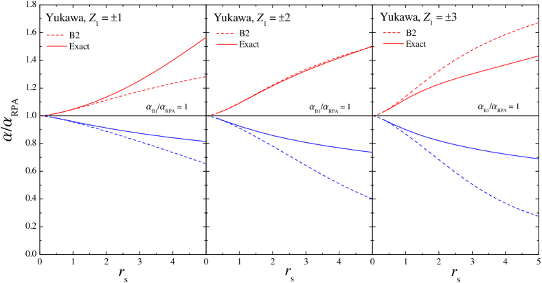
Figure 1: Normalized screening parameter $\alpha/\alpha_{\mathrm{RPA}}$ as a function of $r_{\mathrm{s}}$ for the Yukawa potential and for $Z_{1}=\pm 1,\,\pm 2,\,\pm 3$. Shown are the solutions of Eq. (33) within the B2 approximation (dashed curves) and the exact FSR (17) (solid curves). The horizontal solid line indicates $\alpha_{\mathrm{B}1}/\alpha_{\mathrm{RPA}}=\gamma^{1/2}$ which clearly delimits the domains with positive (upper region) and negative (lower region) values of $Z_{1}$.

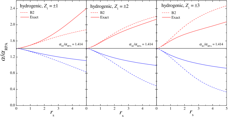
Figure 2: Same as in Fig. 1 but for the hydrogenic potential.

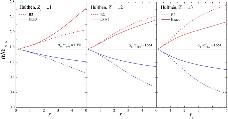
Figure 3: Same as in Fig. 1 but for the Hulthén potential.

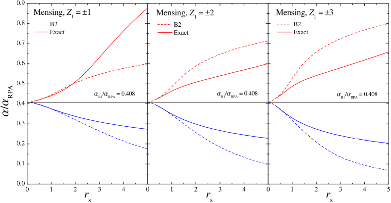
Figure 4: Same as in Fig. 1 but for the Mensing potential.

From Figs. 1–4 it is seen that the B2 screening parameters are in excellent agreement with the exact values when $r_{\mathrm{s}}\lesssim 1$, i.e., at large and moderate electron densities. Moreover, in the extreme regimes with $r_{\mathrm{s}}\to 0$, which are of interest for degenerate astrophysical plasmas, the B1 approximation is increasingly accurate and in this limit both treatments yield $\alpha/\alpha_{\mathrm{RPA}}=\gamma^{1/2}$. In the opposite case of lower densities, $r_{\mathrm{s}}\gtrsim 1$, the B2 approximation deviates from the self-consistent results of the exact FSR but it improves upon the $Z_{1}$-independent $\alpha_{\mathrm{B}1}$. Besides, the B2 approximation underestimates systematically the screening parameter when $Z_{1}<0$ (see Figs. 1–4). In the case of positive ions, however, this approximation generally underestimates $\alpha$ for $Z_{1}=+1$ while overestimating it for $Z_{1}=+2$ and $+3$. Interestingly, the B2 approximation for the Yukawa potential with $Z_{1}=+2$ almost coincides with the exact results (Fig. 1), albeit this is an accidental agreement and is not observed for other potentials. In C we further discuss the B2 approximation for the screening parameter and explore a simple improvement of the model based on the $[1/1]$ Padé approximant.

5 Conclusions

We have proposed a simple way to calculate the static screening parameter (the inverse of the screening length) for an ion in a DEG based on the B2 approximation for the FSR and on the use of this sum rule to adjust in a self-consistent manner the screening parameters of the various interaction potentials. The developed model furnishes a simple scheme to incorporate the effects of the non-linear ion-solid coupling in the quantum formulation of screening and scattering processes, which is regarded an appropriate framework to describe non-linear screening and energy loss of ions in solids.

In the high-density limit ($r_{\mathrm{s}}\lesssim 1$) the present approach agrees excellently with the exact screening parameters calculated self-consistently by imposing the FSR requirement to the numerical phase shifts. At intermediate and small densities ($r_{\mathrm{s}}\gtrsim 1$) our results depart progressively from the exact values but still improve upon the $Z_{1}$-independent predictions of the B1 approximation. More precisely, at $r_{\mathrm{s}}\gtrsim 1$ our model systematically underestimates the screening parameters for negative ions as well as for $Z_{1}=+1$ compared to the exact treatment, while overestimating them for $Z_{1}=+2$ and $+3$.

The Padé approximant to the Born series in the perturbative FSR has been addressed in C as the simplest way to improve the present second-order Born approximation. It is found that the Padé approximant of order $[1/1]$ systematically shifts the perturbative screening parameters towards higher values thus yielding better predictions for any negative ion as well as for $Z_{1}=+1$. Nevertheless, it impairs the agreement with the exact theory for ions with $Z_{1}=+2$ and $+3$.

The model also provides the possibility to calculate the screening parameter of a static impurity ion immersed in a two-dimensional (2D) electron gas. In this case the starting point should be the 2D Schrödinger equation accompanied by an appropriate FSR adapted to the 2D geometry [56]. Moreover, bearing in mind some practical applications the present perturbative formalism can be extended easily to account for the dynamical screening effects of swift ions in solids as proposed in [35]. An expected consequence of the dynamical effects is the replacement of the parameter $\gamma$ and the function $g(u)$ in Eq. (33) by velocity-dependent ones. The validity of the resulting dynamical and perturbative model will be limited by the restriction in the interaction potential, which is usually assumed to maintain the spherical symmetry for a moving ion. However, the self-consistent adjustment of the potential makes this assumption less critical, as may be checked by considering the behavior of the stopping power of the ion in the more unfavorable case of high velocities [35].

Appendix A Evaluation of $g(u)$ for the Mensing potential

In this Appendix we evaluate the function $g(u)$ which determines the second-order correction in the screening parameter (33) for the Mensing potential. Inserting Eq. (52) into Eq. (31) we have

$$g(u)=-\frac{2}{\pi}\int_{0}^{\infty}\ln\left|\frac{z+u}{z-u}\right|\,G^{\prime}(z)\,\mathrm{d}z,$$ (54)

where

$$G(z) = \int_{z}^{\infty}\left[1-j_{0}(x)\right]^{2}\frac{\mathrm{d}x}{x^{3}}$$ (55)

$$= \frac{1}{12z^{2}}\left[2j_{0}(2z)-8j_{0}(z)+3+3j_{0}^{2}(z)\right]$$

$$\mbox{}+\frac{1}{3}\left\{\frac{1}{2}\left[j_{0}^{2}(z/2)-j_{0}^{2}(z)\right]+j_{0}(z)-j_{0}(2z)+\mathop{\mathrm{ci}}\nolimits(2z)-\mathop{\mathrm{ci}}\nolimits(z)\right\}.$$

Here $\mathop{\mathrm{ci}}\nolimits(z)$ is the cosine integral [44, 45]. The explicit form for the function $G(z)$ in Eq. (55) is obtained by standard integration techniques [44, 45]. Next we integrate Eq. (54) by parts and get

$$g(u)=\frac{4u}{\pi}\,\int_{0}^{\infty}\frac{G(z)}{u^{2}-z^{2}}\,\mathrm{d}z.$$ (56)

The singularity at $z=u$ in Eq. (56) must be understood in the sense of Cauchy’s principal value. Further progress is achieved by employing the following integral for $\mathop{\mathrm{ci}}\nolimits(az)$ [45]

$$\frac{2}{\pi}\,\int_{0}^{\infty}\frac{\mathop{\mathrm{ci}}\nolimits(az)}{u^{2}-z^{2}}\,\mathrm{d}z=\frac{1}{u}\,\mathop{\mathrm{si}}\nolimits(au).$$ (57)

Similar integrals can be found in [45] for $j_{0}(az)$ as well as for $j_{0}^{2}(az)$. Then the contribution of the first term (in the square brackets) of Eq. (55) to (56) becomes

$$g_{\mathrm{I}}(u)=\frac{C}{u}+\frac{1}{3\pi u}\,\int_{0}^{\infty}\left[2j_{0}(2z)-8j_{0}(z)+3j_{0}^{2}(z)\right]\frac{\mathrm{d}z}{u^{2}-z^{2}},$$ (58)

where

$$C=\frac{1}{3\pi}\,\int_{0}^{\infty}\left[2j_{0}(2z)-8j_{0}(z)+3+3j_{0}^{2}(z)\right]\frac{\mathrm{d}z}{z^{2}}$$ (59)

is a numerical constant which can be represented in an alternative manner by grouping the different terms in Eq. (59),

$$C=\frac{1}{3\pi}\left\{4\int_{0}^{\infty}\left[1-j_{0}(z)\right]\frac{\mathrm{d}z}{z^{2}}-3\int_{0}^{\infty}\left[1-j_{0}^{2}(z)\right]\frac{\mathrm{d}z}{z^{2}}\right\}.$$ (60)

In Eq. (60) the first and the second integrals are equal to $\pi/4$ and $\pi/3$, respectively [45]. Thus $C=0$ and the function $g_{\mathrm{I}}(u)$ in Eq. (58) is determined by the second term only which, using the known integrals for the spherical Bessel functions [45], is evaluated in the explicit form

$$g_{\mathrm{I}}(u)=\frac{1}{2u^{3}}\,\big{[}1-j_{0}(2u)\big{]}+\frac{1}{3u}\,\big{[}j_{0}^{2}(u)-2j_{0}^{2}(u/2)\big{]}.$$ (61)

The contributions of the other terms of $G(z)$ to $g(u)$ are calculated analogously using Eq. (57) and similar integrals for the spherical Bessel functions. The final result is Eq. (53).

Appendix B Evaluation of $C_{0}$ and $C_{\infty}$ for the Hulthén potential

In the case of the Hulthén potential the evaluation of the constants $C_{0}$ and $C_{\infty}$ is performed using the second equalities of Eqs. (35) and (36) with (50). For $C_{0}$ this yields

$$C_{0}=8\left[h_{3}^{(2)}+3h_{4}^{(1)}-4\zeta(5)\right],$$ (62)

where $h_{r}^{(s)}=\sum_{n=1}^{\infty}n^{-r}H_{n}^{(s)}$ (with positive integers $r\geqslant 2$ and $s$), $H_{n}^{(s)}$ are the so-called harmonic numbers, $H_{n}^{(s)}=\sum_{k=1}^{n}k^{-s}$, and $\zeta(x)$ is the Riemann zeta function. Equation (62) is deduced by making a power series expansion of both functions $\Phi(x)$ and $\Phi(y)$ for the Hulthén potential with respect to $\mathrm{e}^{-x}$ and $\mathrm{e}^{-y}$, respectively [see Eq. (50)]. Inserting these series into Eq. (35) and after a few algebraic manipulations we arrive at Eq. (62). The remaining steps in the derivation of $C_{0}$ are straightforward. First, using an obvious property of the harmonic numbers, $H_{n}^{(s)}=H_{n-1}^{(s)}+n^{-s}$, we see that

$$h_{r}^{(s)}=\zeta(r+s)+\sum_{n=2}^{\infty}\frac{1}{n^{r}}\,H_{n-1}^{(s)}.$$ (63)

Next, applying repeatedly this relation a system of algebraic equations for the three quantities, $h_{2}^{(3)}$, $h_{3}^{(2)}$, and $h_{4}^{(1)}$ can be set up. The solution of this system gives $h_{3}^{(2)}=3\zeta(2)\zeta(3)-(9/2)\zeta(5)$ and $h_{4}^{(1)}=3\zeta(5)-\zeta(2)\zeta(3)$. Inserting these quantities into Eq. (62) we finally arrive at $C_{0}=4\zeta(5)$.

The evaluation of the constant $C_{\infty}$ is facilitated by using the known integral (see, e.g., [45])

$$\Im_{n}(a)=\int_{0}^{\infty}\frac{x^{n}\,\mathrm{d}x}{\mathrm{e}^{ax}-1}=\frac{n!}{a^{n+1}}\,\zeta(n+1),$$ (64)

where $n$ is an arbitrary positive integer and $a>0$. Then $C_{\infty}$ is expressed via $\Im_{1}(a)$ and $\Im_{2}(a)$ as follows

$$C_{\infty}=-2\left[\frac{\mathrm{d}\Im_{1}(a)}{\mathrm{d}a}+\Im_{2}(a)\right]_{a=1}=4\left[\frac{\pi^{2}}{6}-\zeta(3)\right].$$ (65)

Appendix C Padé approximant

The simplest way to improve the B2 approximation is to apply the Padé approximant to the second-order Born series in Eq. (23). Applying the Padé approximant of order $[1/1]$ to this series one finds, instead of Eq. (33),

$$\alpha=\alpha_{\mathrm{RPA}}\,\gamma^{1/2}\left[1-\frac{\pi}{2\gamma}\,Z_{1}\chi^{2}\,g(u)\right]^{-1/2}.$$ (66)

It is now important to trace the basic features of Eq. (66) compared to the standard B2 approximation given by Eq. (33). For a positive ion ($Z_{1}>0$) and at $\chi^{2}\gg 1$ assuming that $\alpha/\alpha_{\mathrm{RPA}}$ increases with $\chi$ (see Figs. 1–4) we get

$$\frac{\alpha}{\alpha_{\mathrm{RPA}}}\simeq\frac{\pi C_{0}}{4\gamma}\,Z_{1}\chi+\sqrt{\gamma+\left(\frac{\pi C_{0}}{4\gamma}\,Z_{1}\chi\right)^{2}}\simeq\frac{\pi C_{0}}{2\gamma}\,Z_{1}\chi.$$ (67)

In the case of a negative ion ($Z_{1}<0$) it is expected that the ratio $\alpha/\alpha_{\mathrm{RPA}}$ decreases with $\chi$ (see Figs. 1–4). Therefore, the solution of Eq. (66) must behave as $\alpha/\alpha_{\mathrm{RPA}}\simeq A(Z_{1})/\chi$ at $\chi^{2}\gg 1$, where $A$ is independent of $\chi$ but depends on $Z_{1}$. The constant $A$ is then extracted from the transcendental equation $A^{2}g(1/A)=\xi\equiv 2\gamma^{2}/\pi|Z_{1}|$. In general the quantity $A$ behaves as $A\sim\xi^{\beta}$, where the numerical constant $\beta$ varies between $1/3\leqslant\beta\leqslant 1$ with increasing $\xi$. The asymptotic solutions of Eq. (66) should be compared with Eqs. (37) and (38). It is seen that the Padé approximant to the Born series in Eq. (23) at $\chi^{2}\gg 1$ increases systematically the screening parameter both for positive and negative ions. Consequently, as discussed above an improvement of the B2 approximation is expected for any negative ion as well as for a positive ion with lowest charge state $Z_{1}=+1$. For $Z_{1}=+2$ and $+3$ it is expected that the Padé approximant to the Born series makes the agreement with the exact treatment even worse. As an example we demonstrate these features in Fig. 5, where the numerical solutions of the approximate Eq. (66) are compared with the exact values for the Yukawa potential. Comparing this figure with Fig. 1 one concludes that the Padé approximant essentially improves the agreement between the B2 approximation and the exact results for any negative ion and in the whole interval of $r_{\mathrm{s}}$. Such an improvement is also clearly visible for $Z_{1}=+1$, while in the case of $Z_{1}=+2$, $+3$ the perturbative approach strongly deviates from the self-consistent treatment based on the FSR.

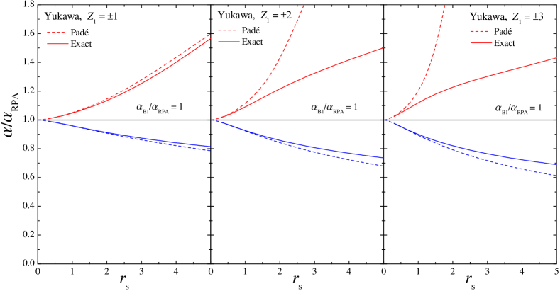
Figure 5: The normalized screening parameter $\alpha/\alpha_{\mathrm{RPA}}$ as a function of the density parameter $r_{\mathrm{s}}$ for the Yukawa potential and for $Z_{1}=\pm 1,\;\pm 2,\;\pm 3$. Shown are the solutions of Eq. (66) (i.e., the Padé approximant of Eq. (23)) (dashed curves) and exact FSR (17) (solid curves). Note that the latter curves as well as the horizontal solid curves are identical to the solid lines shown in Fig. 1.

References

- [1] N.F. Mott, H. Jones, The Theory of the Properties of Metals and Alloys, Dover, New York, 1958.
- [2] M.A. Kumakhov, F.F. Komarov, Energy Loss and Ion Ranges in Solids, Gordon and Breach, New York, 1981.
- [3] J. Lindhard, K. Dan. Vidensk. Selsk. Mat. Fys. Medd. 28 (1954) 1.
- [4] J. Lindhard, A. Winther, K. Dan. Vidensk. Selsk. Mat. Fys. Medd. 34 (1964) 1.
- [5] I. Abril, R. Garcia-Molina, C.D. Denton, F.J. Pérez-Pérez, N.R. Arista, Phys. Rev. A 58 (1998) 357.
- [6] G. Zwicknagel, C. Toepffer, P.G. Reinhard, Phys. Reports 309 (1999) 117.
- [7] H.B. Nersisyan, A.K. Das, Phys. Rev. E 62 (2000) 5636.
- [8] H.B. Nersisyan, A.K. Das, H.H. Matevosyan, Phys. Rev. E 66 (2002) 046415.
- [9] H.B. Nersisyan, A.K. Das, Nucl. Instrum. Methods Phys. Res. B 205 (2003) 281.
- [10] H.B. Nersisyan, A.K. Das, Phys. Rev. E 69 (2004) 046404.
- [11] S. Heredia-Avalos, R. Garcia-Molina, J.M. Fernández-Varea, I. Abril, Phys. Rev. A 72 (2005) 052902.
- [12] H.B. Nersisyan, A.K. Das, in: F. Gerard (Ed.), Interaction of Ion Beams with Plasmas: Energy Loss and Equipartition Sum Rules, Advances in Plasma Physics Research, vol. 6, ch. 2, Nova Science, New York, 2008, p. 81.
- [13] H.B. Nersisyan, A.K. Das, Phys. Rev. E 80 (2009) 016402.
- [14] P.M. Echenique, M.E. Uranga, in: A. Gras-Martí, H.M. Urbassek, N.R. Arista, F. Flores (Eds.), Interaction of Charged Particles with Solids and Surfaces, Plenum Press, New York, 1991.
- [15] P. Sigmund, Phys. Rev. A 26 (1982) 2497.
- [16] L. de Ferrariis, N.R. Arista, Phys. Rev. A 29 (1984) 2145.
- [17] J.S. Briggs, A.P. Pathak, J. Phys. C: Solid State Phys. 7 (1974) 1929; J. Phys. C: Solid State Phys. 6 (1973) L153.
- [18] P.M. Echenique, R.M. Nieminen, R.H. Ritchie, Solid State Commun. 37 (1981) 779.
- [19] P.M. Echenique, R.M. Nieminen, J.C. Ashley, R.H. Ritchie, Phys. Rev. A 33 (1986) 897.
- [20] P.M. Echenique, I. Nagy, A. Arnau, Int. J. Quantum Chem. 23 (1989) 521.
- [21] P.M. Echenique, M.E. Uranga, in: A. Gras-Martí, H.M. Urbassek, N.R. Arista, F. Flores (Eds.), Interaction of Charged Particles with Solids and Surfaces, NATO-ASI Series, vol. B271, Plenum Press, New York, 1991.
- [22] P.F. Meier, Helv. Phys. Acta 48 (1975) 227.
- [23] T.L. Ferrell, R.H. Ritchie, Phys. Rev. B 16 (1977) 115.
- [24] B. Apagyi, I. Nagy, J. Phys. C: Solid State Phys. 20 (1987) 1465.
- [25] A. Ventura, Nuovo Cimento 10D (1988) 43.
- [26] A.H. Sørensen, Nucl. Instrum. Methods Phys. Res. B 48 (1990) 10.
- [27] I. Nagy, Nucl. Instrum. Methods Phys. Res. B 94 (1994) 377.
- [28] B. Apagyi, I. Nagy, J. Phys. C: Solid State Phys. 21 (1988) 3845.
- [29] E.A. Figueroa, N.R. Arista, J. Phys.: Condens. Matter 22 (2010) 015602.
- [30] J. Calera-Rubio, A. Gras-Martí, N.R. Arista, in: R.A. Baragiola (Ed.), Ionization of Solids by Heavy Particles, Plenum Press, New York, 1985, p. 149.
- [31] J. Calera-Rubio, A. Gras-Martí, N.R. Arista, Nucl. Instrum. Methods Phys. Res. B 93 (1994) 137.
- [32] N.-P. Wang, I. Nagy, Phys. Rev. A 56 (1997) 4795.
- [33] E. Zaremba, A. Arnau, P.M. Echenique, Nucl. Instrum. Methods Phys. Res. B 96 (1995) 619.
- [34] I. Nagy, A. Bergara, Nucl. Instrum. Methods Phys. Res. B 115 (1996) 58.
- [35] A.F. Lifschitz, N.R. Arista, Phys. Rev. A 57 (1998) 200.
- [36] I. Nagy, B. Apagyi, Phys. Rev. A 58 (1998) R1653.
- [37] N.R. Arista, A.F. Lifschitz, Nucl. Instrum. Methods Phys. Res. B 193 (2002) 8.
- [38] H.B. Nersisyan, A.K. Das, Nucl. Instrum. Methods Phys. Res. B 227 (2005) 455.
- [39] S.P. Møller, A. Csete, T. Ichioka, H. Knudsen, U.I. Uggerhøj, H.H. Andersen, Phys. Rev. Lett. 88 (2002) 193201.
- [40] S.P. Møller, A. Csete, T. Ichioka, H. Knudsen, U.I. Uggerhøj, H.H. Andersen, Phys. Rev. Lett. 93 (2004) 042502.
- [41] S.P. Møller, A. Csete, T. Ichioka, H. Knudsen, H.-P.E. Kristiansen, U.I. Uggerhøj, H.H. Andersen, P. Sigmund, A. Schinner, Eur. Phys. J. D 46 (2008) 89.
- [42] C.J. Joachain, Quantum Collision Theory, North Holland, Amsterdam, 1975.
- [43] L.D. Landau, E.M. Lifshitz, Quantum Mechanics, Gordon and Breach, New York, 1981.
- [44] M. Abramowitz, I.A. Stegun, Handbook of Mathematical Functions, Dover, New York, 1972.
- [45] I.S. Gradshteyn, I.M. Ryzhik, Table of Integrals, Series and Products, Academic Press, New York, 1980.
- [46] F. Calogero, Variable Phase Approach to Potential Scattering, Academic Press, New York, 1967.
- [47] J. Friedel, Philos. Mag. 43 (1952) 153.
- [48] J. Friedel, Adv. Phys. 3 (1954) 446.
- [49] I. Nagy, B. Apagyi, J.I. Juaristi, P.M. Echenique, Phys. Rev. B 60 (1999) R12546.
- [50] R. Vincent, A. Lodder, I. Nagy, P.M. Echenique, J. Phys.: Condens. Matter 20 (2008) 285218.
- [51] N.R. Arista, P.L. Grande, A.F. Lifschitz, Phys. Rev. A 70 (2004) 042902.
- [52] L. Hulthén, Ark. Mat. Astron. Fys. 28A (1942) 5.
- [53] L. Hulthén, Ark. Mat. Astron. Fys. 29B (1942) 1.
- [54] M.L. Glasser, I. Nagy, J. Math. Chem. 50 (2012) 1707.
- [55] L. Mensing, Z. Phys. 45 (1927) 603.
- [56] F. Stern, W.E. Howard, Phys. Rev. 163 (1967) 816.