Automated polyp detection in colon capsule endoscopy

Abstract

Colorectal polyps are important precursors to colon cancer, a major health problem. Colon capsule endoscopy (CCE) is a safe and minimally invasive examination procedure, in which the images of the intestine are obtained via digital cameras on board of a small capsule ingested by a patient. The video sequence is then analyzed for the presence of polyps. We propose an algorithm that relieves the labor of a human operator analyzing the frames in the video sequence. The algorithm acts as a binary classifier, which labels the frame as either containing polyps or not, based on the geometrical analysis and the texture content of the frame. The geometrical analysis is based on a segmentation of an image with the help of a mid-pass filter. The features extracted by the segmentation procedure are classified according to an assumption that the polyps are characterized as protrusions that are mostly round in shape. Thus, we use a best fit ball radius as a decision parameter of a binary classifier. We present a statistical study of the performance of our approach on a data set containing over $18,900$ frames from the endoscopic video sequences of five adult patients. The algorithm demonstrates a solid performance, achieving $47\%$ sensitivity per frame and over $81\%$ sensitivity per polyp at a specificity level of $90\%$. On average, with a video sequence length of $3747$ frames, only $367$ false positive frames need to be inspected by a human operator.

I Introduction

Colorectal cancer is the second most common cause of cancer in women and the third most common cause in men [18], with the mortality reaching to about $50\%$ of the incidence. Colorectal polyps are important precursors to colon cancer, which may develop if the polyps are left untreated. Colon capsule endoscopy (CCE) [1, 8, 9, 12, 17, 24, 25, 26, 29] is a feasible alternative to conventional examination methods, such as the colonoscopy or computed tomography (CT) colonography [10].

In CCE a small imaging device, a capsule, is ingested by the patient. As the capsule passes through the patient’s gastrointestinal tract, it records the digital images of the surroundings by means of an on-board camera (or multiple cameras). As the images are recorded, they are transmitted wirelessly to a recording device carried by the patient. Depending on the model of the capsule and its regime of operation, the images are captured at a rate ranging from 2 to 30 or more frames per second, with the low frame rate devices being prevalent currently. After the whole video sequence is recorded, it has to be analyzed for the presence of polyps. The video sequence of examination of a single patient may contain thousands of frames, which makes manual analysis of all frames a burdensome task. Using an automated procedure for detecting the presence of polyps in the frames can greatly reduce such burden. Thus, an efficient algorithm should not only be able to detect the polyps accurately (high sensitivity), but should also have a reasonably low rate of false positive detections (high specificity) to minimize the number of frames that have to be analyzed manually.

In this paper we provide an efficient algorithm for detecting polyps in CCE video frame sequences. The performance of the algorithm is assessed on a relatively diverse data set, which ensures that no over-fitting takes place. The paper is organized as follows. The main idea and its comparison to existing approaches is discussed in section II. The steps of the algorithm are described in detail in section III, which concludes with a summary of the algorithm. We test our algorithm on a data set comprised of the frames from the endoscopic video sequences of five adult patients. In section IV the data set and testing methodology are presented. It is followed by the results of the testing in section V. Finally, we conclude with the discussion of the results and some directions for future research in section VI.

II Binary classifier with pre-selection

The proposed algorithm of polyp detection is based on extracting certain geometric information from the frames captured by the capsule endoscope’s camera. Such approach is not new, as it has been noticed before that the polyps can be characterized as protrusions from the surrounding mucosal tissue [11, 20, 30, 31, 32], which was used in CT colonography and in the analysis of conventional colonoscopy videos [4, 5, 22, 23, 27]. Thus, it is natural to compute some measure of protrusion and try to detect the frames containing polyps as the ones for which such measure is high. However, this leads to an issue that was also observed in the above mentioned works. The issue is distinguishing between the protrusions that are polyps and the numerous folds of healthy mucosal tissue. This problem can be alleviated by some form of image segmentation that takes place prior to the computation of the measure of protrusion [6], which is what we do in this work as well.

A particular choice of a measure of protrusion is of crucial importance. Many authors have proposed the use of principal curvatures and the related quantities, such as the shape index and curvedness [33], or the Gaussian and mean curvatures [11]. The main disadvantage of such approaches is that the computation of the curvatures is based on differentiation of the image, which must be approximated by finite differences. In the presence of noise these computations are rather unstable, which requires some form of smoothing to be applied to the image first. However, even if the image is smoothed before computing the finite differences, the curvatures are still sensitive to small highly curved protrusions that are unlikely to correspond to polyps. Thus, in this work we use a more globalized measure of protrusion, the radius of the best fit ball. A similar sphere fitting approach was used in the CT colonography setting in [19]. In our approach we do not do the fitting to the image itself, but we first apply a certain type of a mid-pass filter to it. This allows us to isolate the protrusions withing certain size limits. We use the radius of the best fit ball as the decision parameter in a binary classifier. If the decision parameter is larger than the discrimination threshold, then the frame is classified as containing a polyp.

Another feature that distinguishes our approach from the ones mentioned above is the use of texture information. The surface of polyps is often highly textured, so it makes sense to discard the frames with too little texture content in them. On the other hand, too much texture implies the presence of bubbles and/or trash liquids in the frame. These unwanted features may lead a geometry-based classifier to classify the frame as containing a polyp when no polyp is present, i.e. they lead to an increased number of false positives. Thus, in order to avoid both of the situations mentioned above, we apply a pre-selection procedure that discards the frames with too much or too little texture content. Combined with the binary classifier this gives the algorithm that we refer to as binary classification with pre-selection.

III Details of the algorithm

In the section below we present the detailed step-by-step description of the algorithm of processing of single frames from a capsule endoscope video sequence. The algorithm makes a decision for every frame whether to classify it either as containing polyps (“polyp” frame) or as containing normal tissue only (“normal” frame).

Besides the frame to be processed, the algorithm accepts as the inputs a number of numerical parameters that have to be chosen in advance. The choice of these parameters and the robustness of the algorithm with respect to the changes in them is addressed in section IV-C. For the purpose of numerical experiments, the values of these parameters were chosen manually. Ideally, we would like to have a systematic way to calibrate our algorithm, i.e. to assign the optimal values to the parameters based on the algorithm’s performance for some calibration data set. Currently, we do not have such a procedure, so this remains one of the topics of future research discussed in section VI.

Another choice that requires a separate study is the choice of the color space of the frame. In this work we convert the captured color frames to grayscale before processing. This choice provides good polyp detection results, as we observe from the numerical experiments in section V. However, we believe that certain improvements in this area are possible. For example, the polyps are often highly vascularized, so one would expect them to have a stronger red color component. Thus, one may use a measure of red color content in the frame, like the $a$ component of the $Lab$ color space [16], in polyp detection. Here we rely mostly on the geometrical information for polyp detection, but our algorithm could still be supplemented by the use of color information.

III-A Pre-processing

Since the capsule endoscope operates in an absence of ambient light, an on-board light source is used to capture the images. Because of the directional nature of the light source and the optical properties of the camera’s lens, the captured frames are often subject to an artifact known as vignetting, which refers to the fall-off of intensity of the captured frame away from its center. As a first step of frame pre-processing we perform the normalization of intensity using the vignetting correction algorithm of Y. Zheng et al. [34]. Performance of the intensity normalization procedure is illustrated in Figure 1 (c).

The images acquired by the endoscope are of circular shape. The area of the rectangular frame outside the circular mask is typically filled with a solid color. This creates a discontinuity along the edge of the circular mask, which may cause problems in the subsequent steps of the algorithm. To remove this discontinuity we use a simple linear extrapolation to extend the values from the interior of a circular mask to the rest of the rectangular frame.

This is accomplised by solving the linear system which corresponds to an upwind discretization of the following PDE

$$\nabla{\bf f}\cdot\vec{{\bf r}}=1,$$ (1)

assuming that the frame ${\bf f}$ is given on a $N_{y}\times N_{x}$ uniform Cartesian grid. Here the vector field $\vec{{\bf r}}$ at the pixel $(i,j)$ is the unit vector

$$\vec{{\bf r}}_{ij}=\frac{1}{\sqrt{(i-N_{y}/2)^{2}+(j-N_{x}/2)^{2}}}\begin{bmatrix}i-N_{y}/2\\ j-N_{x}/2\end{bmatrix}.$$ (2)

With the values of ${\bf f}$ inside the circular mask fixed, the solution outside the mask provides the desired extrapolated values. To obtain the resulting linear system we use a standard upwind discretization scheme; see e.g. [13].

The linear extrapolation is shown in Figure 1 (d), where the radius of a circular mask $R_{mask}$ is taken to be slightly less than half the frame size. All the subsequent calculations involving the extrapolated frame are subject to masking after the calculation is done. This removes the effects that the artifacts of extrapolation (seen as light radial strips in the right corners of Figure 1 (d)) might have on the result.

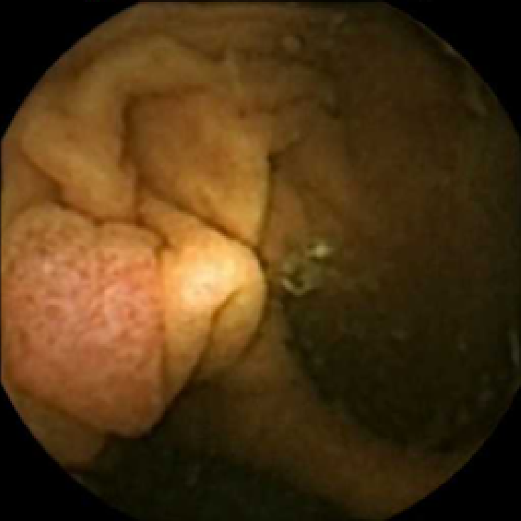
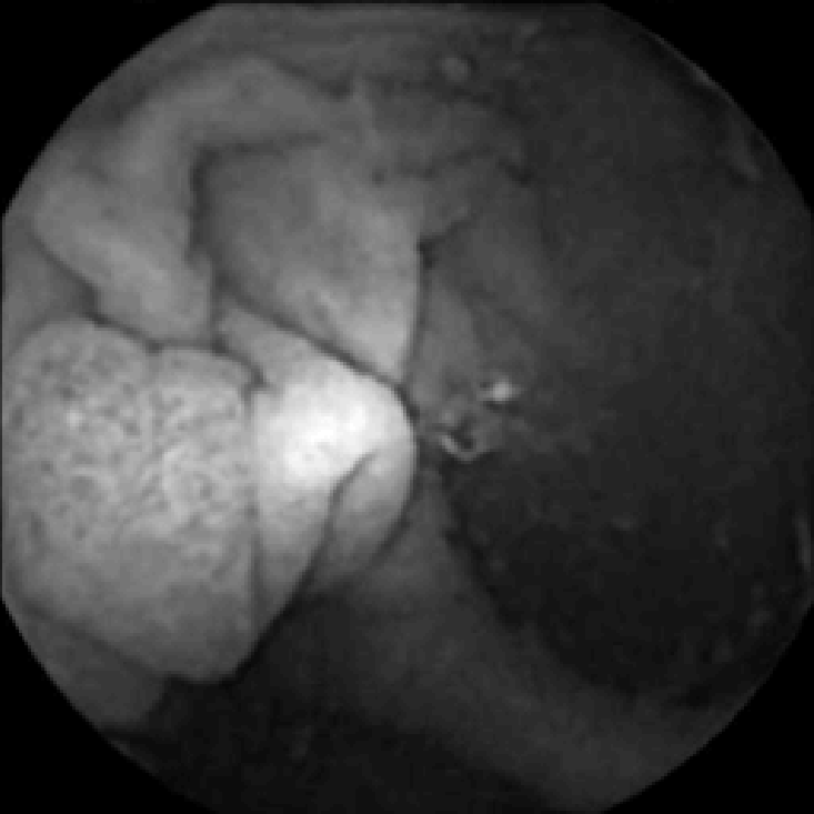
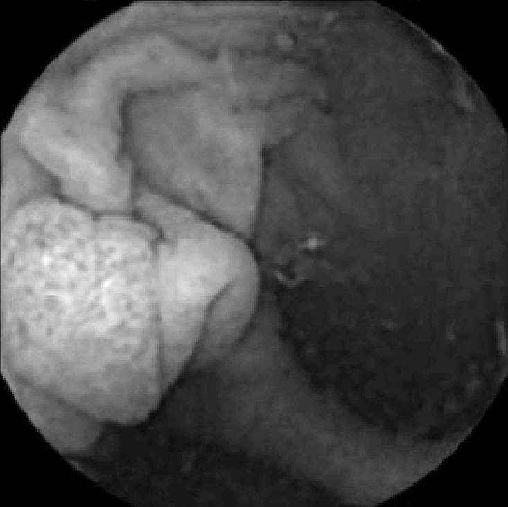
(a)	(b)	(c)
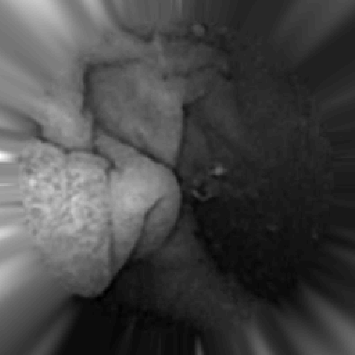
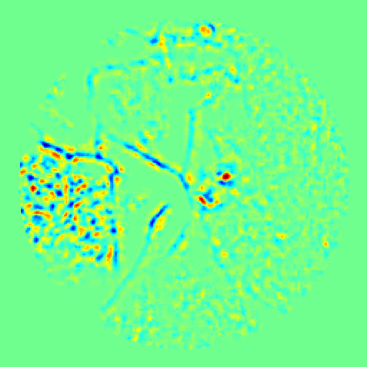
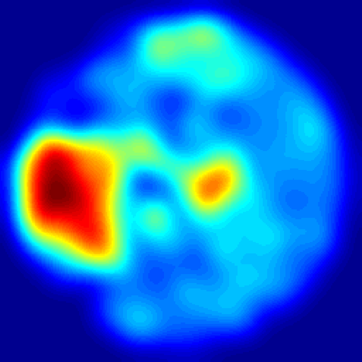
(d)	(e)	(f)
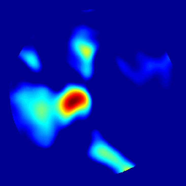
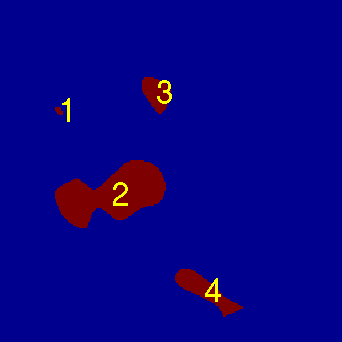
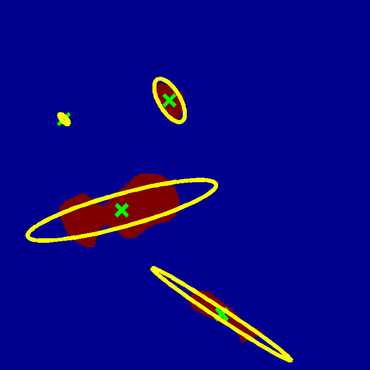
(g)	(h)	(i)

Figure 1: Steps of the algorithm for a polyp frame: (a) original color frame, (b) frame in grayscale, (c) normalized intensity, (d) pre-processed frame ${\bf f}$: extension by linear extrapolation, (e) texture ${\bf t}$, (f) non-linear convolution-type transform ${\bf T}$ of the texture, (g) mid-pass filtering ${\bf u}$, (h) segmentation ${\bf s}$ with $N_{C}=4$ connected components ${\bf s}^{(k)}$ numbered $k=1,\ldots,N_{C}$, (i) ellipses of inertia $r^{(k)}(\theta)$ (yellow) with the centers of mass $(c_{x}^{(k)},c_{y}^{(k)})$ given by green $\times$.

III-B Texture computation and convolution

Computation of the texture content in the frame is an important first step of the algorithm. We use the thresholding on the texture content as a pre-selection criterion, i.e. some frames are discarded from the consideration (and labeled as “normal”) based on the texture content alone.

To separate the pre-processed frame ${\bf f}$ into the texture ${\bf t}$ and cartoon ${\bf c}$ components

$${\bf f}={\bf t}+{\bf c},$$ (3)

we use an algorithm of Buades et al. [3]. The algorithm is based on iterative application of low-pass filtering by convolution with a Gaussian kernel. As its input parameters it accepts the number of iterations $n_{iter}$ and the standard deviation $\sigma_{t}$ of the Gaussian kernel in pixels. Hereafter, we treat the frame as a matrix ${\bf f}\in\mathbb{R}^{N_{y}\times N_{x}}$, where $N_{x}$ is the width and $N_{y}$ is the height of the frame in pixels. The individual pixels are denoted by $f_{ij}$, $1\leq i\leq N_{y}$, $1\leq j\leq N_{x}$. The quantities having the same dimensions as the frame itself (${\bf t}$, ${\bf c}$, etc.) are treated the same way and are denoted by bold symbols. Their individual pixels are denoted by regular symbols with indices $i$ and $j$, i.e. $t_{ij}$, $c_{ij}$, etc.

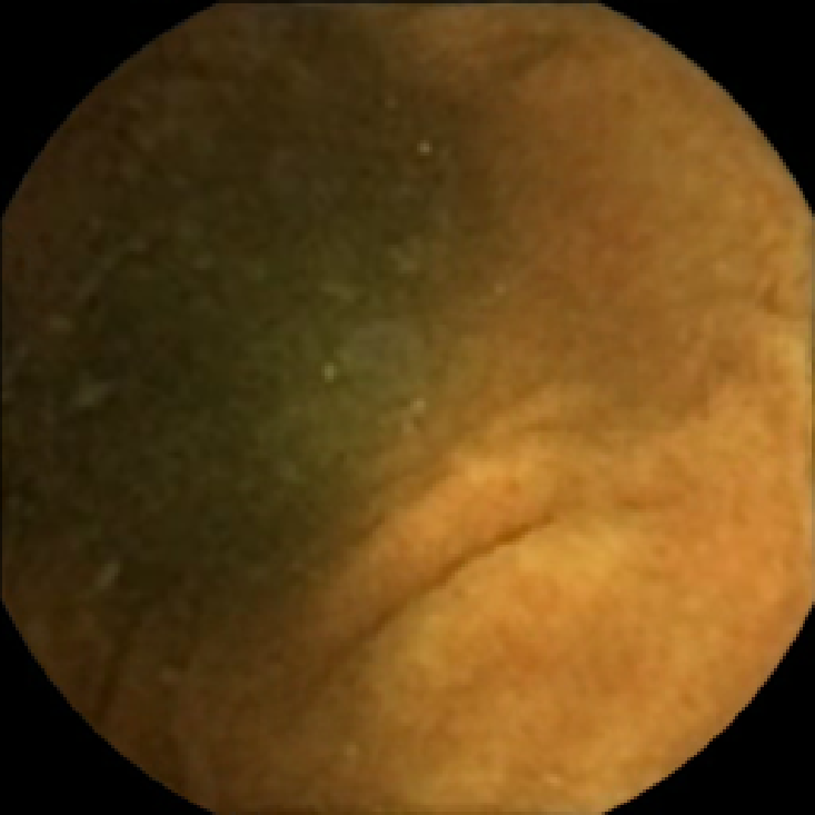
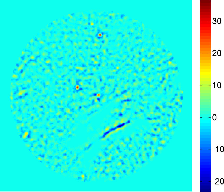
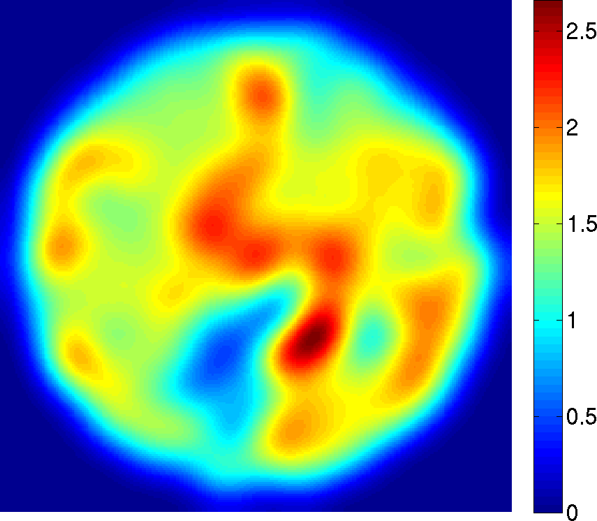
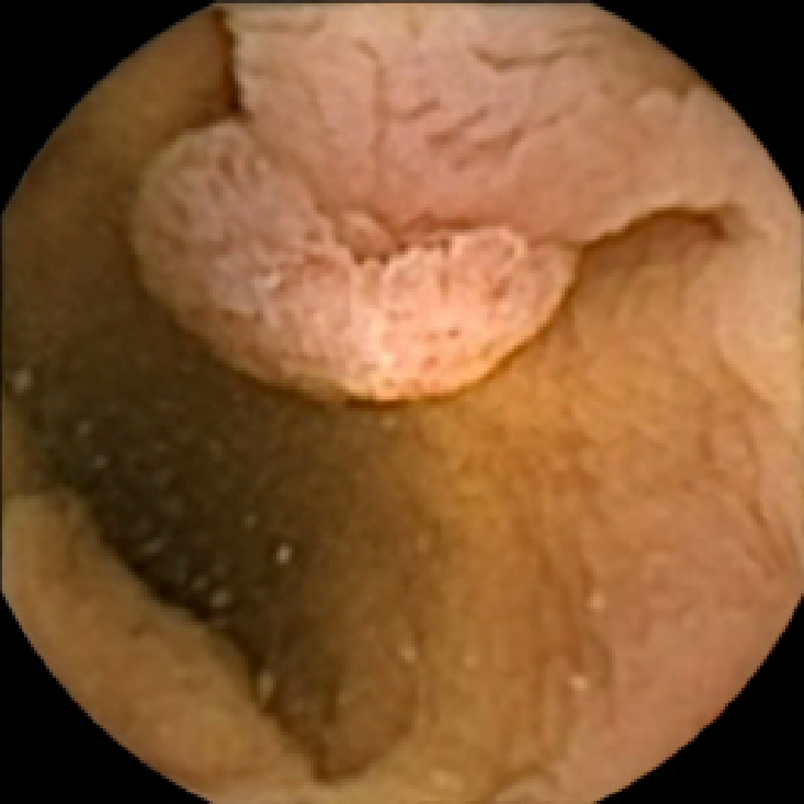
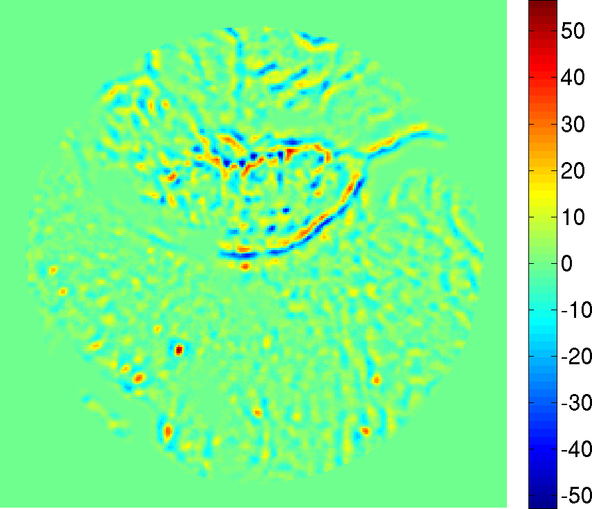
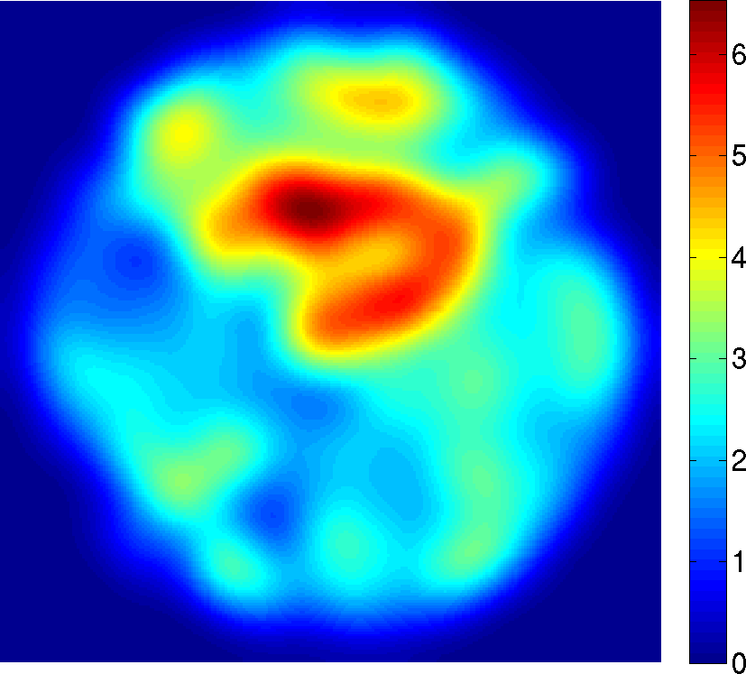
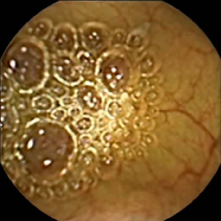
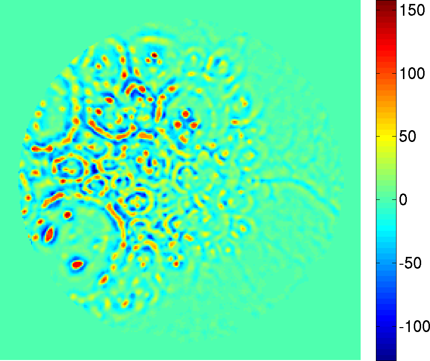
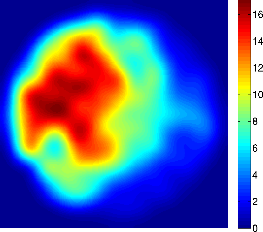
(a)	(b)	(c)

Figure 2: Texture computation for the cases of low (top row, $T_{max}=2.6$), medium (middle row, $T_{max}=6.5$) and high (bottom row, $T_{max}=17.1$) texture content. Top and bottom rows are normal frames, middle row is a polyp frame. Columns: (a) original frames, (b) texture ${\bf t}$, (c) convolution-type transform ${\bf T}$.

The use of texture in pre-selection is motivated by two considerations. First, the surface of polyps is often textured, so discarding the frames with low texture content helps to distinguish the polyp frames from the frames with flat mucosa. Second, when trash liquids or bubbles are present in the frame, most of ${\bf f}$ ends up in ${\bf t}$, so we expect the texture content to be abnormally high in this case. Since detecting polyps in the frames polluted with trash or bubbles is not feasible anyway, we may as well discard the frames with very high texture content. Another reason to discard such frames is that the mid-pass filtering (see section III-C) that we use in polyp detection is sensitive to the presence of large areas covered with trash and bubbles. If such frames are not discarded, this may result in an increased number of false positives.

Once we have a decomposition (3), we need to define a measure of texture content that would be appropriate for performing the pre-selection. The measure should be more sensitive to the presence of large textured regions and less sensitive to small regions even if those are strongly textured, since those typically correspond to occasional trash liquids or bubbles. Thus, we perform the following non-linear convolution-type transform of the texture

$${\bf T}=L_{\sigma}(|{\bf t}|^{p}),$$ (4)

where the absolute value and exponentiation in $|{\bf t}|^{p}$ are pixel-wise, and $L_{\sigma}$ is a linear operator convolving the frame with a Gaussian kernel with standard deviation $\sigma$. The operator $L_{\sigma}$ is also used in mid-pass filtering in the next step of the algorithm, and is defined as follows. First, we define a one-dimensional Gaussian kernel on a stencil of $2\lceil\sigma\rceil+1$ pixels, normalized so that it sums to one. Then we perform a convolution of the rows of the frame with the one-dimensional kernel. Finally, the columns of the row-convolved frame are convolved with the same kernel. When the stencil of the one-dimensional kernel protrudes outside the frame, we use mirror boundary conditions.

The usage of convolution in (4) with $\sigma$ equal to a half of a typical polyp size in pixels, allows to emphasize the textured regions that are likely to be polyps. Adding non-linearity in the form of exponentiation with $p<1$ de-emphasizes small regions with strong texture. This is illustrated in Figure 1 (e) and (f), where ${\bf t}$ and ${\bf T}$ are shown respectively. We observe that there are two well-pronounced bumps in ${\bf T}$. A larger in size and magnitude on the left corresponds to the polyp, a smaller one in the middle-right is due to a few bubbles present in the frame.

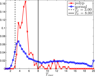
Figure 3: Histogram of the distribution of $T_{max}$ for normal and polyp frames.

Once the non-linear transform (4) is calculated, we can compute the measure of texture content

$$T_{max}=\mathop{\mbox{max }}\limits_{i,j}T_{ij},\quad 1\leq i\leq N_{y},\;1\leq j\leq N_{x}.$$ (5)

Then the pre-selection criterion is a simple thresholding

$$T_{L}\leq T_{max}\leq T_{U}.$$ (6)

The lower bound filters out the frames with too little texture content that are unlikely to contain any polyps due to most polyps having a textured surface. The upper bound allows us to discard the frames polluted with trash and bubbles, since even if they contain polyps, they are likely to be obscured. This is illustrated in Figure 2, where we display two normal frames with low and high values of $T_{max}$ and a polyp frame with a medium value of $T_{max}$. As expected, the first normal frame containing flat mucosa has little texture content. The second normal frame polluted with bubbles has strong texture content in the bubbles area, which is especially pronounced in the plot of ${\bf T}$. Finally, the polyp frame has moderately textured polyp area, which can also be easily observed from ${\bf T}$ that has the strongest feature in that region.

To verify the above conclusions statistically, we compare in Figure 3 the histograms of the distributions of $T_{max}$ for normal and polyp frames in our test data set (see section IV-A for a detailed description). We observe that the peak of the histogram for normal frames is shifted towards the lower values of $T_{max}$, which explains the effectiveness of the lower threshold. For high values of $T_{max}$ the histogram for normal frames is consistently well above the one for the polyp frames, indicating a large number of frames polluted with trash and bubbles. Given such distributions of $T_{max}$, the pre-selection criterion (6) appears quite effective. For the values of parameters given in Table I, exactly $90\%$ of the polyp frames pass the pre-selection, while only $47.84\%$ of the normal frames do so.

III-C Mid-pass filtering and segmentation

After the frame passes the pre-selection, we identify certain regions that may correspond to polyps. An essential feature of polyps is that they are protrusions or bumps on a flatter surrounding tissue. The purpose of this step is to detect such geometric features. Note that the polyps have a certain range of characteristic dimensions. Thus, in order to detect possible polyps, the geometrical processing should act as a mid-pass filter that filters out the features that are too small or too large. Here we use a mid-pass filter of the form

$${\bf u}=H({\bf w})\cdot{\bf w},$$ (7)

where ${\bf w}$ is defined by

$${\bf w}=\frac{L_{\sigma_{1}}({\bf f})}{L_{\sigma_{2}}({\bf f})}-1,$$ (8)

and $H$ is the Heaviside step function

$$H(x)=\left\{\begin{tabular}[]{ll}0,&if $x<0$,\\ 1,&if $x\geq 0$.\end{tabular}\right.$$ (9)

The application of $H$, multiplication and division in (7) are pixel-wise. The standard deviations of the convolution operators satisfy $\sigma_{1}<\sigma_{2}$. They correspond to the typical radii (in pixels) of the polyps that we expect to detect. Note that measuring the polyp size in pixels is sensitive to the distance between the polyp and the camera, especially when such distance is large. This may lead to failure to detect the polyps which size in pixels is small. Here we rely on the fact that the polyp is likely to be present in a number of consecutive frames as the capsule moves along. Thus, the polyp will be observed from different distances including some that are small enough to make the pixel size sufficient for producing a detectable feature in the mid-pass filtered frame ${\bf u}$.

We use a ratio in (7) instead of a difference to obtain a quantity that depends less on the absolute prominence of the protrusion, but more on its relative prominence compared to the surrounding tissue. This allows for a better detection of flat polyps. Also, the difference of Gaussians is known to be subject to the scaling effect [21] similarly to the Laplacian of a Gaussian. However, the ratio in (8) is invariant under the scaling of the image ${\bf f}$, thus the scaling effect does not apply in our case.

Since the convolution with a smaller standard deviation is in the numerator of (8), the protrusions correspond to large positive values of ${\bf w}$, hence we only use of the positive part of ${\bf w}$ in (7).

In Figure 1 (g) we show the result of mid-pass filtering ${\bf u}$. We observe several features present in ${\bf u}$ with the most prominent one corresponding to a polyp. To perform the binary classification we need to assign a numerical quantity to each of these features that would determine how likely does each of them correspond to a polyp.

To separate the features from each other we use a binary segmentation via thresholding

$${\bf s}=H({\bf u}-\Theta)\in\{0,1\}^{N_{y}\times N_{x}},$$ (10)

where $H$ is taken pixel-wise and the scalar threshold $\Theta$ is defined by

$$\begin{split}\Theta=&\mbox{max}\left(\mbox{min}\left(\frac{1}{2}\mathop{\mbox{max}}\limits_{i,j}u_{ij},M_{U}\right),M_{L}\right),\\ &1\leq i\leq N_{y},\;1\leq j\leq N_{x},\end{split}$$ (11)

with some bounds $M_{U}>M_{L}>0$. This means that the threshold $\Theta$ is taken to be a half of maximum value of ${\bf u}$, unless it goes above $M_{U}$ or below $M_{L}$, in which case it defaults to the corresponding bound.

An example of a binary segmentation ${\bf s}$ obtained with (10) is shown in Figure 1 (h), where four features can be seen. By features we mean the connected components of ${\bf s}$, which can be found using an algorithm by Haralick and Shapiro [14]. It provides a decomposition

$${\bf s}=\sum_{k=1}^{N_{C}}{\bf s}^{(k)},$$ (12)

where $N_{C}$ is the total number of connected components in ${\bf s}$, and ${\bf s}^{(k)}$ are the disjoint connected components. The pixel values $s_{ij}^{(k)}$ of ${\bf s}^{(k)}$ are defined as

$$s_{ij}^{(k)}=\left\{\begin{tabular}[]{ll}1,&\begin{tabular}[]{l}if pixel $(i,j)$ belongs to the\\ $k^{th}$ connected component,\end{tabular}\\ 0,&\begin{tabular}[]{l}otherwise.\end{tabular}\end{tabular}\right.$$ (13)

Decomposition (12) is illustrated in Figure 1 (h), where the four features ${\bf s}^{(k)}$ are numbered $k=1,\ldots,N_{C}$ in the order they are found by the algorithm.

III-D Geometrical processing and the tensor of intertia

After the binary segmentation of the frame is decomposed into separate features (12), we can process them individually to determine which of them might correspond to polyps. The simplest criterion we can apply is filtering the features by their sizes

$$K_{S}=\left\{k\in\{1,2,\ldots,N_{C}\}\;|\;S_{L}\leq S^{(k)}\leq S_{U}\right\},$$ (14)

where the size $S^{(k)}$ of the $k^{th}$ feature is defined by

$$S^{(k)}=\sum_{i,j}s_{ij}^{(k)},\quad k=1,\ldots,N_{C}.$$ (15)

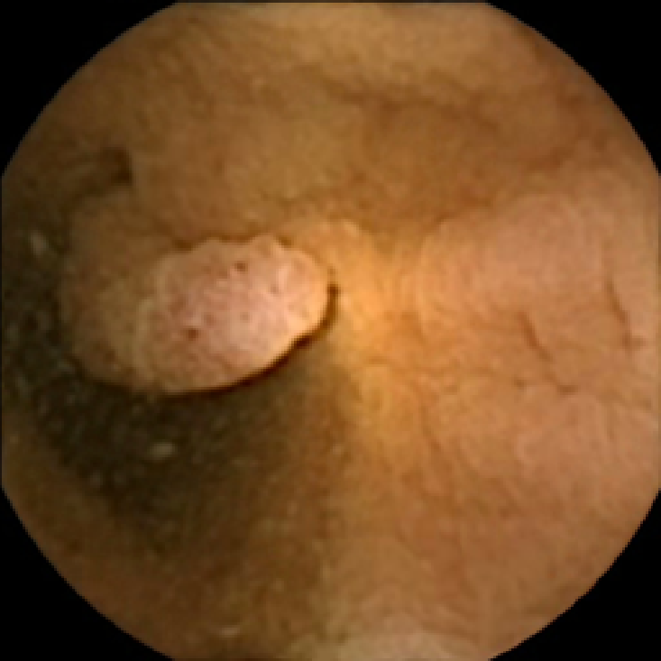
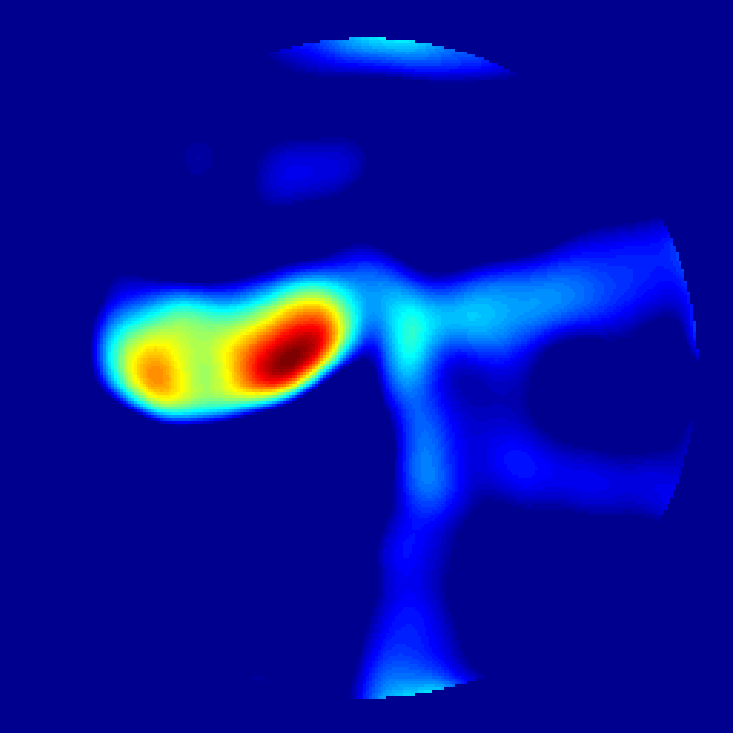
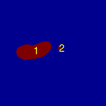
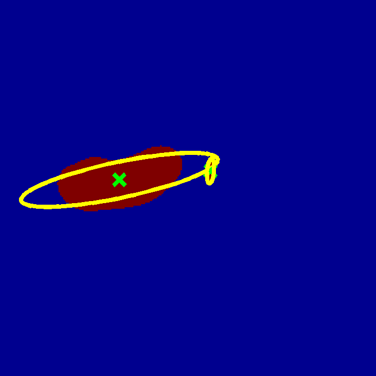
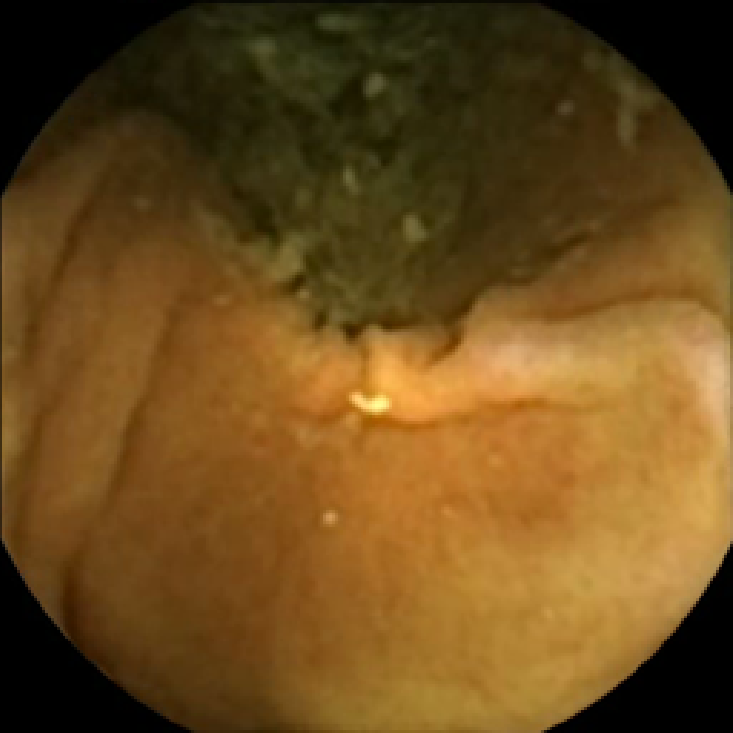
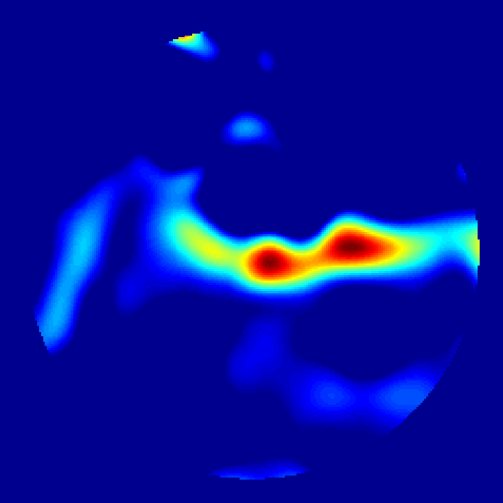
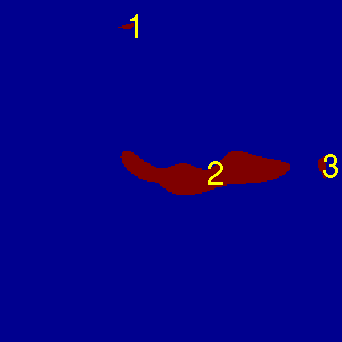
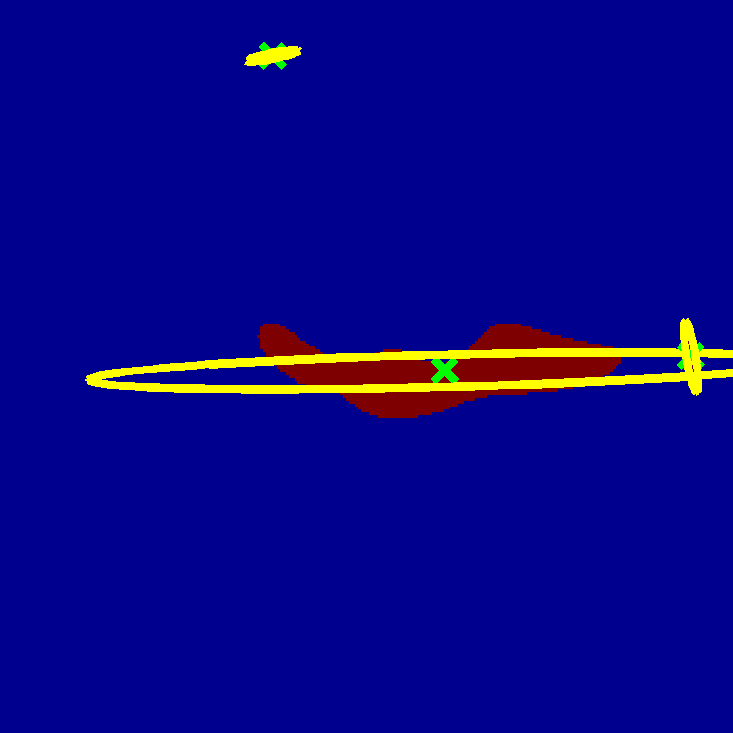
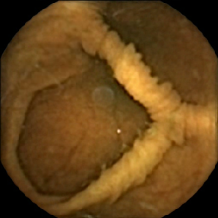
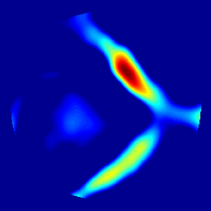
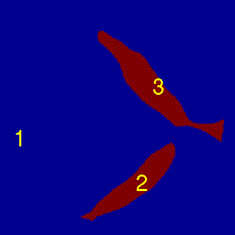
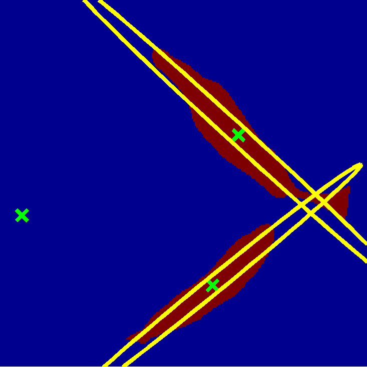
(a)	(b)	(c)	(d)

Figure 4: Comparison of the geometrical processing and the tensor of inertia calculation for a polyp frame (first row) and two normal frames (second and third rows). Columns: (a) original frames, (b) mid-pass filtering ${\bf u}$, (c) binary segmentation ${\bf s}=\sum_{k=1}^{N_{C}}s^{(k)}$, (d) ellipses of inertia $r^{(k)}(\theta)$ (yellow) with the centers of mass $(c_{x}^{(k)},c_{y}^{(k)})$ given by green $\times$.

Features that are too large, typically correspond to folds of normal mucosal tissue. Very small features are likely to be the artifacts of mid-pass filtering and the subsequent segmentation. The above feature size criterion can be used to discard such features.

A more sophisticated criterion that can help to eliminate the non-polyp features that pass the size criterion (14) is based on the computation of the features’ tensors of inertia [28] to determine how stretched the feature is. For this we define the matrices

$$\begin{split}x^{(k)}_{ij}=&\left\{\begin{tabular}[]{ll}$j$,&if $s^{(k)}_{ij}=1$\\ $0$,&if $s^{(k)}_{ij}=0$\end{tabular}\right.,\\ y^{(k)}_{ij}=&\left\{\begin{tabular}[]{ll}$i$,&if $s^{(k)}_{ij}=1$\\ $0$,&if $s^{(k)}_{ij}=0$\end{tabular}\right.,\\ &1\leq i\leq N_{y},\;1\leq j\leq N_{x},\end{split}$$ (16)

that allow us to compute first the centers of mass

$$\begin{split}c_{x}^{(k)}=&\frac{1}{S^{(k)}}\sum\limits_{i,j}x^{(k)}_{ij},\\ c_{y}^{(k)}=&\frac{1}{S^{(k)}}\sum\limits_{i,j}y^{(k)}_{ij},\\ &k=1,\ldots,N_{C}.\end{split}$$ (17)

Then we can define the tensors of inertia $I^{(k)}\in\mathbb{R}^{2\times 2}$ as

$$\begin{split}I^{(k)}=&\sum_{i,j}\begin{bmatrix}\left(\widehat{y}^{(k)}_{ij}\right)^{2}&-\widehat{x}^{(k)}_{ij}\widehat{y}^{(k)}_{ij}\\ -\widehat{x}^{(k)}_{ij}\widehat{y}^{(k)}_{ij}&\left(\widehat{x}^{(k)}_{ij}\right)^{2}\end{bmatrix},\\ &k=1,\ldots,N_{C},\end{split}$$ (18)

where $\widehat{x}^{(k)}_{ij}=x^{(k)}_{ij}-c_{x}^{(k)}$ and $\widehat{y}^{(k)}_{ij}=y^{(k)}_{ij}-c_{y}^{(k)}$ are the coordinates relative to the centers of mass. The tensors of inertia are symmetric positive definite, thus they can be used to define ellipses. Using an analogy from the classical mechanics, we refer to these ellipses as the ellipses of inertia. The eccentricities $E^{(k)}$ of such ellipses are given by

$$E^{(k)}=\frac{\lambda^{(k)}_{max}}{\lambda^{(k)}_{min}},\quad k=1,\ldots,N_{C},$$ (19)

where $\lambda^{(k)}_{max}\geq\lambda^{(k)}_{min}>0$ are the eigenvalues of $I^{(k)}$. The eccentricity $E^{(k)}$ determines how much is the $k^{th}$ feature stretched in one direction compared to its transversal. This information is useful for our purposes, since we expect the polyps to be more round in shape than the mucosal folds, that are often stretched.

We illustrate the above considerations in Figure 4, where we compare the ellipses of inertia for a polyp frame and two frames with pronounced mucosal folds. The ellipses we plot are

$$r^{(k)}(\theta)=\sqrt{\frac{S^{(k)}}{\pi\lambda_{max}^{(k)}\lambda_{min}^{(k)}}}\;I^{(k)}\begin{pmatrix}\cos\theta\\ \sin\theta\end{pmatrix}+\begin{pmatrix}c^{(k)}_{x}\\ c^{(k)}_{y}\end{pmatrix},$$ (20)

where $\theta\in[0,2\pi]$. The scaling term in front of $I^{(k)}$ is chosen so that the area of the ellipse of inertia is the same as the size $S^{(k)}$ of the corresponding feature.

As expected, we observe that the ellipses corresponding to mucosal folds (feature 2 in the second row and features 2 and 3 in the third row of Figure 4) are indeed much more stretched out than the ellipse corresponding to a polyp (feature 1 in the first row of Figure 4). Stretched ellipses imply higher eccentricity, thus we impose the following criterion

$$K_{E}=\left\{k\in\{1,2,\ldots,N_{C}\}\;|\;E^{(k)}\leq E_{max}\right\}$$ (21)

with some threshold $E_{max}$ to select moderately stretched features that are more likely to correspond to polyps.

The combined geometric criterion is

$$K_{G}=K_{S}\cap K_{E}.$$ (22)

If none of the features in the frame passes this criterion, i.e. if $K_{G}=\varnothing$, then the frame is labeled as normal. If one or more features satisfy (22), then we continue to the next step, where we compute a parameter upon which we base the decision whether the frame is classified as containing polyps or not.

III-E Decision parameter and binary classifier

The final step of the algorithm is the computation of the decision parameter that we use in the binary classification. This parameter is geometrical in nature and we define it as follows.

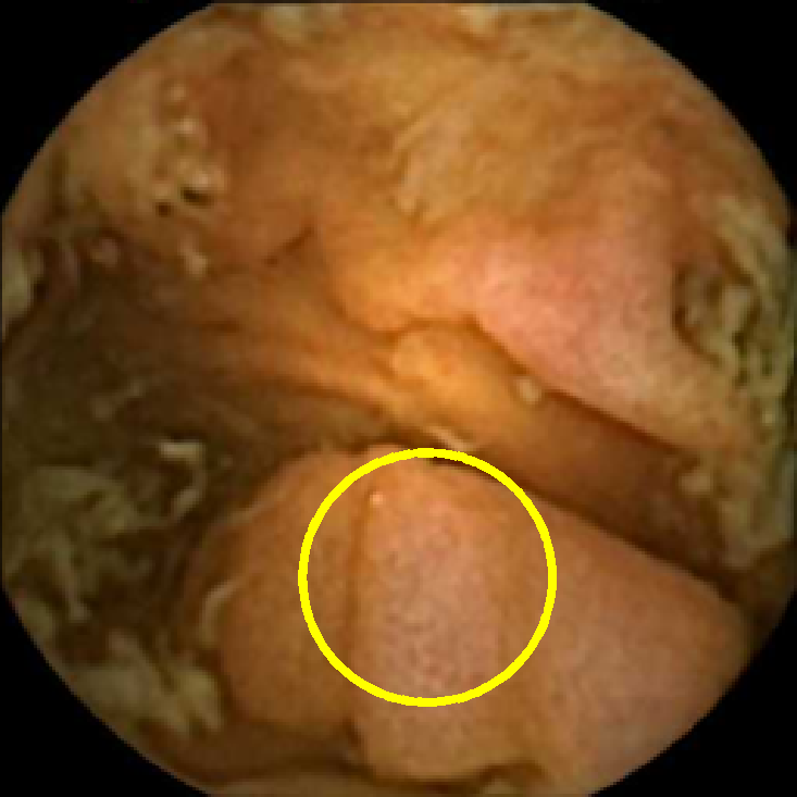
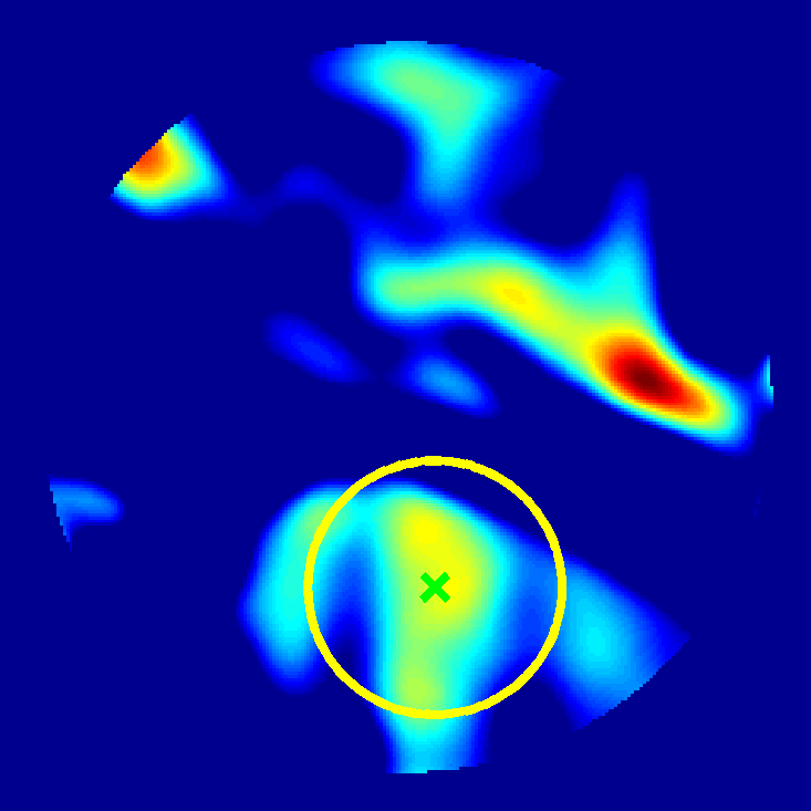
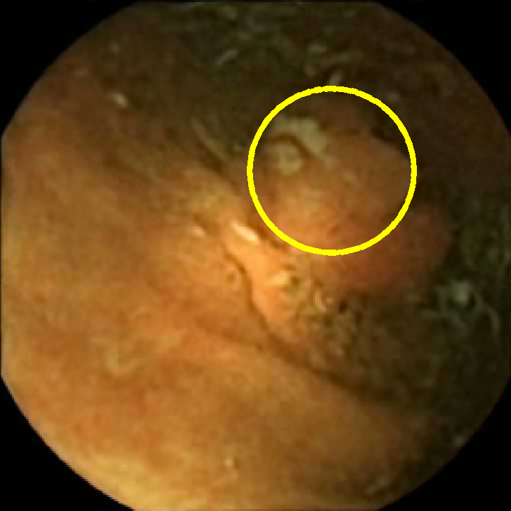
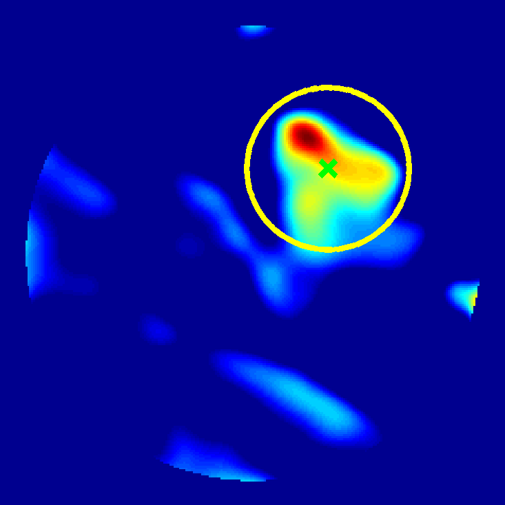
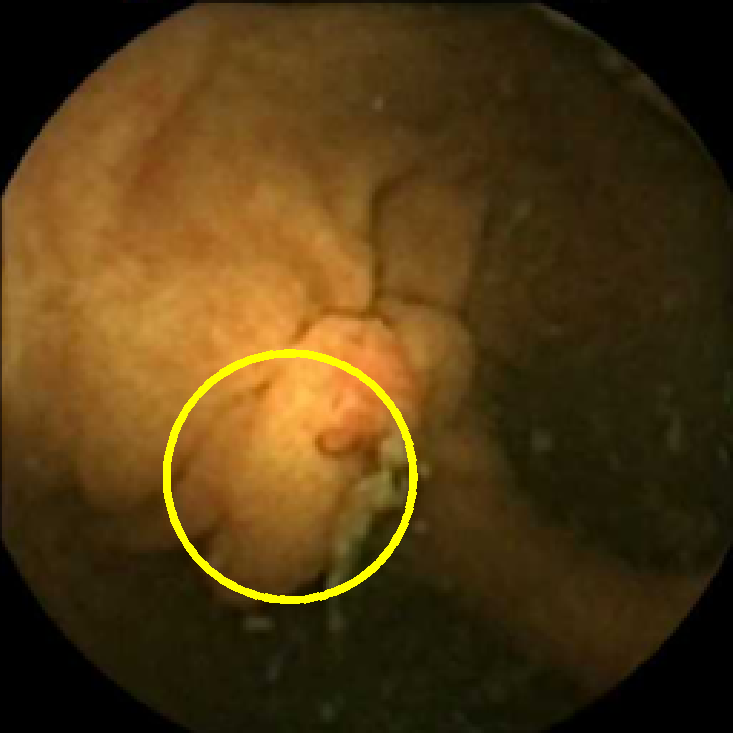
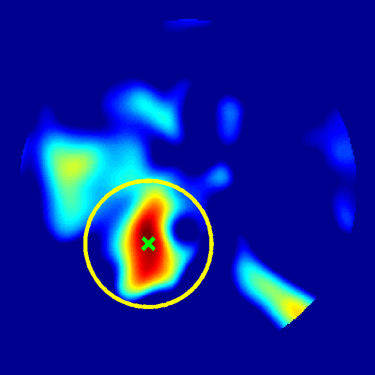
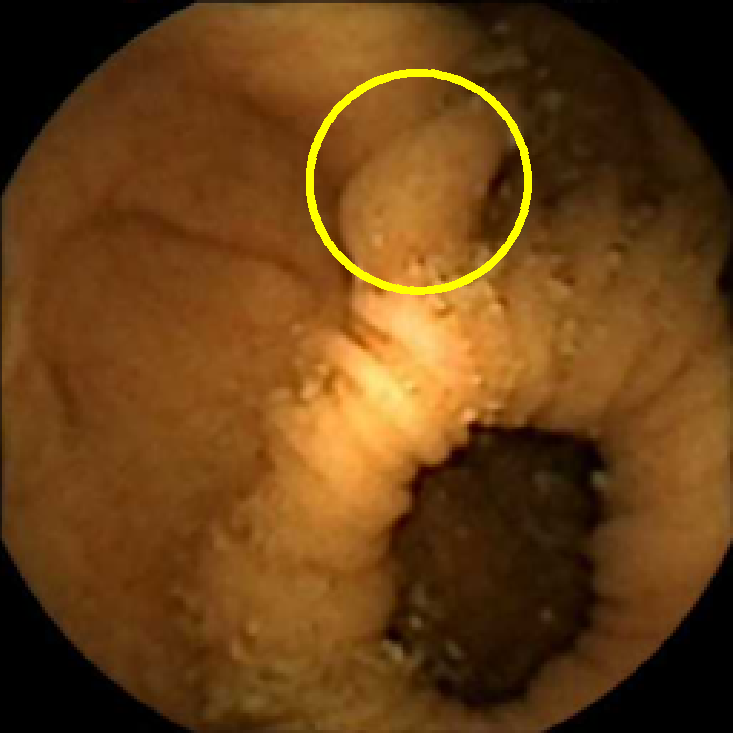
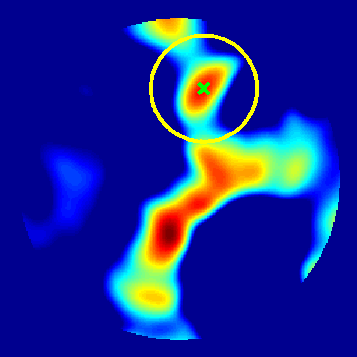
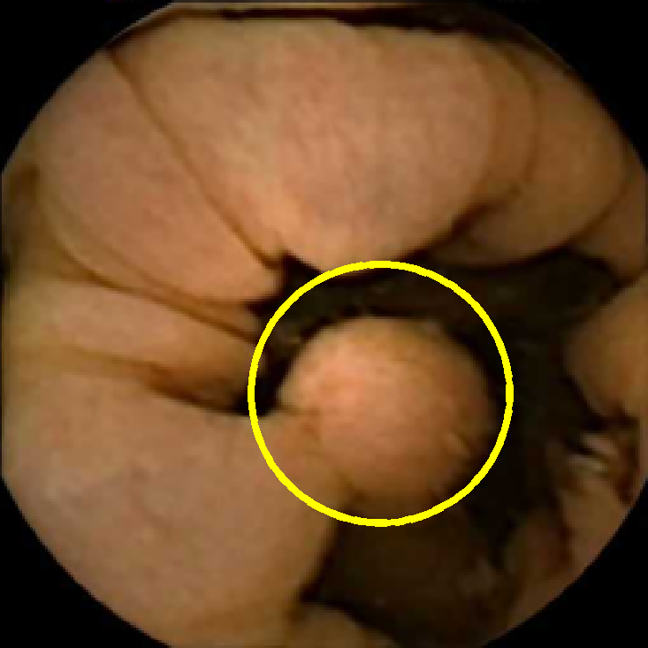
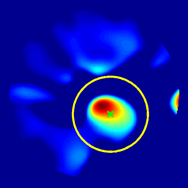
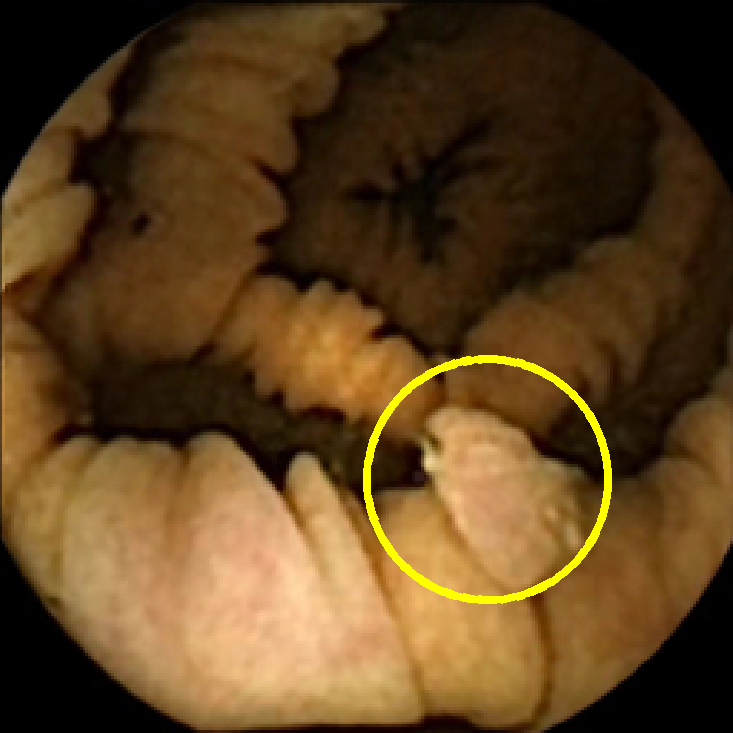
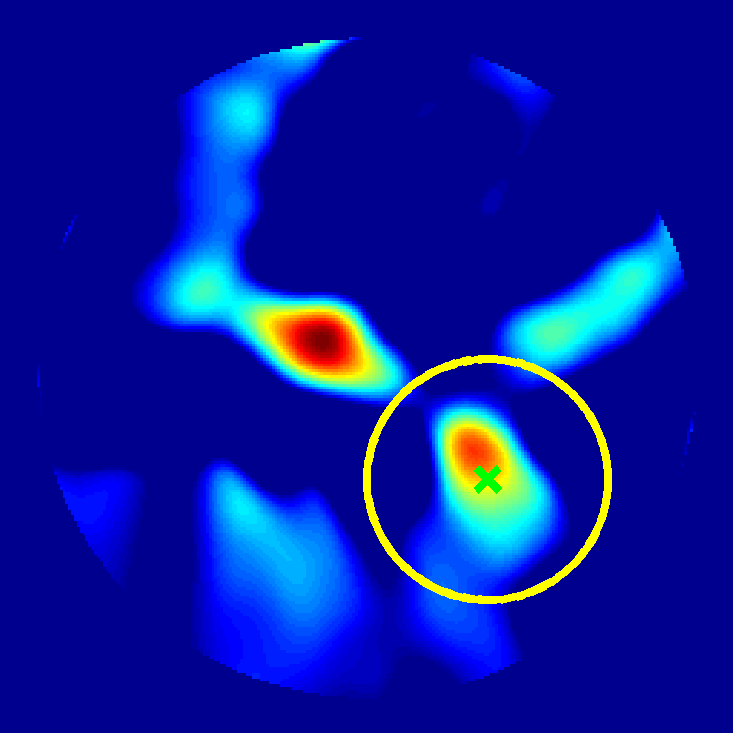
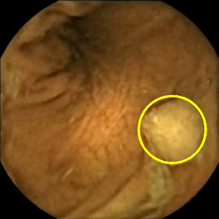
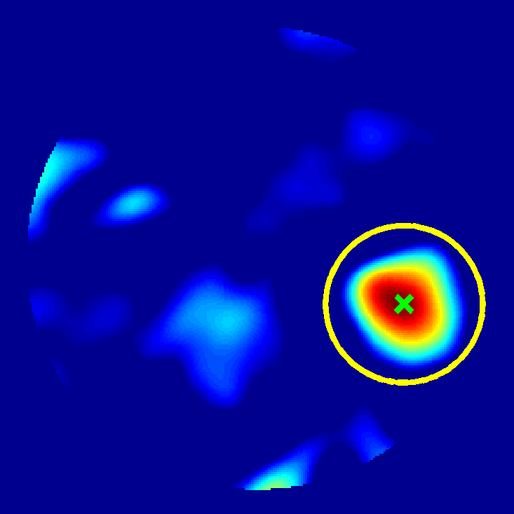
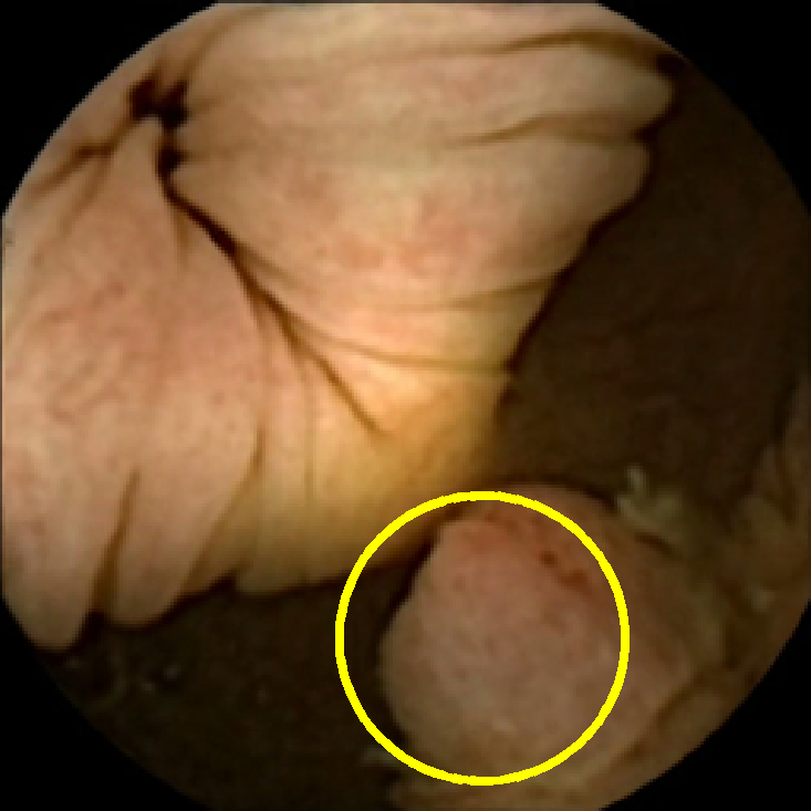
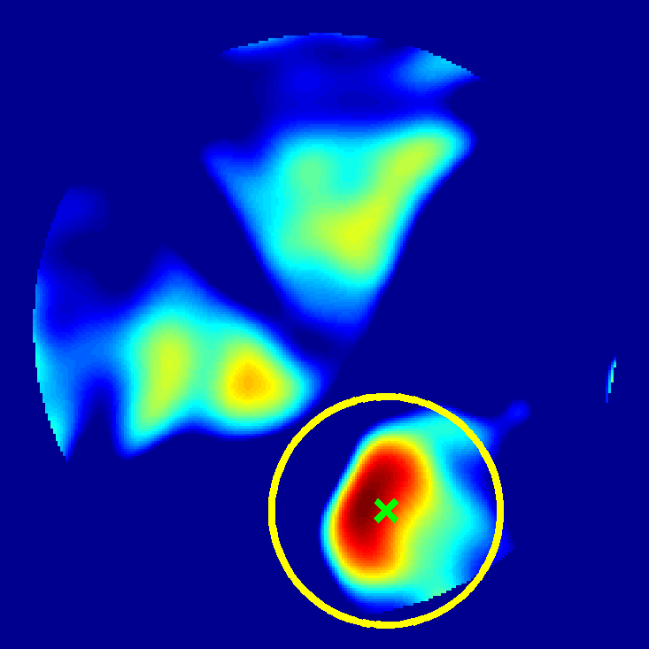
(a)	(b)	(c)	(d)

Figure 5: Optimal fit balls for some of the correctly classified polyps. The circles of optimal radii $R_{max}$ (yellow) are superimposed on original polyp frames (columns (a) and (c)) and on the corresponding mid-pass filtered images ${\bf u}$ (columns (b) and (d)). In columns (b) and (d) the centers of mass ($\widetilde{c}_{x}^{(k)}$, $\widetilde{c}_{y}^{(k)}$) are marked by green $\times$.

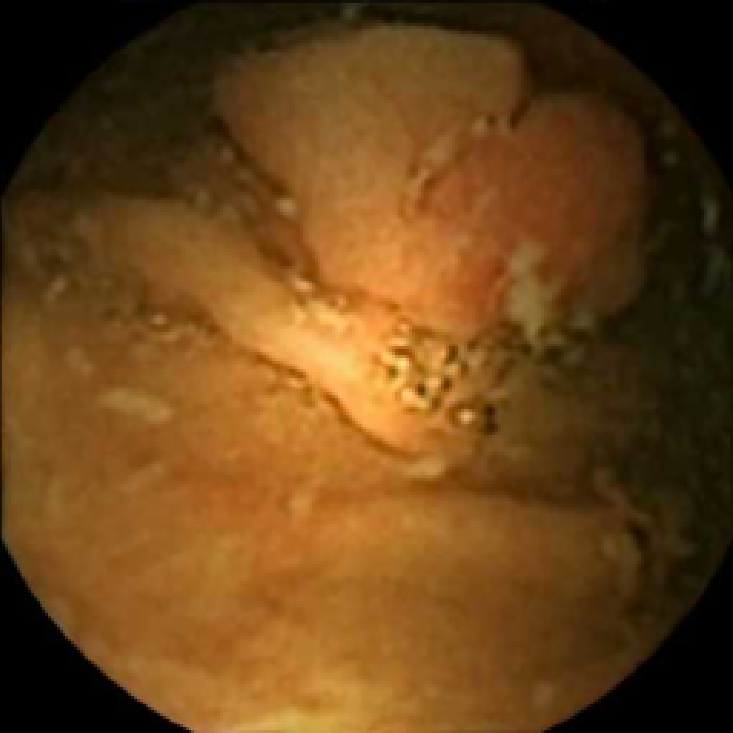
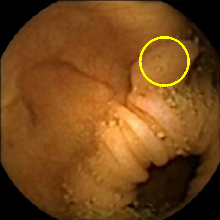
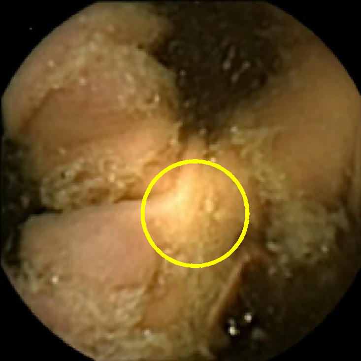
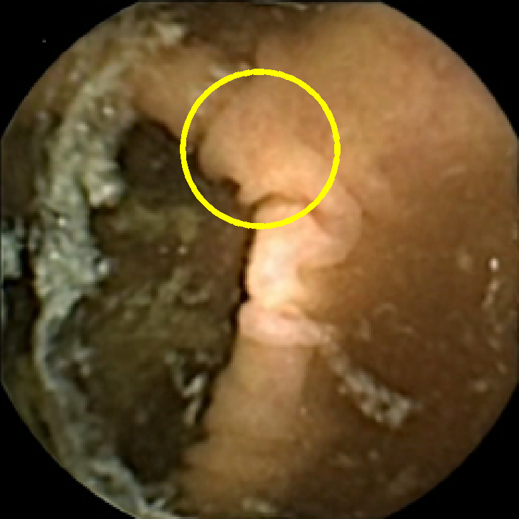
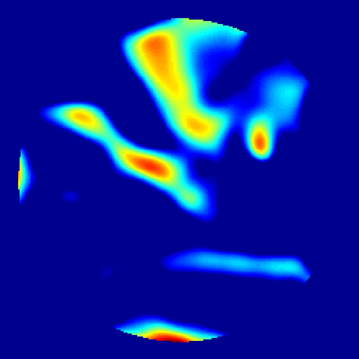
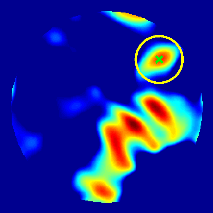
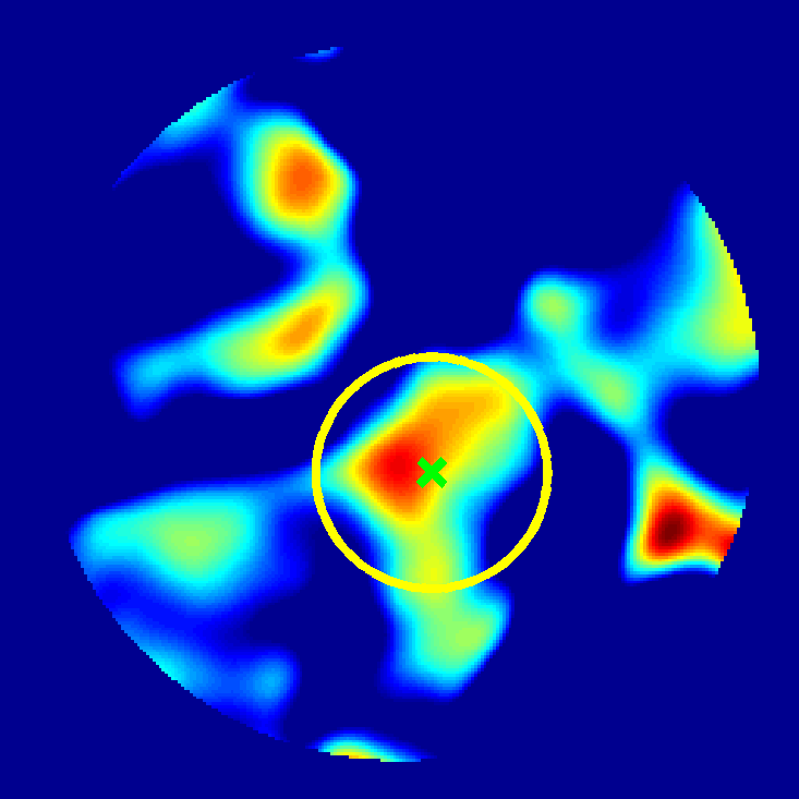
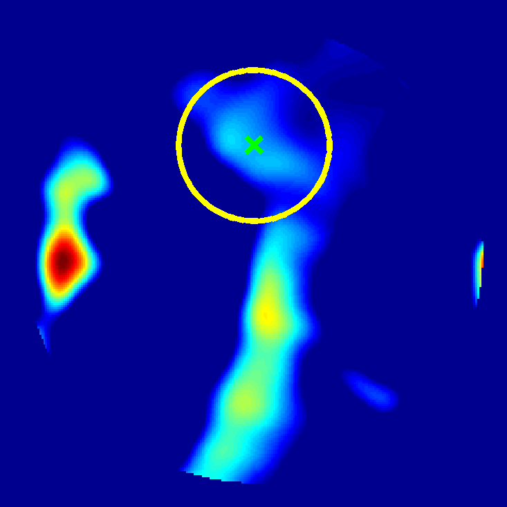
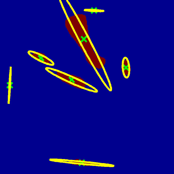
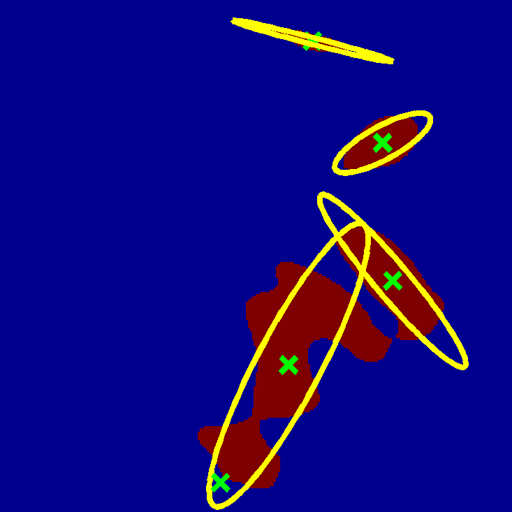
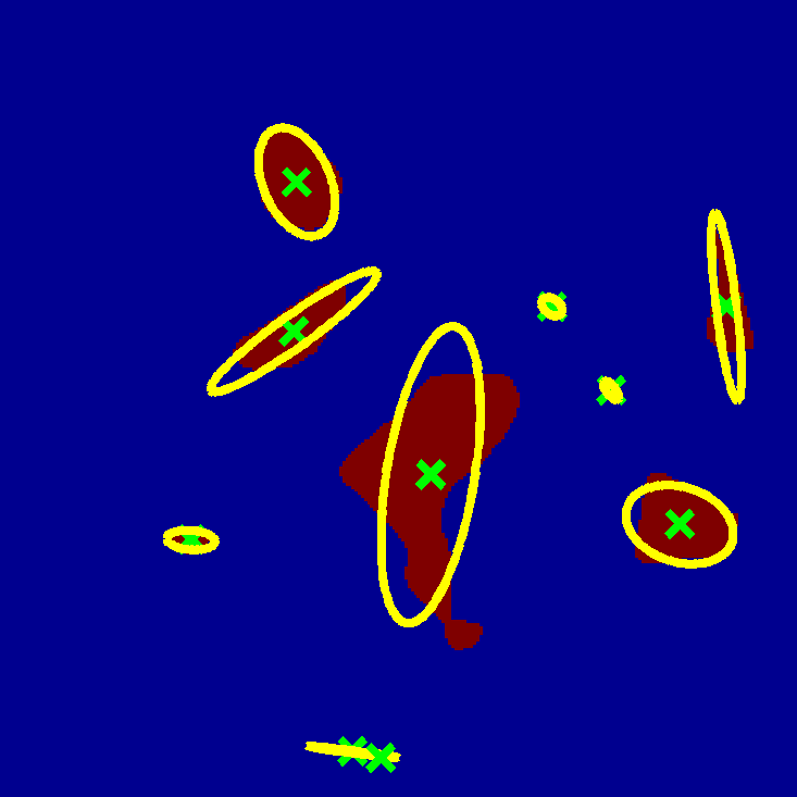
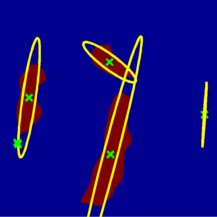
(a)	(b)	(c)	(d)

Figure 6: Incorrectly classified frames. False negatives: columns (a) and (b). False positives: columns (c) and (d). Top row: original frames with superimposed circles of radii $R_{max}$. Middle row: mid-pass filtered images ${\bf u}$ with superimposed circles of radii $R_{max}$. Bottom row: binary segmentation ${\bf s}=\sum_{k=1}^{N_{C}}s^{(k)}$ with superimposed ellipses of inertia $r^{(k)}(\theta)$.

First, we compute the centers of mass using ${\bf u}$ masked with ${\bf s}^{(k)}$ instead of just (17), which gives

$$\widetilde{c}_{x}^{(k)}=\frac{1}{U^{(k)}}\sum_{i,j}x_{ij}^{(k)}u_{ij},\quad\widetilde{c}_{y}^{(k)}=\frac{1}{U^{(k)}}\sum_{i,j}y_{ij}^{(k)}u_{ij},$$ (23)

for $k\in K_{G}$, where

$$U^{(k)}=\sum_{i,j}u_{ij}s_{ij}^{(k)},\quad k\in K_{G},$$ (24)

and the matrices $x^{(k)}$, $y^{(k)}$ are defined in (16).

Second, we place a ball with a center at $(\widetilde{c}_{x}^{(k)},\widetilde{c}_{y}^{(k)})$ and we search of the radius of such ball so that it fits best the mid-pass filtered image ${\bf u}$. The radius of this ball will be the decision parameter in our binary classification. Such definition of the decision parameter is motivated by the same considerations as the criterion (22), i.e. we expect the polyps to be the protrusions that are somewhat rounded. Note that the combined geometric criterion (22) only uses the two-dimensional information in ${\bf u}$ by only working with the binary segmentation ${\bf s}$. To utilize information about the height of the protrusions, we need to work with ${\bf u}$ itself, which is why we fit the ball to ${\bf u}$ instead of ${\bf s}$.

To compute the optimal fit ball radius we define the matrix-valued functions

$$\begin{split}b_{ij}^{(k)}(R)=&\frac{1}{N_{x}^{2}}\left(R^{2}-(i-\widetilde{c}_{y}^{(k)})^{2}-(j-\widetilde{c}_{x}^{(k)})^{2}\right),\\ &1\leq i\leq N_{y},\;1\leq j\leq N_{x},\end{split}$$ (25)

and their positive parts

$$\widetilde{{\bf b}}^{(k)}(R)=H({\bf b}^{(k)}(R))\cdot{\bf b}^{(k)}(R),\quad k\in K_{G},$$ (26)

where Heaviside step function and the multiplication are performed pixel-wise.

Then for each feature we can define the radius of the ball that provides the best fit of ${\bf u}$ as a solution of a one-dimensional optimization problem

$$R_{opt}^{(k)}=\mathop{\mbox{argmin }}\limits_{R}\|{\bf u}-\widetilde{{\bf b}}^{(k)}(R)\|_{F},\quad k\in K_{G},$$ (27)

where $\|.\|_{F}$ is the matrix Frobenius norm. Since the objective in the optimization problem (27) is cheap to evaluate, the problem can be easily solved by a simple one-dimensional search over the integer values in some interval, which we take here to be $\left[1,\lfloor N_{x}/3\rfloor\right]$.

Finally, we can define the decision parameter by taking the maximum of the optimal fit ball radii over all the features that pass the combined geometric criterion (22) as

$$R_{max}=\mathop{\mbox{max }}\limits_{k\in K_{G}}R_{opt}^{(k)}.$$ (28)

For the frames with $K_{G}=\varnothing$ we set $R_{max}=0$. To account for the pre-selection criterion (6), we also set $R_{max}=0$ for the frames with $T_{max}<T_{L}$ or $T_{max}>T_{U}$.

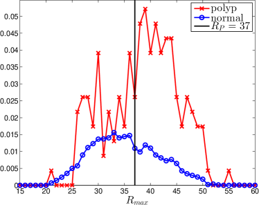
Figure 7: Histogram of the distribution of $R_{max}$ for normal and polyp frames after passing the pre-selection (6) and satisfying the combined geometric criterion (22).

Since we expect the polyps to correspond to more pronounced round protrusions, we define the binary classifier as

$$BC({\bf f})=\left\{\begin{tabular}[]{ll}``polyp'',&if $R_{max}\geq R_{P}$\\ ``normal'',&if $R_{max}<R_{P}$\end{tabular}\right..$$ (29)

Obviously, the performace of the classifier depends dramatically on the choice of the discrimination threshold value $R_{P}$. This choice is discussed in detail in section IV-B, where we use statistical analysis to determine the value of $R_{P}$ that provides the desired performance.

In Figure 5 we show the circles of radius $R_{max}$ corresponding to the features that were correctly classified as polyps by (29). We observe that the classifier was able to identify the polyps of a variety of shapes even in the presence of small amounts of trash liquid (first row) or when the polyps are located next to mucosal folds (rows two to four in column (c)).

The examples of incorrect classification of frames are presented in Figure 6. The first two examples show false negatives, each highlighting a possible source of classification error. The example in column (a) shows the case where the feature corresponding to the polyp was too stretched out and thus was rejected by the eccentricity criterion (21). In contrast, the feature corresponding to the polyp in column (b) has passed the combined geometric criterion (22), but the radius $R_{max}$ was below the threshold $R_{P}=37$ of the binary classifier. Examples in columns (c) and (d) show the two sources of possible false positives. The false positive detection in column (c) is due to insufficient illumination correction. The bright spot is not fully corrected at the pre-processing stage and subsequently generates a polyp-like feature in the mid-pass filtered frame that happens to pass through all the criteria. Finally, in column (d) a mucosal fold is classified as polyp. Note that such cases are the most difficult to deal with, as the mucosal folds can often be hard to distinguish from polyps even for a human operator.

The overall good performance of the classifier can be explained by statistical considerations. In Figure 7 we show the histogram of the distribution of $R_{max}$ for normal and polyp frames in our test data set (see section IV-A for the detailed description). We observe that the peak of the distribution of $R_{max}$ for polyp frames is shifted to the right compared to the peak of the distribution for “normal”, non-polyp frames. Note that overall the distribution for normal frames is well below the distribution for the polyp frames. This is due to setting $R_{max}$ to zero for the frames that do not pass the pre-selection or that do not satisfy the combined geometric criterion.

III-F Summary of the algorithm

Figure 8: The flow of the data in Algorithm 1.

After establishing the main steps of the algorithm, we are ready to summarize the processing of a single frame in a video sequence. The processing algorithm accepts the frame as an input and gives the classification “polyp” or “normal” as an output. The flow of data in the algorithm is illustrated in Figure 8.

Algorithm 1 (Binary classification with pre-selection).

1. Pre-processing. Convert the frame to grayscale, perform the intensity normalization, apply the linear extension outside the circular mask of radius $R_{mask}$ to obtain the pre-processed frame ${\bf f}$.

2. Texture analysis. Compute the texture ${\bf t}$ from (3) and its non-linear convolution-type transform ${\bf T}$ using (4). Find the maximum $T_{max}$ of ${\bf T}$ and apply the pre-selection criterion (6). If the frame fails the criterion, set $R_{max}=0$ and go to step 6, otherwise continue.

3. Mid-pass filtering and segmentation. Apply the mid-pass filter (7) to obtain ${\bf u}$ and perform the binary segmentation (10) of ${\bf u}$ to obtain ${\bf s}$. Decompose the binary image ${\bf s}$ into connected components ${\bf s}^{(k)}$, $k=1,\ldots,N_{C}$ that correspond to $N_{C}$ “features” present in the frame.

4. Geometric analysis. For each of $N_{C}$ features compute the tensor of inertia $I^{(k)}$ via (18) and the eccentricity $E^{(k)}$ of the corresponding ellipse of intertia (19). Apply the eccentricity criterion (21) and the feature size criterion (14) to obtain the features $K_{G}$ that satisfy both criteria. If $K_{G}=\varnothing$, set $R_{max}=0$ and go to step 6, otherwise continue.

5. Ball fitting. For each of the features passing the combined geometric criterion (22) compute the radius $R^{(k)}_{opt}$ of the best fit ball. Take the maximum $R_{max}$ of these radii over $k\in K_{G}$ (28).

6. Final binary classification. Apply the binary classifier (29) to $R_{max}$ to classify the frame as either “normal” or “polyp”.

Note that the algorithm is quite inexpensive computationally. The computational cost of processing a single frame is of the order of $O(N_{x}N_{y})$ operations. None of the steps requires a solution of expensive PDE or optimization problems, that are often used in image processing. The only minimization sub-problem is a simple one-dimensional search (27), which can be done very efficiently. Even with a very crude Matlab implementation, the algorithm takes less than one second per frame on a regular desktop. Obviously, one would expect a proper C/C++ implementation to be a lot more efficient. This gives an advantage to our algorithm in the common situations where the captured video sequence contains thousands of frames, which makes the processing time an important issue.

IV Testing methodology and data set

In this section we discuss the methodology of a statistical test of performance of Algorithm 1 and the testing data set. The algorithm’s implementation and all the computations were performed with Matlab and the Image Processing Toolbox.

IV-A Data set

A key to developing an efficient and robust algorithm for polyp detection is being able to test it on a sufficiently rich data set. Using a small number of sample frames can easily lead to overtuning that may create an illusion of good performance, but in realistic conditions such an algorithm can easily fail.

In this work we were able to use a data set courtesy of the Hospital of the University of Coimbra. The data set contains $N=18968$ frames, out of which $N_{N}=18738$ are normal frames and $N_{P}=230$ frames contain polyps. The frames are taken from the full exam videos of five adult patients. The videos were captured with PillCam COLON 2 capsule (manufactured by Given Imaging, Yoqneam, Israel, http://www.givenimaging.com) in the native resolution of $512\times 512$ pixels and were downsampled to $N_{x}=N_{y}=256$ before processing. The downsampling was performed to reduce the processing time for each frame. Since the mid-pass filter applied to the frames is smoothing in nature, the downsampling has minimal effect on the performance of the algorithm.

The “normal” part of the data set contains frames with mucosal folds, diverticula, bubbles and trash liquids, which allows us to test our algorithm in realistic conditions. The sheer number of non-polyp frames in the data set ensures that our algorithm not only has a high sensitivity (high true positive rate), but also high specificity (low false positive rate).

The part of the data set containing the frames with polyps is organized into sequences corresponding to each polyp. A total of $16$ polyps are present in 230 “polyp” frames. The lengths of these sequences are given in Table II. Grouping the frames into sequences allows us to study the performance of the algorithm not only on per frame basis, but also on per polyp basis. The second row of Table II presents the results of such study, which is described in detail in the next section.

IV-B Receiver operating characteristic curve

To properly test an algorithm of polyp detection it is not enough to just try it on a limited number of specially chosen frames. The test should be statistical in nature, which is the reason for using a data set with over $18,900$ frames. The measures of performance should also capture the statistical nature of the testing, which leads us to the consideration of receiver operator characteristic also referred to as the ROC curve.

ROC curves are a standard tool for evaluating the performance of binary classifiers. They quantify the change in performance of a classifier (in our case $BC({\bf f})$ defined in (29)) as the discrimination threshold value (in our case $R_{P}$) is varied. To define the ROC curve we need to introduce the following quantities. Suppose that we know a true classification $TC({\bf f})$ of every frame in the data set as either “polyp” or “normal”. Then we can define the true positive rate $TPR$ and the false positive rate $FPR$ as

$$TPR = \frac{1}{N_{P}}\left(\begin{tabular}[]{l}number of frames ${\bf f}$ s.t.\\ $TC({\bf f})=BC({\bf f})=$``polyp''\end{tabular}\right),$$ (32)

$$FPR = \frac{1}{N_{N}}\left(\begin{tabular}[]{l}number of frames ${\bf f}$ s.t.\\ $TC({\bf f})=$``normal'',\\ but $BC({\bf f})=$``polyp''\end{tabular}\right).$$ (36)

The true positive rate is also known as sensitivity

$$SENS=TPR\cdot 100\%,$$ (37)

which measures the likelihood of the classifier correctly labeling the frame containing a polyp as “polyp”. The false positive rate is used to define the specificity

$$SPEC=(1-FPR)\cdot 100\%,$$ (38)

which measures how likely the classifier is to correctly label a non-polyp frame as “normal”.

Obviously, we would like both the sensitivity and the specificity to be as high as possible. However, there is always a trade off between the two. To visually represent this trade off we use the ROC curve. It is a parametric curve in the space $(FPR,TPR)$, where the changing parameter is the discrimination threshold $R_{P}$. A ROC curve connects the points $(0,0)$ and $(1,1)$. If the classifier makes a decision randomly with equal probability, then the ROC curve will simply be a diagonal $TPR=FPR$. For any classifier that behaves better we expect to have a concave ROC curve that deviates far from the diagonal.

We use the ROC curves to asses the performance of Algorithm 1 in the following way. We choose a training subset of the whole data set. Here we take the subset corresponding to Patient $4$ with over $8,500$ frames (see Table III for individual patients’ frame counts). We set a desired high level of specificity, e.g. $SPEC=90\%$. Then we compute the values of the decision parameter $R_{max}$ for all the frames in the training subset. Among all values of the threshold $R_{P}$ we choose a minimal value that provides at least that much specificity. For this value of $R_{P}$ we compute the specificity and sensitivity of the binary classifier for the whole data set. To put these values of specificity and sensitivity into context we plot them on the ROC curve computed for the whole data set.

In the clinical setting the main purpose of the automated processing of the capsule endoscope videos is not to detect the individual polyp frames, but to find the actual polyps. Typically one polyp will be visible not just in a single frame, but in a sequence of frames, even for the cameras with low frame rates. Since the frames classified by the algorithm as “polyp” are going to be inspected manually afterward, it is enough for a single frame in the sequence to be classified as “polyp” for the actual polyp to be detected.

To measure the sensitivity of the algorithm to actual polyps instead of the single polyp frames, we can use a modified definition of $TPR$. For each of $N_{S}$ sequences corresponding to a single polyp we define the detection flags

$$D^{(p)}=\left\{\begin{tabular}[]{ll}1,&\begin{tabular}[]{l}if for at least one ${\bf f}$ in the $p^{th}$ sequence\\ $BC({\bf f})=$``polyp''\end{tabular}\\ 0,&\begin{tabular}[]{l}if for all ${\bf f}$ in the $p^{th}$ sequence\\ $BC({\bf f})=$``normal''\end{tabular}\end{tabular}\right.$$ (39)

Then we can define a per polyp $TPR$ as

$$TPR=\frac{1}{N_{S}}\sum\limits_{p=1}^{N_{S}}D^{(p)}.$$ (40)

We also call the corresponding sensitivity and the ROC curve as defined on a per polyp basis. This is to distinguish from those based on (32), that we may refer to as being defined on a per frame basis.

IV-C The choice of parameters and robustness

TABLE I: Nomenclature and values of the parameters used in the numerical experiments.

Parameter	Value	Description	Section
$N_{x}$	256	Width of the frame in pixels	IV-A
$N_{y}$	256	Height of the frame in pixels	IV-A
$R_{mask}$	$0.45\,N_{x}$	Radius of a circular mask in pixels	III-A
$n_{iter}$	5	Number of iterations for the texture+cartoon decomposition (3)	III-B
$\sigma_{t}$	5	Gaussian standard deviation for the texture+cartoon decomposition (3)	III-B
$\sigma$	$\lceil N_{x}/25\rceil$	Gaussian standard deviation for the texture convolution-type transform (4)	III-B
$p$	0.8	Power for the texture convolution-type transform (4)	III-B
$T_{L}$	3	Pre-selection criterion lower threshold (6)	III-B
$T_{U}$	8	Pre-selection criterion upper threshold (6)	III-B
$\sigma_{1}$	7	Lower standard deviation in the mid-pass filter (7)	III-C
$\sigma_{2}$	30	Upper standard deviation in the mid-pass filter (7)	III-C
$M_{L}$	0.11	Lower bound for the segmentation threshold (11)	III-C
$M_{U}$	0.16	Upper bound for the segmentation threshold (11)	III-C
$S_{L}$	$\lceil\left(N_{x}/15\right)^{2}\rceil$	Lower threshold for the feature size criterion (14)	III-D
$S_{U}$	$\lceil\left(N_{x}/4.5\right)^{2}\rceil$	Upper threshold for the feature size criterion (14)	III-D
$E_{max}$	6.5	Maximum eccentricity of the ellipse of inertia for the criterion (21)	III-D
$R_{P}$	37	Discrimination threshold in the binary classifier (29)	III-E

Algorithm 1 relies on certain numerical parameters. A complete list of these parameters and their values used in the numerical experiments is given in Table I. Most of the parameters are of geometric nature, i.e. they relate to the size or shape of certain features in the frame. Their values were chosen manually based on the expectations of the size and shape of the polyps that the method is likely to encounter.

While choosing the parameters we made the best effort to avoid any fine-tuning. The values were chosen from the common sense considerations, not from the considerations of improving the performance for a particular data set that we used. Since we do not have an automated procedure for choosing all the parameters in a way optimal in some sense, we cannot assess the best possible performance of the algorithm. However, we can perform a robustness study. If the algorithm is robust enough with respect to the changes in the parameters, we can expect that the performance demonstrated with a current choice of parameters is not far from the optimal performance over all possible parameter values.

To estimate the robustness of Algorithm 1 we compute the sensitivities, denoted by $\delta(\cdot)$, of the statistical quantities $SPEC$ and $SENS$ both on per frame and per polyp basis. The sensitivities $\delta(\cdot)$ are not to be confused with the sensitivity $SENS$ of the binary classification. The sensitivities are computed with respect to one parameter at a time. Suppose we want to compute the sensitivity of $SPEC$ with respect to some parameter $X$. First, we choose the base value $X_{base}$ and then a perturbed value $X_{pert}$. Second, we compute the values of $SPEC$ for both values of $X$ while keeping all other parameters fixed. We denote these values by $SPEC_{base}$ and $SPEC_{pert}$ respectively. Finally, the sensitivity of $SPEC$ with respect to $X$ is defined by

$$\delta(SPEC)=\frac{|SPEC_{pert}-SPEC_{base}|}{SPEC_{base}}\cdot 100\%.$$ (41)

Note that we work with the relative sensitivities here.

For the purpose of the robustness study we took the base values of the parameters as in Table I. The perturbed values were taken at $10\%$ larger than the base values, i.e. $X_{pert}=1.1\cdot X_{base}$. Where the parameters assume integer values (e.g. $\sigma_{1}$, $\sigma_{2}$, $S_{L}$, $S_{U}$), the resulting number was rounded up. Such a substantial perturbation of the base value ensures that the robustness study takes into account the full non-linearity of the algorithm.

Since the sensitivity calculation with respect to each parameter requires a full statistical calculation, we performed it on a reduced data set for the purpose of reducing the required computational effort. While we kept all polyp frames, we reduced the number of normal frames to $4000$. Also, we restricted the number of parameters with respect to which the sensitivities were computed. Since the bulk of the algorithm is the geometric part (steps 3-6) and not the pre-selection (step 2), we restrict the robustness study to the parameters that enter the geometric part.

V Testing results

In this section we provide the results of a statistical test of Algorithm 1 according to the methodology outlined in section IV.

V-A Sensitivity and specificity

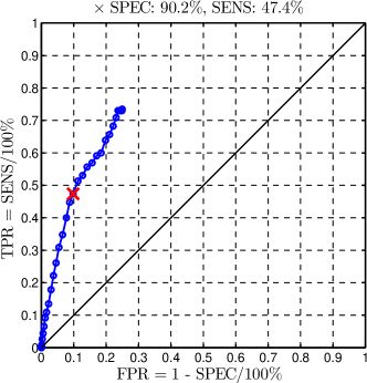
(a)
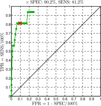
(b)

Figure 9: ROC curves for the binary classifier (29): (a) per frame basis, (b) per polyp basis. Red $\times$ mark the points corresponding to $R_{P}=37$. No-discrimination lines are solid black.

TABLE II: Numbers $N_{F}^{(p)}$, $p=1,\ldots,N_{S}$ of frames in each of $N_{S}=16$ sequences of “polyp” frames. Flags $D^{(p)}$, $p=1,\ldots,N_{S}$ indicating if at least one frame in the corresponding sequence was classified as “polyp”. Per polyp sensitivity for $R_{P}=37$ is $(13/16)\cdot 100\%=81.25\%$.

$N_{F}^{(p)}$	18	57	10	7	11	11	2	3	17	32	12	15	4	7	9	15
$D^{(p)}$	$\checkmark$	$\checkmark$	$\checkmark$	$\checkmark$	$\times$	$\checkmark$	$\checkmark$	$\checkmark$	$\checkmark$	$\checkmark$	$\times$	$\times$	$\checkmark$	$\checkmark$	$\checkmark$	$\checkmark$

We begin with a per frame ROC curve study, as described in section IV-B. The ROC curve for the binary classifier (29) is shown in Figure 9 (a). Note that it does not go all the way to $(1,1)$. The reason for that is the use of pre-selection and combined geometric criteria in steps 2 and 4 of Algorithm 1 respectively. For the frames that do not satisfy those criteria we set $R_{max}=0$, but for plotting the ROC curve we only use positive $R_{P}$. However, this limitation is not important, since the portion of the ROC curve that is of most interest to us is the one corresponding to the small values of $FPR$. This is due to the fact that an overwhelming majority of the frames in the endoscopy video sequences are non-polyp frames (all of them for healthy patients). The frames that the algorithm labels as “polyp” have to be inspected manually by a doctor. Thus, to minimize the work that the doctor has to do, the specificity has to be high.

According to our testing methodology, we set a target specificity at $90\%$. This specificity is achieved on a training subset with a decision threshold value of $R_{P}=37$ resulting in the specificity of $91\%$. When the binary classifier is applied to the whole data set with this threshold value, we obtain the specificity of $90.2\%$ and the sensitivity of $47.4\%$, which in shown in Figure 9 (a). This is a good performance, especially considering the fact that it is achieved on a relatively diverse data set. Moreover, such level of sensitivity for single frames can actually imply even better performance for video sequences, which is a more relevant way of evaluating the usefulness of the algorithm in the real clinical setting, as explained in section IV-B.

For a per polyp study we first show the values of the detection flags $D^{(p)}$ in Table II for all $N_{S}=16$ polyp frame sequences. These values are obtained for the value of the discrimination threshold $R_{P}=37$ as computed above. However, the sensitivity per polyp in this case is $81.25\%$, i.e. the algorithm correctly detects $13$ out of $16$ polyps in at least one frame of each corresponding sequence. Thus, as expected, the algorithm has a much better performance when a single polyp is present in a number of consecutive frames. This is further confirmed by Figure 9 (b), where we show a per polyp ROC curve. In fact, we observe that we can obtain a specificity of $93.47\%$, while sill maintaining the same per polyp sensitivity of $81.25\%$ if we take $R_{P}=40$.

By fixing the specificity at a high enough level we maintain control on how many frames are to be inspected manually. An important measure that allows us to assess the burden of such manual inspection in real clinical practice is the number of false positives and the false positive rate per patient. We display these values in Table III for each of the five patients that our data comes from. In all cases we observe a massive reduction in the amount of frames that need to be inspected manually. For example, the training subset of our data set corresponding to Patient $4$ ($8567$ non-polyp frames) is reduced to only $767$ frames that need to be inspected by a doctor.

TABLE III: False positives per patient. For each of five patients the number of normal (non-polyp) frames in the data set ($N_{norm}$), the number of false positives ($FPN$) and the false positive rate ($FPR$) are presented.

Patient	$N_{norm}$	$FPN$	$FPR$
1	422	34	8.0%
2	1008	55	5.4%
3	4666	671	14.3%
4	8567	767	8.9%
5	4075	310	7.6%
Total	18738	1837	9.8%

V-B Robustness

TABLE IV: Robustness study for Algorithm 1 with respect to the changes in the parameters. All values are given in percent. The base values $SPEC_{base}$, $SENS_{base}$ are in the “Base” row, the perturbed values $SPEC_{pert}$, $SENS_{pert}$ are in the rows below along with the sensitivities $\delta(SPEC)$, $\delta(SENS)$, with each row corresponding to a perturbation of a parameter indicated in the leftmost column.

	$SPEC$	$\delta(SPEC)$	$SENS$	$\delta(SENS)$	$SENS$	$\delta(SENS)$
			per frame	per frame	per polyp	per polyp
Base	92.2	–	47.4	–	81.2	–
$\sigma_{1}$	92.7	0.54	44.8	5.49	81.2	0
$\sigma_{2}$	90.5	1.84	53.5	12.87	93.8	15.5
$M_{L}$	92.3	0.11	47.0	0.84	81.2	0
$M_{U}$	91.8	0.43	49.6	4.64	81.2	0
$S_{L}$	92.2	0	47.4	0	81.2	0
$S_{U}$	92.0	0.22	48.3	1.90	81.2	0
$E_{max}$	91.7	0.54	48.7	2.74	81.2	0

To assess the robustness of Algorithm 1 with respect to the changes in the numerical parameters, we perform the sensitivity calculations as described in section IV-C. The results of the sensitivity calculations are given in Table IV. We observe that the algorithm is very robust with respect to all parameters, with a possible slight exception of $\sigma_{2}$. For a $10\%$ relative perturbation of the parameters the sensitivity of $SPEC$ is less than $1\%$ for all cases except $\sigma_{2}$, for which it is $1.8\%$. The sensitivity of per frame $SENS$ is larger, but still it is around $5\%$ or below for all parameters except for $\sigma_{2}$. The per polyp $SENS$ is even more robust. The $10\%$ parameter perturbation does not affect it at all with a same single exception. This is a remarkable display of robustness, considering that the algorithm is a highly non-linear procedure with lots of conditional branching based on thresholds.

The behavior in the single exceptional case (sensitivity with respect to $\sigma_{2}$) can be explained by the fact that $\sigma_{2}$ directly affects the maximal size of features in the mid-pass filtered frame. Thus, the increase in $\sigma_{2}$ leads to the increase in $R_{max}$. Since Algorithm 1 identifies large values of $R_{max}$ with polyps, this should lead to increased $SENS$, which we observe in Table IV for both per frame ($53.5\%$ perturbed against $47.4\%$ base) and per polyp ($93.8\%$ perturbed against $81.2\%$ base) basis. Even then, the relative sensitivity remains comparable with the size of the relative perturbation in $\sigma_{2}$ ($12.8\%$ per frame, $15.5\%$ per polyp against $10\%$).

VI Discussion

In this paper we developed an algorithm for automated detection of polyps in the images captured by a capsule endoscope. The problem of polyp detection is quite challenging due to a multitude of factors. These include the presence of trash liquids and bubbles, vignetting due to the use of a non-uniform light source, high variability of possible polyp shapes and the lack of a clear cut between the geometry of the polyps and the folds of a healthy mucosal tissue. We attempt to overcome these issues by utilizing both the texture information and the geometrical information present in the frame to obtain a binary classification algorithm with pre-selection.

We perform a thorough statistical testing of the algorithm on a rich data set to ensure its good performance in realistic conditions. The algorithm demonstrates high per polyp sensitivity and, equally importantly, displays a high per patient specificity, i.e. a consistently low false positive rate per individual patient. Such behavior is desirable as one of the main goals of automated polyp detection is to drastically decrease the amount of video frames that require manual inspection. While our approach is by no means an ultimate solution of the automated polyp detection problem, the achieved performance makes this work an important step towards a fully automated polyp detection procedure.

Throughout the paper we identified some directions of future research and the possible areas of improvement of the algorithm. We summarize them in the list below.

• Currently, the frame is converted to grayscale before processing, so the algorithm only utilizes the information about the texture and the geometry. It would be beneficial to also utilize the color information present in the frame. For example, the amount of red color can point to polyps that are highly vascularized.

• The effectiveness of our algorithm lies partially in the use of a pre-selection criterion. It is based on an idea of filtering out the non-informative frames without any further consideration. While using the texture content is a simple and robust procedure, more complicated pre-selection approaches can be used, e.g. from [23, 27]. In particular, in [27] the use of a Discrete Fourier Transform is proposed for frame classification as informative/non-informative. Another procedure from [27] that can be used to improve our pre-selection criterion is the specular reflection detection. It should be particularly effective in filtering out the frames with bubbles, since those typically produce strong specular reflections.

• The algorithm relies on a number of parameters. For the purpose of this study the values of most parameters were chosen manually. While the sensitivity computations in section IV-C demonstrate the robustness of the algorithm with respect to the changes in the parameter values, one may use an automated calibration procedure to choose these parameters. Developing such a procedure remains a topic of future research.

• A binary classifier for polyp detection is straightforward to implement and its performance can be easily assessed with the help of ROC curves. However, using more advanced machine learning and classification techniques may improve the detection of polyps. For example, support vector machines [7] were used in a polyp detection method based on a segmentation approach [6]. Alternatively, one can use a random forest [2, 15] to construct a classifier.

• In order to properly assess the size and shape of the protrusions, the algorithm should be able to correctly infer the actual height map of the object from the intensity information in the image. This presents a particular challenge when an object of interest is located in the dark section of the image. Using the mid-pass filtering provides an adequate solution to inferring the height map from the image. Nevertheless, we would like to investigate possible alternatives to the approach used here.

• Even if an algorithm perfectly detects polyp frames in a video sequence, it does not detect the actual location of a polyp in a colon. This problem is particularly exacerbated in capsule colonoscopy due to the highly irregular motion of the capsule. One way to overcome this issue is to try to reconstruct the capsule’s motion from the changes in the subsequent video frames. Alternatively, one may employ the approaches used in conventional colonoscopy. For example, in [22] a procedure is proposed for co-alignment of the optical colonoscopy video with a virtual colonoscopy from an X-ray CT exam. Tracking the movement of a capsule remains a topic of our research, whether by combining with other imaging modalities or by extracting the motion information directly from the video sequence.

References

- [1] D. G. Adler and C. J. Gostout, Wireless capsule endoscopy, Hospital Physician, 39 (2003), pp. 14–22.
- [2] L. Breiman, Random forests, Machine Learning, 45 (2001), pp. 5–32.
- [3] A. Buades, T. Le, J.-M. Morel, and L. Vese, Cartoon+Texture Image Decomposition, Image Processing On Line, 2011 (2011). http://dx.doi.org/10.5201/ipol.2011.blmv_ct.
- [4] Y. Cao, D. Li, W. Tavanapong, J. Oh, J. Wong, and P. C. de Groen, Parsing and browsing tools for colonoscopy videos, in Proceedings of the 12th annual ACM international conference on Multimedia, ACM, 2004, pp. 844–851.
- [5] Y. Cao, D. Liu, W. Tavanapong, J. Wong, J. H. Oh, and P. C. de Groen, Computer-aided detection of diagnostic and therapeutic operations in colonoscopy videos, Biomedical Engineering, IEEE Transactions on, 54 (2007), pp. 1268–1279.
- [6] F. Condessa and J. Bioucas-Dias, Segmentation and detection of colorectal polyps using local polynomial approximation, in Image Analysis and Recognition, Springer, 2012, pp. 188–197.
- [7] C. Cortes and V. Vapnik, Support-vector networks, Machine Learning, 20 (1995), pp. 273–297.
- [8] M. Delvaux and G. Gay, Capsule endoscopy: technique and indications, Best Practice & Research Clinical Gastroenterology, 22 (2008), pp. 813–837.
- [9] R. Eliakim, Video capsule colonoscopy: where will we be in 2015?, Gastroenterology, 139 (2010), p. 1468.
- [10] R. Eliakim, K. Yassin, Y. Niv, Y. Metzger, J. Lachter, E. Gal, B. Sapoznikov, F. Konikoff, G. Leichtmann, Z. Fireman, Y. Kopelman, and S. Adler, Prospective multicenter performance evaluation of the second-generation colon capsule compared with colonoscopy, Endoscopy, 41 (2009), pp. 1026–1031.
- [11] P. Figueiredo, I. Figueiredo, S. Prasath, and R. Tsai, Automatic Polyp Detection in Pillcam Colon 2 Capsule Images and Videos: Preliminary Feasibility Report, Diagnostic and Therapeutic Endoscopy, 2011 (2011), p. 182435.
- [12] J. Gerber, A. Bergwerk, and D. Fleischer, A capsule endoscopy guide for the practicing clinician: technology and troubleshooting, Gastrointestinal endoscopy, 66 (2007), pp. 1188–1195.
- [13] B. Gustafsson, H.-O. Kreiss, and J. Oliger, Time dependent problems and difference methods, Pure and Applied Mathematics (New York), John Wiley & Sons Inc., New York, 1995. A Wiley-Interscience Publication.
- [14] R. M. Haralick and L. G. Shapiro, Computer and Robot Vision, Volume I, Addison Wesley, 1992, pp. 28–48.
- [15] T. K. Ho, The random subspace method for constructing decision forests, Pattern Analysis and Machine Intelligence, IEEE Transactions on, 20 (1998), pp. 832–844.
- [16] R. S. Hunter, Photoelectric color difference meter, JOSA, 48 (1958), pp. 985–993.
- [17] G. Iddan, G. Meron, A. Glukhovsky, and P. Swain, Wireless capsule endoscopy, Nature, 405 (2000), p. 417.
- [18] A. Jemal, F. Bray, M. M. Center, J. Ferlay, E. Ward, and D. Forman, Global cancer statistics, CA: a cancer journal for clinicians, 61 (2011), pp. 69–90.
- [19] G. Kiss, J. Van Cleynenbreugel, S. Drisis, D. Bielen, G. Marchal, and P. Suetens, Computer aided detection for low-dose ct colonography, in Medical Image Computing and Computer-Assisted Intervention–MICCAI 2005, Springer, 2005, pp. 859–867.
- [20] M. Liedlgruber and A. Uhl, Computer-aided decision support systems for endoscopy in the gastrointestinal tract: A review, Biomedical Engineering, IEEE Reviews in, 4 (2011), pp. 73–88.
- [21] T. Lindeberg, Scale-space theory in computer vision, Springer, 1993.
- [22] J. Liu, K. R. Subramanian, and T. S. Yoo, An optical flow approach to tracking colonoscopy video, Computerized Medical Imaging and Graphics, 37 (2013), pp. 207–223.
- [23] , A robust method to track colonoscopy videos with non-informative images, International journal of computer assisted radiology and surgery, (2013), pp. 1–18.
- [24] A. Moglia, A. Menciassi, and P. Dario, Recent patents on wireless capsule endoscopy, Recent Patents on Biomedical Engineering, 1 (2008), pp. 24–33.
- [25] A. Moglia, A. Menciassi, P. Dario, and A. Cuschieri, Capsule endoscopy: progress update and challenges ahead, Nature Reviews Gastroenterology and Hepatology, 6 (2009), pp. 353–361.
- [26] T. Nakamura and A. Terano, Capsule endoscopy: past, present, and future, Journal of gastroenterology, 43 (2008), pp. 93–99.
- [27] J. Oh, S. Hwang, J. Lee, W. Tavanapong, J. Wong, and P. C. de Groen, Informative frame classification for endoscopy video, Medical Image Analysis, 11 (2007), pp. 110–127.
- [28] M. Pauly, Point primitives for interactive modeling and processing of 3D geometry, Hartung-Gorre, 2003.
- [29] C. Spada, C. Hassan, R. Marmo, L. Petruzziello, M. E. Riccioni, A. Zullo, P. Cesaro, J. Pilz, and G. Costamagna, Meta-analysis shows colon capsule endoscopy is effective in detecting colorectal polyps, Clinical Gastroenterology and Hepatology, 8 (2010), pp. 516–522.
- [30] R. M. Summers, C. D. Johnson, L. M. Pusanik, J. D. Malley, A. M. Youssef, and J. E. Reed, Automated polyp detection at ct colonography: Feasibility assessment in a human population1, Radiology, 219 (2001), pp. 51–59.
- [31] C. van Wijk, V. F. van Ravesteijn, F. M. Vos, and L. J. van Vliet, Detection and segmentation of colonic polyps on implicit isosurfaces by second principal curvature flow, Medical Imaging, IEEE Transactions on, 29 (2010), pp. 688–698.
- [32] J. Yao, M. Miller, M. Franaszek, and R. M. Summers, Colonic polyp segmentation in ct colonography-based on fuzzy clustering and deformable models, Medical Imaging, IEEE Transactions on, 23 (2004), pp. 1344–1352.
- [33] H. Yoshida and J. Nappi, Three-dimensional computer-aided diagnosis scheme for detection of colonic polyps, Medical Imaging, IEEE Transactions on, 20 (2001), pp. 1261–1274.
- [34] Y. Zheng, J. Yu, S. B. Kang, S. Lin, and C. Kambhamettu, Single-image vignetting correction using radial gradient symmetry, in IEEE Conference on Computer Vision and Pattern Recognition, IEEE, 2008, pp. 1–8.