Apsidal motion in massive close binary systems.
I. HD 165052 an extreme case?

Abstract

We present a new set of radial-velocity measurements of the spectroscopic binary HD 165052 obtained by disentangling of high-resolution optical spectra. The longitude of the periastron ($\varpi=60\pm 2$ degrees) shows a variation with respect to previous studies. We have determined the apsidal motion rate of the system $\dot{\varpi}=12.1\pm 0.3\degr$yr^-1, which was used to calculate the absolute masses of the binary components: $M_{1}=~{}22.5\pm 1.0~{}M_{\sun}$ and $M_{2}=20.5\pm 0.9~{}M_{\sun}$. Analysing the separated spectra we have re-classified the components as O7Vz and O7.5Vz stars.

1 Introduction

O-type stars are objects that deserve great astrophysical interest. Usually, they are located in star forming regions where, due to their high-velocity winds and intense UV radiation, they determine the dynamical and ionization state of the neighboring interstellar medium. The turbulence they generate in the interstellar medium drives galactic dynamos. Furthermore, their high luminosities dominate the radiation of their birth regions, open clusters, spiral arms and even entire galaxies. Besides, by mean of their explosive end as supernovae, they play a key role in the chemical evolution of the interstellar medium and therefore in the metal enrichment of the successive generations of stars. However, several features of O-type stars are still poorly known. Specially their masses represent a fundamental astrophysical parameter, which is still highly uncertain for various spectral sub-types. For this reason, to establish constraints to the masses of O-type stars is a very important task. The most direct and reliable method to determine stellar masses is the analysis of the Keplerian motion in detached double-lined eclipsing binary systems. The photometric and spectroscopic observation of such systems, and the subsequent analysis of the variations in their brightness and radial velocities (RV), allows to calculate the parameters of their orbital motion and the minimum masses of their components. Furthermore, the observation of eclipses indicates that the orbital plane lies close to the line of sight (i. e. its inclination $i$ is close to 90°). Then, using adequated models of stellar structure, it is possible to derive absolute stellar masses. However, it should be emphasized that this can be done only for a very limited number of systems, since the constraint $i\sim 90$° is quite strong.

In close binaries, due to the proximity of the companion the stars are no longer spherical. This leads to the occurrence of finite quadrupolar, and higher, momenta of the gravitational field (cf. Sterne 1939). These momenta force eccentric orbits to precess –i.e. modifies the position of the periastron (apside or apse)–. Additionally, General Relativity predicts a secular apsidal motion, which is independent of the classical contributions, but it is related again with the components masses (cf. Levi-Civita 1937). It has been shown that the knowledge of the apsidal motion rate (AMR) allows to estimate absolute masses in massive close binary systems with unknown orbital inclination even in the case of non-eclipsing binaries (Benvenuto et al., 2002, B02). From a theoretical point of view, the AMR is strongly dependent on the radii and internal structure of the stars of the pair. So, the masses determined by this method will be model dependent. In any case, accurate RV measurements and improved stellar evolutionary models make currently feasible its use in reliable mass determinations. In order to increase the number of O-type stars with determined absolute masses we are conducting a systematic high-resolution spectroscopic monitoring of binary systems with eccentric orbits with the aim of calculating their masses taking advantage of this method.

One of the objects that we are studying is HD 165052 (= CD -24 13864; $\alpha_{2000}=18^{h}05^{m}10.6^{s}$, $\delta_{2000}=-24$°23’55”; $V=6.87$) an O-type double-lined spectroscopic binary star member of the open cluster NGC 6530 in the H ii region M8 (the Lagoon Nebula). It was first catalogued in the Cordoba Durchmusterung by Thome (1892). Plaskett (1924) discovered variations in the RV of this star, while double lines in its spectrum were first noticed by Conti (1974). Morrison & Conti (1978) presented the first orbital solution for the system (see Table 3). An improved circular orbital solution was calculated by Stickland, Lloyd, & Koch (1997, S97) adding RV measurements from IUE spectra. A few years later, Arias et al. (2002, A02) analysed high-resolution optical spectra, and determined a slightly eccentric ($e=0.09$) orbital solution. They fitted the previous RV data with their own solution and found evidence of apsidal motion. Linder et al. (2007, L07) determined a new orbital solution for the system which agrees with the A02 one.

In order to establish (or rule out) the AMR in HD 165052 we have systematically observed this star between 2008 and 2010, and gathered a set of high-resolution spectra (see Sec. 2). Using the technique of disentangling (cf. González & Levato 2006) we have measured the RVs and simultaneously obtained separated spectra of the two components of the binary (see Sec. 3.1). This procedure allowed us to re-classify the spectra of both components (Sec. 3.2) and to fit a new orbital solution (Sec. 3.4). We have confirmed the existence of apsidal motion and measured the AMR for the first time (Sec. 3.5). Then, applying the method mentioned above (B02) we have calculated the masses of the system components (Sec. 3.6).

2 Observations

We have acquired 37 high-resolution spectra of HD 165052 (see journal of observations on Table 2): 29 at CASLEO, Argentina, with the 2.15-m Jorge Sahade telescope between 2008 August and 2010 August using the REOSC SEL Cassegrain spectrograph in cross-dispersion mode; 5 at Las Campanas Observatory (LCO), Chile, with the Irénée du Pont 2.5-m telescope using the Echelle Spectrograph in May 2010; and 3 additional spectra using FEROS at ESO La Silla, Chile, with the 2.2-m telescope in 2009 May. The spectra taken at LCO and ESO La Silla belong to the “OWN Survey” program (Barbá et al., 2010). The mean signal to noise ratio (SNR) of all these spectra is $\sim 200$. Technical details of the instrumental configurations can be found in Table 1. All the spectra were reduced using the standard routines of IRAF.

Table 1: Technical characteristics of the instruments in the configurations used for this work.

Telescope - instrument	reciprocal	R	spectral
	dispersion	@5000Å	range
	(Å/pixel)		(Å)
CASLEO-J.S.-REOSC	0.19	13000	3600 - 6100
ESO-2.2-FEROS	0.03	45000	3600 - 9200
LCO-du Pont-Echelle	0.05	35000	3500 - 10100

At CASLEO every night we have taken at least one spectrum of the star HD 137066, a RV standard established using CORAVEL photoelectric scanner by Andersen et al. (1985) with $v_{r}=-8.72\pm 0.15$ km s^-1. We have also observed the B0V star $\tau$ Sco, considered as a rotational velocity standard in the Slettebak et al. (1975) system with $v\sin i<10$ km s^-1. The latter spectra were taken with the same instrumental configuration as those of HD 165052 and averaged to achieve a SNR $\ga 600$ in the region of interest.

Spectra from CASLEO and LCO were calibrated using comparison spectra taken after every single exposition from a Th-Ar lamp.

3 Results and discussion

3.1 Disentangling and radial velocity measurements

In order to measure the RVs, we applied the disentangling method described by González & Levato (2006) which allows to separate simultaneously the spectra of the binary components. This iterative procedure consists in using alternatively the spectrum of one component to calculate the spectrum of the other one. In each step, the spectrum of one star is used to subtract its spectral features from the composite one. Then, the RVs are measured in the resulting single-lined spectra. This spectra are shifted appropriately and combined to compute the new spectrum of each component.

We have started the iterations using a template spectrum of the secondary star taken from the grid of stellar atmosphere models in the TLUSTY database (Lanz & Hubeny, 2003) with solar metallicity, $T_{\mathrm{eff},2}=35000$K and a $\log{g}_{2}=4.0$ that corresponds to main sequence star (cf. Sec. 3.2). The $T_{\mathrm{eff}}$ was chosen adopting the spectral type calibration of Martins, Schaerer, & Hillier (2005). The template was convolved to the projected rotational velocity estimated by Morrison & Conti (1978). As it has been shown by González & Levato (2006) these initial guesses do not affect the final results.

The method also requires a RV initial value for each spectrum. A first raw measurement of the central wavelengths of the spectral lines He i $\lambda\lambda$ 4471, 4921, 5876, He ii $\lambda\lambda$ 4686 and 5411 was made using splot task of IRAF. The RVs calculated from these lines were averaged to obtain a first estimate of the RV of each component. Instead, during disentangling iterations the cross-correlation function was calculated over a disjoint sample region composed by 17 wavelengths intervals, each $\sim$10 Å wide, taken around the following spectral lines: He i $\lambda\lambda$ 3819, 4026, 4387, 4471, 4713, 4921, 5015, 5875, He ii $\lambda\lambda$ 4200, 4542, 4686, 5411, C iv $\lambda\lambda$ 5801, 5812, O iii $\lambda$ 5592, Mg ii $\lambda$ 4481 and Si iv $\lambda$ 4088. The RVs thereby measured are listed in Table 2 and reproduced as mean RVs in the Table 2.

In order to provide detailed data for future works, we have subsequently defined several sampling regions, each one around a single spectral line, and compute the cross-correlation separately for each region. So we have measured the RVs of the individual lines listed in Table 2. The spectral lines selected were the same of A02 to allow for a comparison with that work. As it can be seen in Appendix B.2, the overall behavior of the RVs of the individual lines agrees with that of the mean RV.

Table 2: Journal of the observations of HD 165052. Radial velocity measurements used to compute the orbital solution given in Table 3.

HJD	phase	$v_{1}$	O-C	$v_{2}$	O-C	Obs.
$-2450000$	$\phi$
4582.8675	0.90	97.1	-2.6	-108.8	-2.4	CAS
4693.6231	0.38	-81.6	3.2	91.7	-3.9	CAS
4695.6483	0.06	13.8	0.9	-8.8	2.6	CAS*
4696.5568	0.37	-85.4	0.8	95.1	-1.9	CAS
4696.6286	0.39	-80.2	0.9	94.3	2.8	CAS
4696.6605	0.40	-76.8	1.6	91.4	2.8	CAS
4697.6220	0.73	73.7	2.9	-76.1	-1.4	CAS
4955.8004	0.10	-7.6	5.3	5.1	-11.7	ESO*
4956.9100	0.47	-57.5	-2.4	61.0	-2.0	ESO
4964.8865	0.17	-57.6	0.5	66.7	0.4	CAS
4965.8323	0.49	-47.1	0.0	57.4	3.2	CAS
4966.8550	0.84	100.8	-1.4	-106.1	2.9	CAS
4967.8220	0.16	-56.1	-1.3	62.9	0.2	CAS
4968.8723	0.52	-38.8	-4.6	40.5	0.5	CAS
5046.6533	0.84	103.7	1.3	-109.9	-0.5	CAS
5047.7305	0.21	-73.8	-0.7	81.8	-1.0	CAS
5048.7185	0.54	-24.6	-0.2	29.3	-0.2	CAS*
5049.7159	0.88	106.4	4.3	-106.5	2.5	CAS
5052.7320	0.90	100.6	1.5	-104.9	0.8	CAS
5337.6475	0.31	-94.3	-2.8	101.3	-1.6	LCO
5339.7307	0.02	38.0	-3.8	-45.7	-2.7	LCO
5340.6327	0.33	-94.6	-3.4	100.7	-1.8	LCO
5341.5812	0.65	26.4	-3.8	-27.4	2.9	LCO*
5342.6292	0.00	54.0	-0.5	-60.9	-4.0	LCO
5376.5522	0.48	-52.2	-0.3	59.9	0.4	CAS
5378.7551	0.23	-79.7	0.0	88.5	-1.4	CAS
5380.5253	0.82	97.3	-3.3	-106.1	1.2	CAS
5381.7473	0.24	-84.7	-1.7	93.2	-0.4	CAS
5383.7515	0.92	91.5	-3.2	-98.5	2.5	CAS
5429.6974	0.46	-57.0	1.1	70.1	3.8	CAS
5430.6168	0.78	87.8	-1.1	-91.7	2.9	CAS
5431.6959	0.14	-42.6	-1.1	51.4	3.2	CAS
5432.6362	0.46	-58.1	2.1	69.5	0.9	CAS
5433.5059	0.75	81.0	0.0	-88.3	-2.4	CAS
5434.6834	0.15	-46.7	1.2	61.2	6.1	CAS
5435.5627	0.45	-65.0	-1.2	74.0	1.4	CAS
5698.8397	0.54	-6.0	17.1	41.2	13.2	ESO*

Velocities and O-C in km s^-1. *: one tenth weight assigned in orbital solution fit because of strong lines blending. Obs.: observatory where the spectrum was acquired. CAS: CASLEO; ESO: ESO La Silla; LCO: Las Campanas.

3.2 Spectral analysis

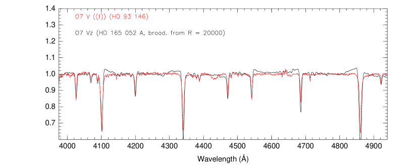
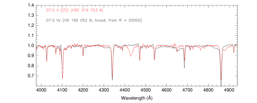
Figure 6: HD 165052 primary (A) and secondary (B) star spectra resample to $R\sim 2500$ (black) compared with that of the spectral standards HD 93146 and HDE 319703 A (red). It could be note the greater intensity of He ii $\lambda$ 4686 absorption line (the z feature). The difference between the continuum level at bluer and redder wing of some lines is due to an artefact of the disentangling algorithm. Figures generated with MGB code (Sota et al., 2011).

We have visually compared our disentangled spectra with those of the atlas of spectral standards published by Sota et al. (2011) using the MGB code (Maíz Apellániz et al., 2011). We have observed in both components that the intensity of the absorption line He ii $\lambda$ 4686 is greater than both He i $\lambda$ 4471 and He ii $\lambda$ 4542 (see Fig. 6), a fact that is noted with a z qualifier of the spectral type (cf. Walborn 2009). Thus we classified the primary as O7Vz and the secondary as O7.5Vz.

In the past, other authors have classified these stars spectroscopically. Morrison & Conti (1978) observed that both stars are normal, with no conspicuous mass loss, and not far from the ZAMS. A02 showed that spectral types are O6.5V for the primary component and O7.5V for secondary. L07 concluded that the system could be a O6.5V + O7V, or O6.5V + O7.5V, perhaps O((f)) because they detected N iii $\lambda\lambda$ 4634, 40 and 41 in emission. We see some traces of a very weak emission around 4640 in a couple of FEROS spectra. In our disentangled primary-component spectrum, the absorption lines He i $\lambda$ 4471 and He ii $\lambda$ 4542 seems to have almost the same intensity. That is why we suspect it could be an O7V rather than an O6.5V star. For the classification of the secondary, we agree with the spectral type proposed by A02 and L07.

3.3 Projected rotational velocity

One of the stellar parameters required to mass determination is the projected rotational velocity $v\sin i$ of the binary components, since it is used to compute the internal structure constants (see Sec. 3.6).

To estimate the $v\sin i$, the spectrum of $\tau$ Sco has been convolved with rotation line profiles calculated for different projected rotational velocities. The He i $\lambda\lambda$ 4713 and 5015 absorption lines were selected for these measurements because they are isolated in the spectra and their Stark broadening can be considered as negligible (cf. Dimitrijevic & Sahal-Brechot 1990). The full width at half maximum of intensity (FWHM) of these lines in the convolved spectra of $\tau$ Sco were measured and a linear relation between FWHM and the $v\sin i$ was fitted supposing a rotational velocity very lower than the critical one (cf. Collins 1974). Specifically it was found $FW\!H\!M_{4713}=0.0228\times v\sin i+0.219$ and $FW\!H\!M_{5015}=0.0239\times v\sin i+0.277$ Å, into the interval $30\leq v\sin i\leq 100$ km s^-1. These empirical regressions were used to convert the FWHM of each line measured in the disentangled spectra in a $v\sin i$ value.

Thereby we have computed $v_{1}\sin i=71\pm 5$ km s^-1 and $v_{2}\sin i=66\pm 5$ km s^-1. Where the errors were estimated as half the uncertainty in the projected rotational velocity of $\tau$ Sco.

Other authors have estimated the $v\sin i$ of these stars, i.e. from IUE spectra, S97 have found $v_{1}\sin i$ = 85$\pm$8 and $v_{2}\sin i=80\pm 6$ km s^-1; Morrison & Conti (1978) have obtained from the FWHM intensity of the individual profiles of He i $\lambda$ 4471, $v_{1}\sin i=65\pm 9$ and $v_{2}\sin i=69\pm 4$ km s^-1; and L07 determined $v_{1}\sin i=73\pm 7$ and $v_{2}\sin i=80\pm 7$ km s^-1 using the profiles of the disentangled lines He ii $\lambda$ 4471, He ii $\lambda$ 4542 and H$\beta$. From the four independent determinations, it is clear that the projected rotation velocity of both stars is very similar (within errors). Our results compare better with the later ones.

3.4 Orbital solution

Our orbital solution was obtained using the RVs given in Table 2 as input for the GBART code. The orbital parameters determined from the best-fitting are shown in the last column of Table 3 and depicted in Figure 1. Our new orbital solution is close to the already published ones by S97, A02 and L07. The latter discussed about the comparison among them. We also found a non-negligible eccentricity, thus confirming its reliability. However, we point out the noticeable difference among the periastron longitudes ($\varpi$), a clear sign of apsidal motion, which will be analysed in the following.

Table 3: Orbital solutions previously published for HD 165052 to be compared with this work.

Element	M78	S97	A02	L07	this work
$P$ (days)	$6.140\pm 0.002$	2.955055	$2.95510\pm 0.00001$	$2.95515\pm 0.00004$	$2.95506\pm 0.00002$
$e$	$0.064\pm 0.041$	0.0 (assumed)	$0.09\pm 0.004$	$0.081\pm 0.015$	$0.090\pm 0.003$
$\varpi$(°)	$304\pm 56$ (†)	undefined	$296.7\pm 3.5$	$298.0\pm 10.2$	$60\pm 2$
$T_{0}$	$42939.5\pm 0.6$	$49819.075\pm 0.008$	$49871.75\pm 0.03$	$51299.053\pm 0.081$	$55050.08\pm 0.02$
(HJD-2400000)
$TV_{max}$			$49872.19\pm 0.03$		$55049.66\pm 0.02$
(HJD-2400000)
$V_{0}$ (km s-1)	$3.0\pm 4.6$	$-0.9\pm 1.3$	$1.05\pm 0.31$	$2.1\pm 1.2$*	$1.3\pm 0.2$
$K_{1}$ (km s-1)	$91.0\pm 2.8$	$95.6\pm 2.2$	$94.8\pm 0.5$	$96.4\pm 1.6$	$97.4\pm 0.4$
$K_{2}$ (km s-1)	$104.0\pm 8.6$	$109.6\pm 2.2$	$104.7\pm 0.5$	$113.5\pm 1.9$	$106.5\pm 0.4$
$a_{1}\sin i$ ($R_{\odot}$)	$11.1\pm 0.3$	$5.58\pm 0.13$	$5.51\pm 0.03$	$5.6\pm 0.1$	$5.66\pm 0.03$
$a_{2}\sin i$ ($R_{\odot}$)	$12.7\pm 0.7$	$6.40\pm 0.13$	$6.09\pm 0.03$	$6.6\pm 0.1$	$6.20\pm 0.03$
$M_{1}\sin^{3}i$ ($M_{\odot}$)	$2.5\pm 0.5$	$1.41\pm 0.07$	$1.26\pm 0.03$	$1.5\pm 0.1$	$1.34\pm 0.03$
$M_{2}\sin^{3}i$ ($M_{\odot}$)	$2.2\pm 0.3$	$2.23\pm 0.06$(††)	$1.14\pm 0.03$	$1.3\pm 0.1$	$1.22\pm 0.03$
$q(M_{2}/M_{1})$	$0.87\pm 0.08$	$0.87\pm 0.03$	$0.90\pm 0.01$	$0.85\pm 0.01$	$0.91\pm 0.01$
r.m.s. (km s-1)		7.4	2.21	6.2	1.7

M78: Morrison & Conti (1978); S97: Stickland, Lloyd, & Koch (1997); A02: Arias et al. (2002); L07: Linder et al. (2007). (†): measured from maximum positive radial velocity of star 1. (††): it seems that there was a typing mistake in this paper. The mass should probably be 1.23 $M_{\sun}$. *: L07 fitted considering possible different systemic velocities for both components. Listed value corresponds to primary. For secondary they found $1.4\pm 1.3$ km s^-1.

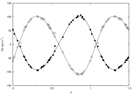
Figure 1: Radial-velocity curve of HD 165052 calculated with the ephemerids of the orbital solution found in this work (Table 3). Measurements from Table 2 are also represented (filled circles: primary radial velocities; open: secondary). $\phi$ = 0 corresponds to the periastron passage.

3.5 Apsidal motion

Our orbital solution (Table 2) gives $\varpi=60\pm 2\degr$, a very different value than those found by A02 and L07 –two solutions based on observations overlapped in time–. We consider that this variation confirms the existence of apsidal motion in the system. To determine its rate, we have re-computed orbital solutions, fixing $P=2.95506$ days and $e=0.090$ (note that our values for these parameters do not differ significantly from those of S97, A02 and L07), to the previously published RVs. To do it we have grouped those data in four data sets according to the proximity of its observation date (see Table 4). It means we have joined together the data from A02 and L07, while we have not taken into account 4 data points from S97 between HJD 2444121.777 and 2445123.793. It is worth note that the zero point in RV does not vary, within errors, between the different datasets. We have considered each $\varpi_{\mathrm{i}}$ thus obtained as representative of the longitude of the periastron at an epoch $t_{\mathrm{i}}$ equal to the mid-point time between the first and the last date of the observations in those particular dataset. Since the variation of $\varpi$ in time seems to have a linear trend (see Fig. 2) we have computed a linear regression, which slope was considered as a first approximation to the AMR of the system:

$$\dot{\varpi}=0.0322\pm 0.0005\degr\mathrm{day}^{-1}.$$ (1)

We have also used the FOTEL code developed by Hadrava (2004), which allows to solve a RV curve taking into account the apsidal motion. We have applied FOTEL to all the available RV (Table 6) using as initial values our set of orbital parameters (Table 3, col. “this work”) and the $\dot{\varpi}$ value just found. Permitting the code to fit all the parameters simultaneously, the fitting process converged to a set of orbital elements which agrees, within errors, with the values determined using the individual datasets. The AMR thus obtained was

$$\dot{\varpi}=0.0340\pm 0.0007\degr\mathrm{day}^{-1}.$$ (2)

Table 4: Longitude of the periastron $\varpi$ and others orbital elements at different epochs re-computed from previously published RVs measurements fixing $P=2.95506$ days and $e=0.090$.

Dataset no.:	1	2	3	4
initial date (HJD-2400000)	42560.940	48864.018	49854.6400	54582.8675
final date (HJD-2400000)	43092.571	49965.110	52383.8577	55698.8397
data from	M78	S97	A02, L07	this work
$\varpi$(°)	$27\pm 22$	$247\pm 9$	$293\pm 4$	$60\pm 2$
$V_{0}$ (km s-1)	$0\pm 2$	$-1.7\pm 0.9$	$1.3\pm 0.4$	$1.3\pm 0.2$
$K_{1}$ (km s-1)	$94\pm 4$	$97\pm 2$	$95.4\pm 0.8$	$97.4\pm 0.4$
$K_{2}$ (km s-1)	$103\pm 4$	$106\pm 2$	$107.8\pm 0.8$	$106.5\pm 0.4$
$q$	$0.91\pm 0.07$	$0.91\pm 0.03$	$0.89\pm 0.01$	$0.91\pm 0.01$
r.m.s. (km s-1)	8.4	3.2	4.1	1.7

References as in Table 3.

Figure 2: Variation of the longitude of the periastron ($\varpi$) in time. Horizontal error bars indicates the time span of each observational dataset. A linear fit with slope $0.0322\pm 0.0005$°day^-1 is shown (data from Table 4).

In the following calculations we have used for AMR the value

$$\dot{\varpi}=0.0331\pm 0.0009\degr\mathrm{day}^{-1},$$ (3)

since it is the mean between (1) and (2), while we have adopted as its error the semi-difference among them. (This AMR corresponds to $12.1\pm 0.3\degr$ yr^-1 or alternatively to an apsidal period $U=29.8\pm 0.8$ years). It seems to be the highest AMR ever measured in an O+O system, with the possible exception of DH Cep (HD 215835) whose AMR has still to be confirmed (cf. Petrova & Orlov 1999, Bulut & Demircan 2007 and ref. therein).

3.6 Calculation of the masses of the system employing the advance of the apside

As stated above (see Sec. 1), the measurement of the secular advancement of the apside allows for the determination of the masses of the components of the system even for the case of non-eclipsing binaries. The method to be employed below has been proposed and applied for the massive, non-eclipsing binary HD 93205 by B02 (see also Jeffery 1984).

As it is well known, the gravitational potential of each component of the pair is affected by the presence of the other star and also by its own rotation. If we consider only the lowest (quadrupolar) correction to the gravitational potential of each object, the theoretical advancement of the apside is given by the Eq. (14) of Sterne (1939):

$$\frac{\dot{\varpi}}{\Omega_{\mathrm{orbit}}}=k_{2,1}\bigg{(}\frac{a_{1}}{A}\bigg{)}^{5}\bigg{[}15\frac{M_{2}}{M_{1}}f_{2}(e)+\frac{\omega^{2}_{1}A^{3}}{GM_{1}}g_{2}(e)\bigg{]}+$$

$$k_{2,2}\bigg{(}\frac{a_{2}}{A}\bigg{)}^{5}\bigg{[}15\frac{M_{1}}{M_{2}}f_{2}(e)+\frac{\omega^{2}_{2}A^{3}}{GM_{2}}g_{2}(e)\bigg{]}.$$ (4)

Here $\dot{\varpi}$ is the AMR; $\Omega_{\mathrm{orbit}}$ denotes the mean orbital angular velocity; $k_{\mathrm{i,j}}$ are the internal structure constants for the $i$-th multipolar term of the potential expansion (here $i=2$) and $j$ denotes the component of the pair (see below for details); $G$ is the gravitational constant; $A$ is the semi axis of the relative orbit; $M_{\mathrm{i}}$, $a_{\mathrm{i}}$, $\omega_{\mathrm{i}}$ are the mass, mean radius and angular rotation velocity of the $i$-th star respectively. $f_{2}(e)$ and $g_{2}(e)$ are functions of the eccentricity $e$ given by

$$f_{2}(e)=\frac{1+\frac{3}{2}e^{2}+\frac{3}{8}e^{4}}{(1-e^{2})^{5}}$$ (5)

and

$$g_{2}(e)=\frac{1}{(1-e^{2})^{2}}.$$ (6)

The first and second terms of the r.h.s. of Eq. (4) correspond to the contributions due to the primary and secondary stars, respectively. In each of these terms, the first term in the bracket is due to the tidal effect of one star on the other while the second one is due to stellar rotation.

$$\frac{\dot{\varpi}_{\mathrm{GR}}}{\Omega_{\mathrm{orbit}}}=6.36\times 10^{-6}\frac{M_{1}+M_{2}}{A(1-e^{2})},$$ (7)

where masses and $A$ are in solar units. The internal structure constants $k_{\mathrm{i,j}}$ are dependent on the structure of the stars. Most stellar evolution codes assume spherical symmetry, ignoring rotation. However, the departure from sphericity due to rotation modifies $k_{\mathrm{i,j}}$ appreciably. Fortunately, Claret (1999) has shown that accounting for this correction is very simple, at least for $i=2$. If we define $[k_{2,\mathrm{j}}]_{\mathrm{sph}}$ as the internal structure constant corresponding to a spherical star, the corrected value of $k_{\mathrm{{i,j}}}$ is given by

$$\lg k_{2,\mathrm{j}}=\lg[k_{2,\mathrm{j}}]_{\mathrm{sph}}-0.87\frac{2V^{2}_{\mathrm{j}}}{3g_{\mathrm{j}}a_{\mathrm{j}}},$$ (8)

where $V_{\mathrm{j}}$ is the tangential velocity and $g_{\mathrm{j}}$ the surface gravitational acceleration. We shall consider

$$\frac{\dot{\varpi}}{\Omega_{\mathrm{orbit}}}+\frac{\dot{\varpi}_{\mathrm{GR}}}{\Omega_{\mathrm{orbit}}}=\frac{\dot{\varpi}_{\mathrm{obs}}}{\Omega_{\mathrm{orbit}}}$$ (9)

as an equation for $M_{1}$ as described in B02 where the reader will find further details on the method. As discussed there, this method is model dependent, because $k_{\mathrm{i,j}}$ evolves due to changes in the density profile of the star and, more importantly, $a_{\mathrm{j}}$ also evolves. Notice the steep dependence of Eq. (4) with the value of $a_{\mathrm{j}}$. Thus, as a matter of facts, this method is age dependent.

In order to apply the above described method, we consider that both stars have the same age and are still burning hydrogen on their cores as it is indicated by spectral classification. We have computed solar composition stellar models with masses from 15 $M_{\odot}$ to 40 $M_{\odot}$ during core hydrogen burning in steps of 0.5 $M_{\odot}$. These models include mass loss as in de Jager, Nieuwenhuijzen, & van der Hucht (1988) and overshooting as in Demarque et al. (2004) the rest of the code corresponds to that described by Benvenuto & De Vito (2003) for binary evolution.

We show, in Fig. 3 the Hertzsprung - Russell diagram for stellar masses in the range corresponding to the components of the pair with the evolutionary tracks calculated using these models. We set stellar ages to zero on the ZAMS.

Also, we have computed the coefficient $k_{2,\mathrm{j}}$ whose evolution, for different values of the initial mass is shown in Fig. 4 together with $k_{2,\mathrm{j}}(R/R_{\odot})^{5}$, which appears in Eq. (4). Now, we are in a position to employ the secular advancement of the apside ($\Omega_{\mathrm{apse}}\equiv\dot{\varpi}$) to determine the mass of the primary. A comparison of the theoretical results with observations is presented in Fig. (5). For a given age of the pair, the mass value of the primary corresponds to the intersection of the theoretical curve with the horizontal line at $\Omega_{\mathrm{apse}}/\Omega_{\mathrm{orbit}}=(2.72\pm 0.08)\times 10^{-4}$. The advancement of the apside is due to $\approx 74$, $\approx 23$ and $\approx 3$ per cent to tidal, rotational and relativistic contributions, respectively.

If we assume that the age of NGC 6530 is 1.5 Myr (see Sec. 3.7) the most probable mass value for the primary of HD 165052 is $22.5\pm 1.0~{}M_{\odot}$, where the error was estimated considering an age uncertainty of 0.5 Myr. Using the binary mass ratio $q$ from our orbital solution we found that the most probable value for the mass of the secondary is $M_{2}=20.5\pm 0.9~{}M_{\sun}$ .

Figure 3: Evolutionary tracks in the Hertzsprung - Russell diagram for stars of 20, 30, and 40 $M_{\odot}$ (solid lines) and 22, 24, 26, 28, 32, 34, 36 and 38 $M_{\odot}$ (dotted lines) during core hydrogen burning. On each track, filled dots indicate time intervals of 1 Myr. Crosses: location of binary components according to literature. Horizontal error bars: $T_{\mathrm{eff}}$ dispersion in Martins et al. (2005, Table 4) observational calibration. Vertical bars: lower limit: distance modulus from Mayne & Naylor (2008). Upper limit: $M_{V}$ from Buscombe (1969) (see details in Sec. 3.7). Circles: components derived from apsidal motion rate (filled primary); error bars depict the age uncertainty propagated to masses.

Figure 4: Temporal evolution of the coefficients $k_{2,\mathrm{j}}$ (solid lines) and $k_{2,\mathrm{j}}(R/R_{\odot})^{5}$ (dotted lines) for stars of 15, 20, 30, and 40 $M_{\odot}$. Curves end at larger ages the smaller is the mass. For further details see Sec. 3.6.

Figure 5: The secular advance of the apse as a function of the mass of the primary component of HD 165052 for different values of the age of the system, depicted in solid lines. The value corresponding to observations is denoted with an horizontal long dashed line. The value of the mass of the primary corresponds to the intersections: for ages of 0, 1, 2, 3, and 4 Myr the values for the mass of the primary are of $28.4\pm 0.7$, $23.5\pm 0.5$, $21.5\pm 0.4$, $19.6\pm 0.3$ and $18.1\pm 0.3M_{\sun}$ respectively. Evidently, the uncertainty in the age of the system has a direct impact on the determination of the masses of the components of the system.

As HD 165052 is a much closer pair than HD 93205, it is worth to analyse the possibility of considering contributions to the apsidal motion due to terms beyond the quadrupolar. These contributions have been given by Sterne (1939). It is found that the next term in the expansion for the advancement of the apside is approximately

$$2\frac{k_{3,\mathrm{j}}}{k_{2,\mathrm{j}}}\bigg{(}\frac{a_{\mathrm{j}}}{A}\bigg{)}^{2}$$

times the tidal term considered in Eq. (4). Considering the solution given by Eq. (9), we find that $a_{\mathrm{j}}/A\approx 1/3$ whereas the ratio of the internal structure constants can be estimated by employing the Table 15 of Claret & Gimenez (1991) corresponding to a stellar model of 25 $M_{\odot}$. It is found that $k_{3,\mathrm{j}}/k_{2,\mathrm{j}}\approx 1/3$. Thus, the correction due to the first term beyond the quadrupolar one is of the order of 4 per cent. This is far smaller than the uncertainty in the theoretical AMR due to an error of 0.5 Myr in the age of the pair. This fact justifies the employment of Eq. (4) up to the lowest order contribution.

The components masses that we have obtained are in agreement, within errors, with the spectroscopic masses derived by Martins et al. (2005) from a $T_{\mathrm{eff}}$ calibration of O stars. In fact, they obtained $25.3~{}M_{\sun}$ for an O7V star and $22.9~{}M_{\sun}$ for an O7.5V with an uncertainty as high as 35 to 50 per cent. On the other hand, the masses calculated are close to the range of masses most reliable determined via detached eclipsing binaries for these spectral types. For example, the O7V stars V572 Car (= Tr16 104), primary, and HD 165921 (V3903 Sgr), primary, have masses of $23.5\pm 0.1~{}M_{\sun}$ and $27.27\pm 0.55~{}M_{\sun}$ respectively (cf. Fernández Lajús 2006 and Vaz et al. 1997).

Nevertheless, the mass values we have derived from the apsidal motion rate are smaller than those estimated from photometric measurements and evolutionary tracks. We suspect that this difference should be mainly due to the large dispersion in the distance determinations of NGC 6530 found in literature, and probably also to the known mass discrepancy problem of O stars (cf. Massey et al. 2012). Even so, when we plot in the H-R diagram (Fig. 3) the points corresponding to our evolutionary models for the age assumed and the masses calculated, we found that they are consistent with the luminosities calculated from the most recent determinations of the cluster distance.

Additionally, the inclination of the orbit could be estimated from our mass determination. Taken the $M_{1}\sin^{3}{i}$ value from our orbital solution (Table 3) we derived $i\approx 23\degr$, a result consistent with the fact that eclipses have never been reported.

The employed model is also capable of determining the radii of the components, giving $R_{1}\sim 7R_{\sun}$ and $R_{2}\sim 6R_{\sun}$. These values are up to 30 per cent lower than those calibrated by Martins et al. (2005). This fact has been already shown by Fernández Lajús (2006). He analysed a sample of detached eclipsing binaries whose components are O-type stars lying near the ZAMS, i.e. V662 Car (= FO15 ), V572 Car, and V731 Car (= CPD-59 2635). The same feature was found by Vaz et al. (1997, for HD 165921) and by Freyhammer et al. (2001, for V573 Car = CPD-59 2628).

Furthermore, assuming this inclination and the radii of the components calculated with our models, from our orbital solution we obtain rotational periods of 2.0 and 1.8 days. It seems hence that rotation is not synchronised with orbital motion ($P\approx 2.96$ d). We plan to face this question in a further work, once that we have studied the apsidal motion of our whole sample of systems.

Considering that the system is composed by two massive stars orbiting in a $\sim$3 day period, we explored the possibility of being in contact. Thus we calculated $R_{1}/a_{1}=0.47$ and $R_{2}/a_{2}=0.40$ and compared them with the actual effective radii of their Roche lobes $R_{L}$ (using the formula given in Eggleton, 1983) which resulted $R_{L,1}/a_{1}=0.75$ and $R_{L,2}/a_{2}=0.67$. Therefore the stars are within their respective Roche lobes.

3.7 On the age, distance and luminosity of HD 165052

As we have seen (Sec. 3.6), the method described in B02 is particularly sensitive to the age of the binary system. In fact, the age of both stars is the parameter that introduces the largest uncertainty in the calculation of the masses. Quite fortunately, HD 165052 belongs to the open cluster NGC 6530. Thus, it is natural to consider that HD 165052 has the age of NGC 6530. In Table 5 we summarize the age determinations found in the literature and the main related parameters.

van Altena & Jones (1972) based on the theoretical gravitational contraction isochrones of Iben (1965) determined for the cluster an age of 2 Myr. Kilambi (1977) using $UBV$ photographic photometry estimated an age range of 1-3 Myr for most of the stars in the gravitational contraction stage. Boehm-Vitense, Hodge, & Boggs (1984) studying $IUE$ spectra of the O-B stars and using theoretical evolutionary tracks inferred an age of $\sim 5\pm 2$ Myr. Sung, Chun, & Bessell (2000) obtained $UBVRI$ and $H_{\alpha}$ photometry of the cluster and comparing it with evolutionary models determined that the age of the most massive stars in the cluster is 1 - 2 Myr. Damiani et al. (2004) identified X-ray sources in the cluster as 0.5-1.5 Myr age pre-main sequence stars with masses down to 0.5-1.5 $M_{\sun}$ and found evidence of an age gradient from northwest to south. The median age of stars in the central region of the cluster they have found was 0.8 Myr. Prisinzano et al. (2005) presented $BVI$ photometry of the cluster and using evolutionary tracks found a median age of about 2.3 Myr. The most recent determination of the age of NGC 6530 is that of Mayne & Naylor (2008) who gave a nominal value of 2 Myr fitting main-sequence models to data from literature sources. On the other hand, L07 calculated that the circularization time of this system should be less than 33500 years, but it is still eccentric; so, it should be very young (or its eccentricity is due to another physical process).

For our calculations we have assumed that the age of HD 165052 lies between 1 and 2 Myr. Thus, we have employed a value of 1.5 Myr with an error range of 0.5 Myr. This assumption is mainly supported by the works of Sung et al. (2000) and Mayne & Naylor (2008).

It is worth mentioning that, apart from the works quoted above, other authors have determined the distance to NGC 6530 (see Prisinzano et al. 2005, Table 1 and references therein) or the absolute magnitude of the system. Using these data, assuming the standard ratio of total to selective absorption $R=3.1$ (whenever the authors did not estimated other value) and the bolometric corrections given by Martins et al. (2005, Table 4) for the binary components spectral types, we have calculated the intrinsic luminosity of each component. To do it, we have assumed $V=6.87\pm 0.01$, which is the mean value of the photometric measurements reported in SIMBAD database, and we have considered that the luminosity ratio $L_{2}/L_{1}$ could be taken from Martins et al. (2005, Table 4) observational calibration.

In this way, we have obtained $4.8<\log(L_{1}/L_{\sun})<5.5$ The lower value corresponds to the distance modulus $m-M=10.34$ and color excess $E(B-V)=0.32$ determined by Mayne & Naylor (2008). The upper value corresponds to $M_{V}=-4.8$ from Buscombe (1969). These data are represented by the extremes of the vertical error bars in the Hertzsprung-Russell diagram in Fig. 3. The horizontal error bars were traced at a luminosity level corresponding to the simple average of all the published photometric data. For the secondary star we obtained $4.7<\log(L_{2}/L_{\sun})<5.4$. The large range in our luminosity estimations arises from the differences between the distance moduli adopted by different authors.

In order to include the binary components in Fig. 3 we have assigned to each one the $T_{\mathrm{eff}}$ from the observational calibration of Martins et al. (2005, Table 4) for its spectral type. The horizontal bar lengths indicates the dispersion calculated in the same work.

Table 5: Age determinations of NGC 6530.

Ref.	$V_{0}-M_{v}$	$R$	$\langle E(B-V)\rangle$	Age
				(Myr)
VA72	11.25	3.0	0.35	2
K77	10.7	3.0	0.35 $\pm$ 0.01	1 - 3
B84	11.5	3.2		$\sim 5\pm 2$
S00	11.25 $\pm$ 0.1		0.35	1 - 2
D04				0.8
P05	$\simeq$ 10.48		0.35	2.3
M08	10.15 - 10.44		0.32	2

$R$: ratio of total to selective absorption. References: VA72: van Altena & Jones (1972); K77: Kilambi (1977); B84: Boehm-Vitense et al (1984); S00: Sung et al. (2000); D04: Damiani et al. (2004); P05: Prisinzano et al. (2005); M08: Mayne & Naylor (2008).

4 Summary

We have observed the spectroscopic binary HD 165052 gathering a set of high-resolution and high-S/N spectra, from which we have measured the radial velocity of its components over its orbital movement. With these data we have determined the parameters of its current orbit confirming that it is eccentric, as has been realized by Arias et al. (2002). Re-analysing together all the previously published radial velocity measurements, we have demonstrated the precession of the orbit, a fact suggested by A02. We have also determined by the first time de apsidal motion rate of the system $\dot{\varpi}=0.0331\pm 0.0009\degr$day^-1 which seems to be the highest value ever measured in an O+O binary system.

We have disentangled the components spectra and re-classified it, founding that both present the z spectral feature. Then, we classify the primary as O7Vz and the secondary as O7.5Vz.

Using the apsidal motion rate, with the method described in Benvenuto et al. (2002), we have calculated the absolute masses of the binary components ($M_{1}=22.5\pm 1.0~{}M_{\odot}$, $M_{2}=20.5\pm 0.9~{}M_{\sun}$). These masses lies close to those determined for eclipsing binaries of the same spectral types and compare well with those theoretically estimated in the Martins et al. (2005) calibration.

We have estimated the luminosities of the binary components, but unfortunately there is a large uncertainty in these calculations because of the large differences in the distances previously determined to the cluster NGC 6530. This is why the masses estimated from photometry and evolutionary models are very uncertain. Nonetheless, the masses that we have obtained from apsidal motion rate suggested that the distance to the cluster could be around the smallest determined until now. To solve this apparent inconsistency should be necessary to have new independent determinations of the distance to the cluster.

Appendix A Disentangled spectra

Appendix B Tables of radial velocities

B.1 Radial velocities from literature

Table 6: Radial velocities of HD 165052 previously reported.

HJD-2400000	$v_{1}$	$v_{s}$	$v_{2}$	Ref.
$\sim 24000$		$3.0$		P24
$25371.99$		$6.0$		H32
$\sim 33000$		$-1.0\pm 8.0$		S49
$\sim 35000$		$3.0\pm 2.5$		W53
40075.70		$-6.6\pm 3.2$		C77
40047.80		$-3.1\pm 4.5$		C77
42560.940		-9		M78
42561.858		1		M78
42562.921	-73		93	M78
42565.822	-106		95	M78
42566.850		1		M78
42687.587		12		M78
42688.588	103		-121	M78
42689.591	-91		62	M78
42691.584	100		-94	M78
42937.771	-63		64	M78
42938.861		-1		M78
42939.800	101		-111	M78
42940.918	-81		88	M78
42941.851		5		M78
42942.902	74		-96	M78
42943.863	-61		91	M78
43089.575		11		M78
43090.573	110		-105	M78
43091.579	-66		101	M78
43092.571		10		M78
44121.777	99.2		-109.8	S97
44459.983	-83.4		98.4	S97
44899.113	90.9		-105.5	S97
45123.793	89.6		-86.7	S97
48864.018	39.0		-42.9	S97
48864.053	47.0		-48.4	S97
48867.621	100.0		-91.8	S97
49101.414	54.7		-67.9	S97
49399.573	86.7		-99.5	S97
49817.685	-100.1		106.9	S97
49818.419	13.5		-25.3	S97
49818.842	79.4		-100.0	S97
49819.417	61.0		-79.5	S97
49821.120	-50.2		38.6	S97
49965.110	-72.5		87.8	S97
49854.640	88.2		-98.5	A02
49931.634	69.2		-91.4	A02
49932.663	-76.5		95.4	A02
49934.577	75.2		-82.8	A02
49935.605	-77.6		88.5	A02
49937.587	71.9		-73.2	A02
50239.906	-74.0		76.8	A02
50241.823	82.5		-90.9	A02
50244.902	72.6		-76.5	A02
50245.857	-74.7		82.5	A02
50293.763	-74.5		82.6	A02
50296.787	-63.2		64.3	A02

Table 1: Continued.

HJD-2400000	$v_{1}$	$v_{s}$	$v_{2}$	Ref.
50671.471	-78.1		94.0	A02
51299.7250	88.3		-100.8	L07
51300.7319	-56.5		76.9	L07
51300.9264	-86.7		96.6	L07
51301.9281	31.2		-24.9	L07
51304.7434	7.4		-1.7	L07
51304.7507	15.0		-12.5	L07
51304.9309	40.1		-39.5	L07
51323.8361	17.9		-25.8	L07
51327.6014	-87.7		106.8	L07
51327.9127	-93.7		103.3	L07
51670.7601	-80.1		103.7	L07
51671.7225	96.3		-111.3	L07
51672.7016	-15.9		28.7	L07
51714.835	-87.2		102.9	A02
51714.862	-93.5		99.2	A02
51715.796	61.2		-62.9	A02
51716.570	71.6		-68.5	A02
51716.656	34.0		-41.9	A02
51717.609	-80.7		95.6	A02
51717.727	-90.5		95.3	A02
51717.829	-93.0		97.7	A02
52066.791	-70.1		90.6	A02
52067.768	95.6		-110.5	A02
52069.730	-75.4		86.6	A02
52069.794	-67.3		76.2	A02
52070.621	93.3		-97.1	A02
52070.731	103.5		-104.9	A02
52070.792	102.8		-107.4	A02
52072.663	-75.3		90.1	A02
52072.717	-69.4		78.9	A02
52335.8879	-41.0		56.9	L07
52336.8791	97.5		-118.5	L07
52337.8880	-54.9		70.1	L07
52338.8808	-46.1		47.8	L07
52339.8848	96.9		-111.2	L07
52381.8324	6.6		-5.7	L07
52382.8569	-79.7		103.3	L07
52383.8577	95.4		-103.1	L07

$v_{s}$: systemic velocity. Ref.: H32: Hayford (1932); C77: Conti, Leep, & Lorre (1977); L07: Linder et al. (2007); M78: Morrison & Conti (1978); P24: Plaskett (1924); S49: Sanford (1949); S97: Stickland, Lloyd, & Koch (1997); W53: Wilson (1953).

B.2 Individual lines radial-velocity measurements

Landscape table with radial velocities measurements from individual lines of HD 165052 to go here.

Table 2:

References

- Andersen et al. (1985) Andersen J., et al., 1985, A&AS, 59, 15
- Arias et al. (2002) Arias J. I., Morrell N. I., Barbá R. H., Bosch G. L., Grosso M., Corcoran M., 2002, MNRAS, 333, 202 (A02)
- Barbá et al. (2010) Barbá R. H., Gamen R., Arias J. I., Morrell N., Maíz Apellániz J., Alfaro E., Walborn N., Sota A., 2010, RMxAC, 38, 30
- Benvenuto & De Vito (2003) Benvenuto O. G., De Vito M. A., 2003, MNRAS, 342, 50
- Benvenuto et al. (2002) Benvenuto O. G., Serenelli A. M., Althaus L. G., Barbá R. H., Morrell N. I., 2002, MNRAS, 330, 435 (B02)
- Bertiau & Grobben (1969) Bertiau F. C., Grobben J., 1969, Ric. Astron. Sp. Vaticana, 8, 1
- Boehm-Vitense, Hodge, & Boggs (1984) Boehm-Vitense E., Hodge P., Boggs D., 1984, ApJ, 287, 825
- Bulut & Demircan (2007) Bulut I., Demircan O., 2007, MNRAS, 378, 179
- Buscombe (1969) Buscombe W., 1969, MNRAS, 144, 31
- Claret (1999) Claret A., 1999, A&A, 350, 56
- Claret & Gimenez (1991) Claret A., Gimenez A., 1991, A&AS, 87, 507
- Collins (1974) Collins G. W., II, 1974, ApJ, 191, 157
- Conti (1974) Conti P. S., 1974, ApJ, 187, 539
- Conti, Leep, & Lorre (1977) Conti P. S., Leep E. M., Lorre J. J., 1977, ApJ, 214, 759
- Damiani et al. (2004) Damiani F., Flaccomio E., Micela G., Sciortino S., Harnden F. R., Jr., Murray S. S., 2004, ApJ, 608, 781
- de Jager, Nieuwenhuijzen, & van der Hucht (1988) de Jager C., Nieuwenhuijzen H., van der Hucht K. A., 1988, A&AS, 72, 259
- Demarque et al. (2004) Demarque P., Woo J.-H., Kim Y.-C., Yi S. K., 2004, ApJS, 155, 667
- Dimitrijevic & Sahal-Brechot (1990) Dimitrijevic M. S., Sahal-Brechot S., 1990, A&AS, 82, 519
- Eggleton (1983) Eggleton P. P., 1983, ApJ, 268, 368
- Fernández Lajús (2006) Fernández Lajús E., 2006, PhD thesis, Univ. Nac. de La Plata, Argentina
- Freyhammer et al. (2001) Freyhammer L. M., Clausen J. V., Arentoft T., Sterken C., 2001, A&A, 369, 561
- González & Levato (2006) González J. F., Levato H., 2006, A&A, 448, 283
- Hadrava (2004) Hadrava P., 2004, Publ. Astron. Inst. Acad. Sci. Czech Rep., 92, 1
- Hayford (1932) Hayford P., 1932, Lick Obs. Bull., 16, 53
- Iben (1965) Iben I., Jr., 1965, ApJ, 141, 993
- Jeffery (1984) Jeffery C. S., 1984, MNRAS, 207, 323
- Kilambi (1977) Kilambi G. C., 1977, MNRAS, 178, 423
- Lanz & Hubeny (2003) Lanz T., Hubeny I., 2003, ApJS, 146, 417
- Levi-Civita (1937) Levi-Civita, T., 1937, Am. J. Math., 59, 225
- Linder et al. (2007) Linder N., Rauw G., Sana H., De Becker M., Gosset E., 2007, A&A, 474, 193 (L07)
- Maíz Apellániz et al. (2011) Maíz Apellániz J., Sota A., Walborn N. R., Alfaro E. J., Barbá R. H., Morrell N. I., Gamen R. C., Arias J. I., 2011, Highlights of Spanish Astrophysics VI, 467
- Martins, Schaerer, & Hillier (2005) Martins F., Schaerer D., Hillier D. J., 2005, A&A, 436, 1049
- Massey et al. (2012) Massey P., Morrell N. I., Neugent K. F., Penny L. R., DeGioia-Eastwood K., Gies D. R., 2012, ApJ, 748, 96
- Mayne & Naylor (2008) Mayne N. J., Naylor T., 2008, MNRAS, 386, 261
- Morrison & Conti (1978) Morrison N. D., Conti P. S., 1978, ApJ, 224, 558 (M78)
- Petrova & Orlov (1999) Petrova A. V., Orlov V. V., 1999, AJ, 117, 587
- Plaskett (1924) Plaskett J., 1924, Pub. DAO, 2, 286
- Prisinzano et al. (2005) Prisinzano L., Damiani F., Micela G., Sciortino S., 2005, A&A, 430, 941
- Sanford (1949) Sanford R. F., 1949, ApJ, 110, 117
- Slettebak et al. (1975) Slettebak A., Collins G. W., II, Parkinson T. D., Boyce P. B., White N. M., 1975, ApJS, 29, 137
- Sota et al. (2011) Sota A., Maíz Apellániz J., Walborn N. R., Alfaro E. J., Barbá R. H., Morrell N. I., Gamen R. C., Arias J. I., 2011, ApJS, 193, 24
- Sterne (1939) Sterne T. E., 1939, MNRAS, 99, 451
- Stickland, Lloyd, & Koch (1997) Stickland D. J., Lloyd C., Koch R. H., 1997, The Observatory, 117, 295 (S97)
- Sung, Chun, & Bessell (2000) Sung H., Chun M., Bessell M., 2000, AJ, 120, 333
- Thome (1892) Thome J. M., 1892, Res. National Argentine Obs., 16, 1
- van Altena & Jones (1972) van Altena W. F., Jones B. F., 1972, A&A, 20, 425
- Vaz et al. (1997) Vaz L. P. R., Cunha N. C. S., Vieira E. F., Myrrha M. L. M., 1997, A&A, 327, 1094
- Walborn (2009) Walborn N. R., 2009, STScI Symposium Series No. 20, 167
- Wilson (1953) Wilson R. E., 1953, General Catalogue of Stellar Radial Velocities, Carnegie Inst. Washington D.C. Publ.