Strong Products of Hypergraphs: Unique Prime Factorization Theorems and Algorithms

Abstract

It is well-known that all finite connected graphs have a unique prime factor decomposition (PFD) with respect to the strong graph product which can be computed in polynomial time. Essential for the PFD computation is the construction of the so-called Cartesian skeleton of the graphs under investigation.

In this contribution, we show that every connected thin hypergraph $H$ has a unique prime factorization with respect to the normal and strong (hypergraph) product. Both products coincide with the usual strong graph product whenever $H$ is a graph. We introduce the notion of the Cartesian skeleton of hypergraphs as a natural generalization of the Cartesian skeleton of graphs and prove that it is uniquely defined for thin hypergraphs. Moreover, we show that the Cartesian skeleton of hypergraphs can be determined in $O(|E|^{2})$ time and that the PFD can be computed in $O(|V|^{2}|E|)$ time, for hypergraphs $H=(V,E)$ with bounded degree and bounded rank.

1 Introduction

As shown by Dörfler and Imrich [3] and independently by McKenzie [13], all finite connected graphs have a unique prime factor decomposition (PFD) with respect to the strong product. The first who provided a polynomial-time algorithm for the prime factorization of strong product graphs were Feigenbaum and Schäffer [4]. The latest and fastest approaches are due to Hammack and Imrich [5] and Hellmuth [7]. In all these approaches, the key idea for the prime factorization of a strong product graph $G$ is to find a subgraph $\mathbb{S}\,(G)$ of $G$ with special properties, the so-called Cartesian skeleton, that is then decomposed with respect to the Cartesian product. Afterwards, one constructs the prime factors of $G$ using the information of the PFD of $\mathbb{S}\,(G)$.

Hypergraphs are natural generalizations of graphs, see [1]. It is well-known that hypergraphs have a unique PFD w.r.t. the Cartesian product [11, 14], which can be computed in polynomial time [2]. For more details about hypergraph products, see [9]. As it is shown in [9], it is possible to find several non-equivalent generalizations of the standard graph products to hypergraph products. In this contribution, we are concerned with two generalizations of the strong graph product, namely, the so-called normal product [15] and the strong (hypergraph) product [9]. We show that every connected simple thin hypergraph has a unique PFD with respect to these two products. For this purpose, we introduce the notion of the Cartesian skeleton of hypergraphs as a generalization of the Cartesian skeleton of graphs [5] and show that it is uniquely defined for thin hypergraphs. Finally, we give an algorithm for the computation of the Cartesian skeleton that runs in $O(|E|^{2})$ time and an algorithm for the PFD of hypergraphs that runs in $O(|V|^{2}|E|)$ time, for hypergraphs $H=(V,E)$ with bounded degree and bounded rank.

2 Preliminaries

2.1 Basic Definitions

A hypergraph $H=(V,E)$ consists of a finite set $V$ and a collection $E$ of non-empty subsets of $V$. The elements of $V$ are called vertices and the elements of $E$ are called hyperedges, or simply edges of the hypergraph. Throughout this contribution, we only consider hypergraphs without multiple edges and thus, being $E$ a usual set. If there is a risk of confusion we will denote the vertex set and the edge set of a hypergraph $H$ explicitly by $V(H)$ and $E(H)$, respectively.

Two vertices $u$ and $v$ are adjacent in $H=(V,E)$ if there is an edge $e\in E$ such that $u,v\in e$. The set of all vertices $u$ that are adjacent to $v$ in $H$ is denoted by $N^{H}(v)$. The set $N^{H}[v]=N^{H}(v)\cup\{v\}$ is called the (closed) neighborhood of $v$. If any two distinct vertices $u,v\in V$ can be distinguished by their neighborhoods, that is, $N^{H}[u]\neq N^{H}[v]$, then the hypergraph $H=(V,E)$ is called thin. A vertex $v$ and an edge $e$ of $H$ are incident if $v\in e$. The degree $\deg(v)$ of a vertex $v\in V$ is the number of edges incident to $v$. The maximum degree $\max_{v\in V}\deg(v)$ is denoted by $\Delta_{H}$ or just by $\Delta$.

A hypergraph $H=(V,E)$ is simple if no edge is contained in any other edge and $|e|\geq 2$ for all $e\in E$. A hypergraph is trivial if $|V|=1$. The rank of a hypergraph $H=(V,E)$ is $r(H)=\max_{e\in E}|e|$. A hypergraph with $r(H)\leq 2$ is a graph.

A sequence $P_{v_{0},v_{k}}=(v_{0},e_{1},v_{1},e_{2},\ldots,e_{k},v_{k})$ in a hypergraph $H=(V,E)$, where $e_{1},\ldots,e_{k}\in E$ and $v_{0},\ldots,v_{k}\in V$, such that each $v_{i-1},v_{i}\in e_{i}$ for all $i=1,\ldots,k$ and $v_{i}\neq v_{j}$, $e_{i}\neq e_{j}$ for all $i\neq j$ with $i,j\in\{1,\dots,k\}$ is called a path of length $k$ (joining $v_{0}$ and $v_{k}$). The distance $d_{H}(v,v^{\prime})$ between two vertices $v,v^{\prime}$ of $H$ is the length of a shortest path joining them. A hypergraph $H=(V,E)$ is called connected, if any two distinct vertices are joined by a path.

A partial hypergraph $H^{\prime}=(V^{\prime},E^{\prime})$ of a hypergraph $H=(V,E)$, denoted by $H^{\prime}\subseteq H$, is a hypergraph such that $V^{\prime}\subseteq V$ and $E^{\prime}\subseteq E$. In the class of graphs partial hypergraphs are called subgraphs. A partial hypergraph $H^{\prime}\subseteq H$ is a spanning hypergraph of $H$ if $V(H^{\prime})=V(H)$. $H^{\prime}\subseteq H$ is induced if $E^{\prime}=\{e\in E\mid e\subseteq V^{\prime}\}$. Induced hypergraphs will be denoted by $\left\langle V^{\prime}\right\rangle$.

For two hypergraphs $H_{1}=(V_{1},E_{1})$ and $H_{2}=(V_{2},E_{2})$ a homomorphism from $H_{1}$ into $H_{2}$ is a mapping $\varphi:V_{1}\rightarrow V_{2}$ such that $\varphi(e)=\{\varphi(v_{1}),\ldots,\varphi(v_{r})\}$ is an edge in $H_{2}$, if $e=\{v_{1},\ldots,v_{r}\}$ is an edge in $H_{1}$. A homomorphism $\varphi$ that is bijective is called an isomorphism if it holds $\varphi(e)\in E_{2}$ if and only if $e\in E_{1}$. We say, $H_{1}$ and $H_{2}$ are isomorphic, in symbols $H_{1}\cong H_{2}$, if there exists an isomorphism between them. If $H_{1}\cong H_{2}$ then we will identify their edge sets and will write for the sake of convenience $E(H_{1})=E(H_{2})$. An isomorphism from $H$ into $H$ is called automorphism.

A graph $G=(V,E)$ in which all vertices are pairwise adjacent is called complete graph and is denoted by $K_{|V|}$. The $2$-section $[H]_{2}$ of a hypergraph $H=(V,E)$ is the graph $(V,E^{\prime})$ with $E^{\prime}=\left\{\{x,y\}\subseteq V\mid\,\exists\;e\in E:\{x,y\}\subseteq e,\,x\neq y\right\}$, that is, two vertices are adjacent in $[H]_{2}$ if they belong to the same hyperedge in $H$, [1]. Thus, every hyperedge of a simple hypergraph $H$ is a complete subgraph in $[H]_{2}$.

Remark 1.

In the sequel of this paper we only consider finite, simple, connected hypergraphs, and therefore, call them for the sake of convenience just hypergraphs.

2.2 Hypergraph Products

As shown in [9], it is possible to find several non-equivalent generalizations of the standard graph products to hypergraph products. We define in the following the Cartesian product $\Box$, the normal product $\mathop{\vbox{\halign{#\cr\kern 3.0pt\cr$\hfil{\scriptscriptstyle\smile}\hfil$\crcr\kern 1.0pt\nointerlineskip\cr$\displaystyle{\boxtimes}$\crcr}}}\,$ and the strong product $\mathop{\vbox{\halign{#\cr\kern 3.0pt\cr$\hfil{\scriptscriptstyle\frown}\hfil$\crcr\kern 1.0pt\nointerlineskip\cr$\displaystyle{\boxtimes}$\crcr}}}\,$, where the latter two products can be considered as generalizations of the usual strong graph product.

In all of these three products, the vertex sets are the Cartesian set products of the vertex sets of the factors:

$$V(H_{1}\Box H_{2})=V(H_{1}\mathop{\vbox{\halign{#\cr\kern 3.0pt\cr$\hfil{\scriptscriptstyle\frown}\hfil$\crcr\kern 1.0pt\nointerlineskip\cr$\displaystyle{\boxtimes}$\crcr}}}\,H_{2})=V(H_{1}\mathop{\vbox{\halign{#\cr\kern 3.0pt\cr$\hfil{\scriptscriptstyle\smile}\hfil$\crcr\kern 1.0pt\nointerlineskip\cr$\displaystyle{\boxtimes}$\crcr}}}\,H_{2})=V(H_{1})\times V(H_{2})$$

For an arbitrary Cartesian set product $V=\mathop{\hbox{\Large{$\times$}}}_{i=1}^{n}V_{i}$ of (finitely many) sets $V_{i}$, the projection $p_{j}:V\to V_{j}$ is defined by $v=(v_{1},\dots,v_{n})\mapsto v_{j}$. We will call $v_{j}$ the $j$-th coordinate of $v\in V$. With this notation, the edge sets are defined as follows.

Cartesian product:	$e\in E(H_{1}\Box H_{2})$	if and only if		$p_{i}(e)\in E(H_{i}),p_{j}(e)\in V(H_{j})$ with $i,j\in\{1,2\}$, $i\neq j$.
Strong product:	$e\in E(H_{1}\mathop{\vbox{\halign{#\cr\kern 3.0pt\cr$\hfil{\scriptscriptstyle\frown}\hfil$\crcr\kern 1.0pt\nointerlineskip\cr$\displaystyle{\boxtimes}$\crcr}}}\,H_{2})$	if and only if	$(i)$	$e\in E(H_{1}\Box H_{2})$ or
			$(ii)$	$p_{i}(e)\in E(H_{i})$, for $i=1,2$ and
				$|e|=\max_{i=1,2}\{|p_{i}(e)|\}$
Normal product:	$e\in E(H_{1}\mathop{\vbox{\halign{#\cr\kern 3.0pt\cr$\hfil{\scriptscriptstyle\smile}\hfil$\crcr\kern 1.0pt\nointerlineskip\cr$\displaystyle{\boxtimes}$\crcr}}}\,H_{2})$	if and only if	$(i)$	$e\in E(H_{1}\Box H_{2})$ or
			$(ii)$	$p_{i}(e)\subseteq e_{i}\in E(H_{i})$, for $i=1,2$ and
				$|e|=|p_{i}(e)|=\min_{j=1,2}\{|e_{j}|\}$

For other equivalent definitions, see [9]. Note, if $H_{1}$ and $H_{2}$ are simple graphs, then the normal and strong (hypergraph) product coincides with the usual strong graph product [6]. The edges, henceforth, of the normal and the strong product, fulfilling Condition $(i)$ are called Cartesian edges w.r.t. the factorization $H_{1}\boxtimes H_{2}$, and the other edges are called non-Cartesian w.r.t. $H_{1}\boxtimes H_{2}$, $\boxtimes\in\{\mathop{\vbox{\halign{#\cr\kern 3.0pt\cr$\hfil{\scriptscriptstyle\smile}\hfil$\crcr\kern 1.0pt\nointerlineskip\cr$\displaystyle{\boxtimes}$\crcr}}}\,,\mathop{\vbox{\halign{#\cr\kern 3.0pt\cr$\hfil{\scriptscriptstyle\frown}\hfil$\crcr\kern 1.0pt\nointerlineskip\cr$\displaystyle{\boxtimes}$\crcr}}}\,\}$, see also Figure 1(a).

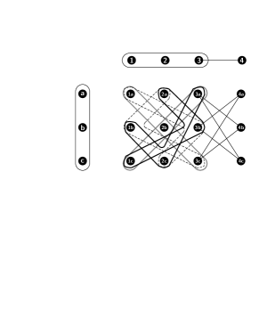
(a) Shown are the non-Cartesian edges of the normal product $H_{1}\mathop{\vbox{\halign{#\cr\kern 3.0pt\cr$\hfil{\scriptscriptstyle\smile}\hfil$\crcr\kern 1.0pt\nointerlineskip\cr$\displaystyle{\boxtimes}$\crcr}}}\,H_{2}$.

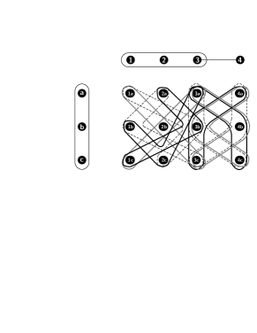
(b) Shown are the non-Cartesian edges of the strong product $H_{1}\mathop{\vbox{\halign{#\cr\kern 3.0pt\cr$\hfil{\scriptscriptstyle\frown}\hfil$\crcr\kern 1.0pt\nointerlineskip\cr$\displaystyle{\boxtimes}$\crcr}}}\,H_{2}$.

(d) Shown is the 2-section $[H_{1}]_{2}\boxtimes[H_{2}]_{2}=[H_{1}\mathop{\vbox{\halign{#\cr\kern 3.0pt\cr$\hfil{\scriptscriptstyle\smile}\hfil$\crcr\kern 1.0pt\nointerlineskip\cr$\displaystyle{\boxtimes}$\crcr}}}\,H_{2}]_{2}=[H_{1}\mathop{\vbox{\halign{#\cr\kern 3.0pt\cr$\hfil{\scriptscriptstyle\frown}\hfil$\crcr\kern 1.0pt\nointerlineskip\cr$\displaystyle{\boxtimes}$\crcr}}}\,H_{2}]_{2}$

Figure 1: Depicted are the Cartesian and non-Cartesian edges of the different products under investigation. The non-Cartesian edges are drawn in different line-styles, to improve visualization. The hypergraph factors $H_{1}$ and $H_{2}$ are not thin, and thus neither $H_{1}\mathop{\vbox{\halign{#\cr\kern 3.0pt\cr$\hfil{\scriptscriptstyle\smile}\hfil$\crcr\kern 1.0pt\nointerlineskip\cr$\displaystyle{\boxtimes}$\crcr}}}\,H_{2}$ nor $H_{1}\mathop{\vbox{\halign{#\cr\kern 3.0pt\cr$\hfil{\scriptscriptstyle\frown}\hfil$\crcr\kern 1.0pt\nointerlineskip\cr$\displaystyle{\boxtimes}$\crcr}}}\,H_{2}$ is.

            
            

(c) Shown is the Cartesian product $H_{1}\Box H_{2}$.

Remark 2.

For the normal product $H=H_{1}\mathop{\vbox{\halign{#\cr\kern 3.0pt\cr$\hfil{\scriptscriptstyle\smile}\hfil$\crcr\kern 1.0pt\nointerlineskip\cr$\displaystyle{\boxtimes}$\crcr}}}\,H_{2}$ and an edge $e\in E(H)$ holds, if $p_{i}(e)\subseteq e_{i}\in E(H_{i})$ then $|e|\leq|e_{i}|$. In particular, $p_{i}(e)\subseteq e_{i}\in E(H_{i})$ and $|e|=|e_{i}|$ implies that $p_{i}(e)=e_{i}\in E(H_{i})$, $i\in\{1,2\}$.

For the strong product $H=H_{1}\mathop{\vbox{\halign{#\cr\kern 3.0pt\cr$\hfil{\scriptscriptstyle\frown}\hfil$\crcr\kern 1.0pt\nointerlineskip\cr$\displaystyle{\boxtimes}$\crcr}}}\,H_{2}$ and an edge $e\in E(H)$ holds, if $p_{i}(e)=e_{i}\in E(H_{i})$ then $|e|\geq|e_{i}|$. In particular, $p_{i}(e)=e_{i}\in E(H_{i})$ and $|e|=|e_{i}|$ implies that $p_{i}(x)\neq p_{i}(y)$ for all $x,y\in e$ with $x\neq y$, $i\in\{1,2\}$.

These three hypergraph products are associative and commutative, thus the product of finitely many factors is well defined. The one-vertex hypergraph $K_{1}$ without edges serves as unit element for the Cartesian, normal and strong product, that is, it holds the trivial product representation $K_{1}\circledast H\cong H$, for all $H$ and $\circledast\in\{\Box,\mathop{\vbox{\halign{#\cr\kern 3.0pt\cr$\hfil{\scriptscriptstyle\smile}\hfil$\crcr\kern 1.0pt\nointerlineskip\cr$\displaystyle{\boxtimes}$\crcr}}}\,,\mathop{\vbox{\halign{#\cr\kern 3.0pt\cr$\hfil{\scriptscriptstyle\frown}\hfil$\crcr\kern 1.0pt\nointerlineskip\cr$\displaystyle{\boxtimes}$\crcr}}}\,\}$. A hypergraph is prime w.r.t. $\circledast\in\{\Box,\mathop{\vbox{\halign{#\cr\kern 3.0pt\cr$\hfil{\scriptscriptstyle\smile}\hfil$\crcr\kern 1.0pt\nointerlineskip\cr$\displaystyle{\boxtimes}$\crcr}}}\,,\mathop{\vbox{\halign{#\cr\kern 3.0pt\cr$\hfil{\scriptscriptstyle\frown}\hfil$\crcr\kern 1.0pt\nointerlineskip\cr$\displaystyle{\boxtimes}$\crcr}}}\,\}$ if it has only a trivial product representation. The Cartesian, normal and strong product of connected hypergraphs is always connected [9]. Moreover, it is known that every connected hypergraph $H=(V,E)$ has a unique prime factor decomposition w.r.t. (weak) Cartesian product [11, 14]. Furthermore, the number $k$ of Cartesian prime factors of $H=(V,E)$ is bounded by $\log_{2}(|V|)$, since every Cartesian product of $k$ non-trivial hypergraphs has at least $2^{k}$ vertices.

Having associativity we can conclude, that a vertex $x$ in these three products $\circledast_{i\in I}H_{i}$, $\circledast\in\{\Box,\mathop{\vbox{\halign{#\cr\kern 3.0pt\cr$\hfil{\scriptscriptstyle\smile}\hfil$\crcr\kern 1.0pt\nointerlineskip\cr$\displaystyle{\boxtimes}$\crcr}}}\,,\mathop{\vbox{\halign{#\cr\kern 3.0pt\cr$\hfil{\scriptscriptstyle\frown}\hfil$\crcr\kern 1.0pt\nointerlineskip\cr$\displaystyle{\boxtimes}$\crcr}}}\,\}$ is properly “coordinatized” by the vector $(x_{1},\dots,x_{|I|})$ whose entries are the vertices $x_{i}$ of its factors $H_{i}$. Two adjacent vertices in the Cartesian product, respectively vertices of a Cartesian edge in the normal and the strong product, therefore differ in exactly one coordinate. Moreover, the coordinatization of a product is equivalent to a (partial) edge coloring of $H$ in which edges $e$ share the same color $c(e)=k$ if all $x,y\in e$ differ only in the value of a single coordinate $k$, i.e., if $x_{i}=y_{i}$, $i\neq k$ and $x_{k}\neq y_{k}$. This colors the Cartesian edges of $H$ (with respect to the given product representation). It is easy to see, that for each color $k$ the partial hypergraph $(V^{\prime},E^{\prime})$ with $E^{\prime}=\{e\in E(H)|c(e)=k\}$ as the set of edges with color $k$ and $V^{\prime}=\cup_{e\in E^{\prime}}e$ spans $H=(V,E)$, that is, $V^{\prime}=V$.

For a given vertex $w\in V(H)$, $H=\circledast_{i\in I}H_{i}$ the $H_{j}$-layer (through $w$) is the induced partial hypergraph of $H$

$$H_{j}^{w}=\left\langle\{v\in V(H)\mid p_{k}(v)=p_{k}(w)\text{ for }k\neq j\}\right\rangle.$$

For $\circledast\in\{\Box,\mathop{\vbox{\halign{#\cr\kern 3.0pt\cr$\hfil{\scriptscriptstyle\smile}\hfil$\crcr\kern 1.0pt\nointerlineskip\cr$\displaystyle{\boxtimes}$\crcr}}}\,,\mathop{\vbox{\halign{#\cr\kern 3.0pt\cr$\hfil{\scriptscriptstyle\frown}\hfil$\crcr\kern 1.0pt\nointerlineskip\cr$\displaystyle{\boxtimes}$\crcr}}}\,\}$, we have $H_{j}^{w}\cong H_{j}$ for all $j\in I,\,w\in V(H)$ [9].

Furthermore, for sake of convenience, we introduce the following notations. Let $H_{1}$ and $H_{2}$ be hypergraphs and $\circledast\in\{\Box,\mathop{\vbox{\halign{#\cr\kern 3.0pt\cr$\hfil{\scriptscriptstyle\smile}\hfil$\crcr\kern 1.0pt\nointerlineskip\cr$\displaystyle{\boxtimes}$\crcr}}}\,,\mathop{\vbox{\halign{#\cr\kern 3.0pt\cr$\hfil{\scriptscriptstyle\frown}\hfil$\crcr\kern 1.0pt\nointerlineskip\cr$\displaystyle{\boxtimes}$\crcr}}}\,\}$. For $H_{1}\circledast H_{2}$ let $e_{i}\in E(H_{i}),i=1,2$ and define

$$e_{1}\circledast e_{2}:=(e_{1},\{e_{1}\})\circledast(e_{2},\{e_{2}\}).$$

Note, for $\circledast\in\{\Box,\mathop{\vbox{\halign{#\cr\kern 3.0pt\cr$\hfil{\scriptscriptstyle\smile}\hfil$\crcr\kern 1.0pt\nointerlineskip\cr$\displaystyle{\boxtimes}$\crcr}}}\,,\mathop{\vbox{\halign{#\cr\kern 3.0pt\cr$\hfil{\scriptscriptstyle\frown}\hfil$\crcr\kern 1.0pt\nointerlineskip\cr$\displaystyle{\boxtimes}$\crcr}}}\,\}$ holds $E(e_{1}\circledast e_{2})\subseteq E(H_{1}\circledast H_{2})$. Moreover, for an arbitrary subset $E^{\prime}\subseteq E(H_{1})$ and $x\in V(H_{2})$ we denote by $E^{\prime}\times\{x\}:=\{e\times\{x\}\mid e\in E^{\prime}\}$. For later reference we remark, since $K_{1}$ is the unit element for $\circledast$ we can rewrite $E^{\prime}\times\{x\}=E((V^{\prime},E^{\prime})\circledast(x,\emptyset))$ where $V^{\prime}=\cup_{e\in E^{\prime}}e$.

We now give several useful results, that will be needed later on.

Lemma 2.1 ([9]).

The $2$-section of the product $H^{\prime}\circledast H^{\prime\prime}$, $\circledast\in\{\Box,\mathop{\vbox{\halign{#\cr\kern 3.0pt\cr$\hfil{\scriptscriptstyle\smile}\hfil$\crcr\kern 1.0pt\nointerlineskip\cr$\displaystyle{\boxtimes}$\crcr}}}\,,\mathop{\vbox{\halign{#\cr\kern 3.0pt\cr$\hfil{\scriptscriptstyle\frown}\hfil$\crcr\kern 1.0pt\nointerlineskip\cr$\displaystyle{\boxtimes}$\crcr}}}\,\}$ is the respective graph product of the $2$-section of $H^{\prime}$ and $H^{\prime\prime}$, more formally:

$$[H^{\prime}\circledast H^{\prime\prime}]_{2}=[H^{\prime}]_{2}\circledast[H^{\prime\prime}]_{2}.$$

Lemma 2.2 ([9]).

The product $H^{\prime}\circledast H^{\prime\prime}$, $\circledast\in\{\Box,\mathop{\vbox{\halign{#\cr\kern 3.0pt\cr$\hfil{\scriptscriptstyle\smile}\hfil$\crcr\kern 1.0pt\nointerlineskip\cr$\displaystyle{\boxtimes}$\crcr}}}\,,\mathop{\vbox{\halign{#\cr\kern 3.0pt\cr$\hfil{\scriptscriptstyle\frown}\hfil$\crcr\kern 1.0pt\nointerlineskip\cr$\displaystyle{\boxtimes}$\crcr}}}\,\}$ of simple hypergraphs $H^{\prime}$ and $H^{\prime\prime}$ is simple.

Lemma 2.3 (Distance Formula [9]).

Let $H=(V,E)$ be a hypergraph and $x,y\in V$. Then the distances between $x$ and $y$ in $H$ and in $[H]_{2}$ are the same.

As for the strong graph product $G=G^{\prime}\boxtimes G^{\prime\prime}$ holds that $G$ is thin if and only if $G^{\prime}$ and $G^{\prime\prime}$ are thin [6], we obtain together with the latter lemma the following results.

Corollary 2.4.

Let $H=H^{\prime}\boxtimes H^{\prime\prime}$, $\boxtimes\in\{\mathop{\vbox{\halign{#\cr\kern 3.0pt\cr$\hfil{\scriptscriptstyle\frown}\hfil$\crcr\kern 1.0pt\nointerlineskip\cr$\displaystyle{\boxtimes}$\crcr}}}\,,\mathop{\vbox{\halign{#\cr\kern 3.0pt\cr$\hfil{\scriptscriptstyle\smile}\hfil$\crcr\kern 1.0pt\nointerlineskip\cr$\displaystyle{\boxtimes}$\crcr}}}\,\}$. Then it holds $N^{H}[x]=N^{[H]_{2}}[x]$. Moreover, $H$ is thin if and only if $[H]_{2}$ is thin if and only if $H^{\prime}$ and $H^{\prime\prime}$ are thin.

For later reference we state the next lemma.

Lemma 2.5.

Let $H_{1},H_{2}$ be two hypergraphs. For the number $|\mathop{\vbox{\halign{#\cr\kern 3.0pt\cr$\hfil{\scriptscriptstyle\smile}\hfil$\crcr\kern 1.0pt\nointerlineskip\cr$\displaystyle{\times}$\crcr}}}\,|\,$ of non-Cartesian edges in $H=H_{1}\mathop{\vbox{\halign{#\cr\kern 3.0pt\cr$\hfil{\scriptscriptstyle\smile}\hfil$\crcr\kern 1.0pt\nointerlineskip\cr$\displaystyle{\boxtimes}$\crcr}}}\,H_{2}$ holds

$$|\mathop{\vbox{\halign{#\cr\kern 3.0pt\cr$\hfil{\scriptscriptstyle\smile}\hfil$\crcr\kern 1.0pt\nointerlineskip\cr$\displaystyle{\times}$\crcr}}}\,|\,:=|E(H_{1}\mathop{\vbox{\halign{#\cr\kern 3.0pt\cr$\hfil{\scriptscriptstyle\smile}\hfil$\crcr\kern 1.0pt\nointerlineskip\cr$\displaystyle{\boxtimes}$\crcr}}}\,H_{2})\setminus E(H_{1}\Box H_{2})|=\sum_{e_{1}\in E_{1},e_{2}\in E_{2}}\frac{(\max\{|e_{1}|,|e_{2}|\})!}{\big{|}|e_{1}|-|e_{2}|\big{|}!}.$$

For the number $|\mathop{\vbox{\halign{#\cr\kern 3.0pt\cr$\hfil{\scriptscriptstyle\frown}\hfil$\crcr\kern 1.0pt\nointerlineskip\cr$\displaystyle{\times}$\crcr}}}\,|\,$ of non-Cartesian edges in $H=H_{1}\mathop{\vbox{\halign{#\cr\kern 3.0pt\cr$\hfil{\scriptscriptstyle\frown}\hfil$\crcr\kern 1.0pt\nointerlineskip\cr$\displaystyle{\boxtimes}$\crcr}}}\,H_{2}$ holds

$$|\mathop{\vbox{\halign{#\cr\kern 3.0pt\cr$\hfil{\scriptscriptstyle\frown}\hfil$\crcr\kern 1.0pt\nointerlineskip\cr$\displaystyle{\times}$\crcr}}}\,|\,:=|E(H_{1}\mathop{\vbox{\halign{#\cr\kern 3.0pt\cr$\hfil{\scriptscriptstyle\frown}\hfil$\crcr\kern 1.0pt\nointerlineskip\cr$\displaystyle{\boxtimes}$\crcr}}}\,H_{2})\setminus E(H_{1}\Box H_{2})|=\sum_{e_{1}\in E_{1},e_{2}\in E_{2}}(\min\{|e_{1}|,|e_{2}|\})!S_{\max\{|e_{1}|,|e_{2}|\},\min\{|e_{1}|,|e_{2}|\}},$$

where $S_{n,k}$ denotes the the Stirling number of the second kind $S_{n,k}=\frac{1}{k!}\sum_{j=0}^{k}(-1)^{k-j}\binom{k}{j}j^{n}.$

Proof.

To prove validity of the formula for $|\mathop{\vbox{\halign{#\cr\kern 3.0pt\cr$\hfil{\scriptscriptstyle\smile}\hfil$\crcr\kern 1.0pt\nointerlineskip\cr$\displaystyle{\times}$\crcr}}}\,|\,$, we show that $e$ is a non-Cartesian edge in $H_{1}\mathop{\vbox{\halign{#\cr\kern 3.0pt\cr$\hfil{\scriptscriptstyle\smile}\hfil$\crcr\kern 1.0pt\nointerlineskip\cr$\displaystyle{\boxtimes}$\crcr}}}\,H_{2}$ if and only if there are edges $e_{1}\in E(H_{1})$ and $e_{2}\in E(H_{2})$ such that $p_{1}(x)\mapsto p_{2}(x)$ for all $x\in e$ defines an injective mapping $e_{1}\to e_{2}$ whenever $|e_{1}|\leq|e_{2}|$ and else that $p_{2}(x)\mapsto p_{1}(x)$ for all $x\in e$ defines an injective mapping $e_{2}\to e_{1}$.

Let $e$ be a non-Cartesian edge in $H_{1}\mathop{\vbox{\halign{#\cr\kern 3.0pt\cr$\hfil{\scriptscriptstyle\smile}\hfil$\crcr\kern 1.0pt\nointerlineskip\cr$\displaystyle{\boxtimes}$\crcr}}}\,H_{2}$. Clearly, by definition of the normal product, there are edges $e_{1}\in E(H_{1})$ and $e_{2}\in E(H_{2})$ with $e\in E(e_{1}\mathop{\vbox{\halign{#\cr\kern 3.0pt\cr$\hfil{\scriptscriptstyle\smile}\hfil$\crcr\kern 1.0pt\nointerlineskip\cr$\displaystyle{\boxtimes}$\crcr}}}\,e_{2})$. Assume w.l.o.g. $|e_{1}|\leq|e_{2}|$, otherwise interchange the role of $e_{1}$ and $e_{2}$. By definition of the normal product it holds $|p_{1}(e)|=|p_{2}(e)|=|e|=|e_{1}|\leq|e_{2}|$. Thus, we have $p_{1}(e)=e_{1}\in E(H_{1})$. Therefore, we can conclude that all vertices of $e$ differ in each coordinate, and thus, $p_{1}(x)\neq p_{1}(x^{\prime})$ implies $p_{2}(x)\neq p_{2}(x^{\prime})$ for all distinct vertices $x,x^{\prime}\in e$. Since $p_{2}(e)\subseteq e_{2}$, it follows that $p_{1}(x)\mapsto p_{2}(x)$, $x\in e$ indeed defines an injective mapping $e_{1}\to e_{2}$. Conversely, if there are edges $e_{1}\in E(H_{1})$ and $e_{2}\in E(H_{2})$ such that w.l.o.g. $p_{1}(x)\mapsto p_{2}(x)$, $x\in e$ defines an injective mapping $e_{1}\to e_{2}$, we can conclude that $p_{1}(e)=e_{1}$ and $p_{2}(e)\subseteq e_{2}$. Since $p_{1}(x)\mapsto p_{2}(x)$, $x\in e$ is a mapping, we have $|e|=|e_{1}|$ and by injectivity, it follows $|e_{1}|=|p_{1}(e)|=|p_{2}(e)|\leq|e_{2}|$. Hence, $e$ satisfies the condition $(ii)$ in the definition of the edges in the normal product and thus, $e\in E(H_{1}\mathop{\vbox{\halign{#\cr\kern 3.0pt\cr$\hfil{\scriptscriptstyle\smile}\hfil$\crcr\kern 1.0pt\nointerlineskip\cr$\displaystyle{\boxtimes}$\crcr}}}\,H_{2})$. Finally, it is well-known, that for any two sets $N$, $M$ with $|N|\leq|M|$ there are $\frac{|M|!}{(|M|-|N|)!}$ injective mappings from $N$ to $M$. Applying this result to every pair of edges $e_{1}\in E(H_{1})$ and $e_{2}\in E(H_{2})$ the assertion for $|\mathop{\vbox{\halign{#\cr\kern 3.0pt\cr$\hfil{\scriptscriptstyle\smile}\hfil$\crcr\kern 1.0pt\nointerlineskip\cr$\displaystyle{\times}$\crcr}}}\,|\,$ follows.

To prove validity of the formula for $|\mathop{\vbox{\halign{#\cr\kern 3.0pt\cr$\hfil{\scriptscriptstyle\frown}\hfil$\crcr\kern 1.0pt\nointerlineskip\cr$\displaystyle{\times}$\crcr}}}\,|\,$, we show that $e$ is a non-Cartesian edge in $H_{1}\mathop{\vbox{\halign{#\cr\kern 3.0pt\cr$\hfil{\scriptscriptstyle\frown}\hfil$\crcr\kern 1.0pt\nointerlineskip\cr$\displaystyle{\boxtimes}$\crcr}}}\,H_{2}$ if and only if there are edges $e_{1}\in E(H_{1})$ and $e_{2}\in E(H_{2})$ such that $p_{1}(x)\mapsto p_{2}(x)$ for all $x\in e$ defines a surjective mapping $e_{1}\to e_{2}$ whenever $|e_{1}|\geq|e_{2}|$ and else that $p_{2}(x)\mapsto p_{1}(x)$ for all $x\in e$ defines a surjective mapping $e_{2}\to e_{1}$.

Let $e$ be a non-Cartesian edge in $H_{1}\mathop{\vbox{\halign{#\cr\kern 3.0pt\cr$\hfil{\scriptscriptstyle\frown}\hfil$\crcr\kern 1.0pt\nointerlineskip\cr$\displaystyle{\boxtimes}$\crcr}}}\,H_{2}$. Clearly, by definition of the strong product, there are edges $e_{1}\in E(H_{1})$ and $e_{2}\in E(H_{2})$ with $e\in E(e_{1}\mathop{\vbox{\halign{#\cr\kern 3.0pt\cr$\hfil{\scriptscriptstyle\frown}\hfil$\crcr\kern 1.0pt\nointerlineskip\cr$\displaystyle{\boxtimes}$\crcr}}}\,e_{2})$. Assume w.l.o.g. $|e_{1}|\geq|e_{2}|$, otherwise interchange the role of $e_{1}$ and $e_{2}$. By definition of the strong product it holds that $|e|=|e_{1}|$ and $p_{1}(e)=e_{1}$ which implies that $p_{1}(x)\neq p_{1}(x^{\prime})$ for all distinct vertices $x,x^{\prime}\in e$. Thus, $p_{1}(x)\mapsto p_{2}(x)$ indeed defines a mapping $e_{1}\to e_{2}$. Since $p_{2}(e)=e_{2}$, this mapping is surjective. Conversely, if there are edges $e_{1}\in E(H_{1})$ and $e_{2}\in E(H_{2})$ such that w.l.o.g. $p_{1}(x)\mapsto p_{2}(x)$, $x\in e$ defines a surjective mapping $e_{1}\to e_{2}$ we can conclude that $p_{1}(e)=e_{1}$ and $p_{2}(e)=e_{2}$ and thus, in particular that $|p_{1}(e)|=|e_{1}|$. Moreover, it follows that $|e|=|p_{1}(e)|$, since $p_{1}(x)\mapsto p_{2}(x)$ defines a mapping and moreover, $|p_{2}(e)|\leq|p_{1}(e)|=|e_{1}|$, since this mapping is surjective. Hence, $e$ satisfies the condition $(ii)$ in the definition of the edges in the strong product and thus, $e\in E(H_{1}\mathop{\vbox{\halign{#\cr\kern 3.0pt\cr$\hfil{\scriptscriptstyle\frown}\hfil$\crcr\kern 1.0pt\nointerlineskip\cr$\displaystyle{\boxtimes}$\crcr}}}\,H_{2})$. Finally, it is well-known, that for any two sets $N$, $M$ with $|N|\geq|M|$ there are $|M|!S_{|N|,|M|}$ surjective mappings from $N$ to $M$. Applying this result to every pair of edges $e_{1}\in E(H_{1})$ and $e_{2}\in E(H_{2})$ the assertion for $|\mathop{\vbox{\halign{#\cr\kern 3.0pt\cr$\hfil{\scriptscriptstyle\frown}\hfil$\crcr\kern 1.0pt\nointerlineskip\cr$\displaystyle{\times}$\crcr}}}\,|\,$ follows. ∎

Remark 3.

In the sequel of this paper, we will use the symbol $\boxtimes$ for both products, that is, $\boxtimes\in\{\mathop{\vbox{\halign{#\cr\kern 3.0pt\cr$\hfil{\scriptscriptstyle\smile}\hfil$\crcr\kern 1.0pt\nointerlineskip\cr$\displaystyle{\boxtimes}$\crcr}}}\,,\mathop{\vbox{\halign{#\cr\kern 3.0pt\cr$\hfil{\scriptscriptstyle\frown}\hfil$\crcr\kern 1.0pt\nointerlineskip\cr$\displaystyle{\boxtimes}$\crcr}}}\,\}$, unless there is a risk of confusion.

3 The Cartesian Skeleton and PFD Uniqueness Results

3.1 The Cartesian Skeleton

For graphs $G$, the key idea of finding the PFD with respect to the strong product is to find the PFD of a subgraph $\mathbb{S}\,(G)$ of $G$, the so-called Cartesian skeleton, with respect to the Cartesian product and construct the prime factors of $G$ using the information of the PFD of $\mathbb{S}\,(G)$. This concept was first introduced for graphs by Feigenbaum and Schäffer in [4] and later on improved by Hammack and Imrich, see [5]. Following the approach of Hammack and Imrich, one removes edges in $G$ that fulfill so-called dispensability conditions, resulting in a subgraph $\mathbb{S}\,(G)$ that is the desired Cartesian skeleton. The underlying concept of dispensability as defined for graphs in [5] can be generalized in a natural way for hypergraphs.

Definition 3.6 (Dispensability).

An edge $e\in E(H)$ is dispensable in $H$ if there exists a vertex $z\in V(H)$ and distinct vertices $x,y\in e$ for which both of the following statements hold:

1. $N[x]\cap N[y]\subset N[x]\cap N[z]\text{ or }N[x]\subset N[z]\subset N[y]$

2. $N[x]\cap N[y]\subset N[y]\cap N[z]\text{ or }N[y]\subset N[z]\subset N[x]$.

Note, the latter definition coincides with the one given in [5], if $H$ is a simple graph. Now, we are able to define the Cartesian skeleton for hypergraphs.

Definition 3.7 (Cartesian Skeleton).

Let $D(H)\subseteq E(H)$ be the set of dispensable edges in a given hypergraph $H$. The Cartesian skeleton of a hypergraph $H$ is the partial hypergraph $\mathbb{S}\,[H]\subseteq H$ where all dispensable edges $D(H)$ are removed from $H$, that is $V(\mathbb{S}\,[H])=V(H)$ and $E(\mathbb{S}\,[H])=E(H)\setminus D(H)$.

In the next theorem, we shortly summarize the results established by Hammack and Imrich [5] concerning the Cartesian skeleton of graphs and show in the sequel, that these results can easily be transferred to hypergraphs by usage of its corresponding 2-sections.

Theorem 3.8 ([5]).

Let $G=G_{1}\boxtimes G_{2}$ be a strong product graph.

1. If $G$ is thin then every non-dispensable edge $e\in E(G)$ is Cartesian w.r.t. any factorization $G^{\prime}_{1}\boxtimes G_{2}^{\prime}$ of $G$.

2. If $G$ is connected, then $\mathbb{S}\,(G)$ is connected.

3. If $G_{1}$ and $G_{2}$ are thin graphs then $\mathbb{S}\,(G_{1}\boxtimes G_{2})=\mathbb{S}\,(G_{1})\Box\mathbb{S}\,(G_{2}).$

4. Any isomorphism $\varphi:G\rightarrow H$, as a map $V(G)\rightarrow V(H)$, is also an isomorphism $\varphi:\mathbb{S}\,(G)\rightarrow\mathbb{S}\,(H)$.

Since neighborhoods of vertices in a hypergraph and its 2-section are identical by Corollary 2.4 and dispensability is defined only in terms of neighborhoods, we easily obtain the following lemma and corollary.

Lemma 3.9.

Let $H$ be a hypergraph. The edge $e\in E(H)$ is dispensable in $H$ if and only if there is an edge $e^{\prime}\in E([H]_{2})$ with $e^{\prime}\subseteq e$ and $e^{\prime}$ is dispensable in $[H]_{2}$.

Corollary 3.10.

For all hypergraphs $H$ holds: $[\mathbb{S}\,(H)]_{2}=\mathbb{S}\,([H]_{2})$.

From the Distance Formula and Theorem 3.8 we obtain immediately:

Corollary 3.11.

For all hypergraphs $H$ holds: If $H$ is connected then $\mathbb{S}\,(H)$ is connected.

Lemma 3.12.

Let $H$ be a hypergraph and $H_{1}\boxtimes H_{2}$ be an arbitrary factorization of $H$. Then it holds that the edge $e$ is Cartesian in $H$ w.r.t. $H_{1}\boxtimes H_{2}$ if and only if $e^{\prime}$ is Cartesian in $[H_{1}]_{2}\boxtimes[H_{2}]_{2}=[H]_{2}$ for all $e^{\prime}\subseteq e$ with $e^{\prime}\in E([H]_{2})$.

Proof.

Let $e\in E(H)$ be Cartesian w.r.t. to its factorization $H_{1}\boxtimes H_{2}$. Then, there is an $i\in\{1,2\}$ with $|p_{i}(e)|=1$. Moreover, for all $e^{\prime}\subseteq e$ it holds, $0<|p_{i}(e^{\prime})|\leq|p_{i}(e)|=1$ and hence, $|p_{i}(e^{\prime})|=1$. Therefore, each edge $e^{\prime}\in E([H]_{2})$ with $e^{\prime}\subseteq e$ is Cartesian in $[H]_{2}=[H_{1}]_{2}\boxtimes[H_{2}]_{2}$.

By contraposition, assume $e\in E(H)$ is non-Cartesian w.r.t. $H_{1}\boxtimes H_{2}$. Hence, by definition of the products $\mathop{\vbox{\halign{#\cr\kern 3.0pt\cr$\hfil{\scriptscriptstyle\smile}\hfil$\crcr\kern 1.0pt\nointerlineskip\cr$\displaystyle{\boxtimes}$\crcr}}}\,$ and $\mathop{\vbox{\halign{#\cr\kern 3.0pt\cr$\hfil{\scriptscriptstyle\frown}\hfil$\crcr\kern 1.0pt\nointerlineskip\cr$\displaystyle{\boxtimes}$\crcr}}}\,$ we have $|p_{i}(e)|>1$, $i=1,2$. Therefore, there are vertices $x,y\in e$ with $p_{1}(x)\neq p_{1}(y)$. If $p_{2}(x)\neq p_{2}(y)$ it follows that $e^{\prime}=\{x,y\}$ is non-Cartesian in $[H]_{2}=[H_{1}]_{2}\boxtimes[H_{2}]_{2}$. If $p_{2}(x)=p_{2}(y)$ then there is a vertex $z\in e$ with $p_{2}(x)\neq p_{2}(z)$. If $p_{1}(z)\neq p_{1}(x)$ then the edge $e^{\prime}=\{x,z\}$ is non-Cartesian in $[H]_{2}=[H_{1}]_{2}\boxtimes[H_{2}]_{2}$ and if $p_{1}(z)=p_{1}(x)\neq p_{1}(y)$ then the edge $e^{\prime}=\{y,z\}$ is non-Cartesian in $[H]_{2}=[H_{1}]_{2}\boxtimes[H_{2}]_{2}$. ∎

Lemma 3.13.

Let $H$ be a thin hypergraph. If $e\in E(H)$ is non-dispensable in $H$ then the edge $e$ is Cartesian w.r.t. any factorization $H_{1}\boxtimes H_{2}$ of $H$.

Proof.

Let $e\in E(H)$ be non-dispensable in $H$. Lemma 3.9 implies that for all $e^{\prime}\in E([H]_{2})$ with $e^{\prime}\subseteq e$ holds $e^{\prime}$ is non-dispensable in $[H]_{2}$. Furthermore, by Corollary 2.4 it holds that $[H]_{2}$ is thin. Thus, Theorem 3.8 implies that $e^{\prime}$ is Cartesian in $[H]_{2}$ for all $e^{\prime}\subseteq e$, which is by Lemma 3.12 if and only if $e$ is Cartesian in $H$. ∎

Proposition 3.14.

If $H_{1}$ and $H_{2}$ are thin hypergraphs, then $\mathbb{S}\,(H_{1}\boxtimes H_{2})=\mathbb{S}\,(H_{1})\Box\mathbb{S}\,(H_{2})$.

Proof.

Let $H=H_{1}\boxtimes H_{2}$. Lemma 3.13 implies that every non-Cartesian edge is dispensable. Hence we need to show, that a Cartesian edge $e\in E(H)$ is dispensable if and only if $p_{i}(e)$ is dispensable whenever $p_{i}(e)\in E(H_{i})$, $i=1,2$. Note, exactly for one $i\in\{1,2\}$ holds $p_{i}(e)\in E(H_{i})$ and $p_{j}(e)\in V(H_{j})$, $j\neq i$. W.l.o.g. assume $p_{1}(e)=e_{1}\in E(H_{1})$ and $p_{2}(e)=v_{2}\in V(H_{2})$.

Assume that the edge $e$ is dispensable in $H$. Then by Lemma 3.9 there exists a dispensable edge $e^{\prime}\in E([H]_{2})$ with $e^{\prime}\subseteq e$. Corollary 2.4 implies that $[H]_{2}$ is thin and by Theorem 3.8 it holds that $\mathbb{S}\,([H]_{2})=\mathbb{S}\,([H_{1}]_{2})\Box\mathbb{S}\,([H_{2}]_{2})$ and hence, we infer $p_{1}(e^{\prime})$ must be dispensable in $[H_{1}]_{2}$. Since $p_{1}(e^{\prime})\subseteq e_{1}$ and by Lemma 3.9, we conclude that $e_{1}$ is dispensable in $H_{1}$.

Now suppose $e_{1}$ is dispensable in $H_{1}$. Again by Lemma 3.9, there exists a dispensable edge $e_{1}^{\prime}\in E([H_{1}]_{2})$ such that $e_{1}^{\prime}\subseteq e_{1}$. Again, by Corollary 2.4 it holds that $[H]_{2}$ is thin and Theorem 3.8 implies $\mathbb{S}\,([H]_{2})=\mathbb{S}\,([H_{1}]_{2})\Box\mathbb{S}\,([H_{2}]_{2})$. Therefore, $e^{\prime}=e_{1}^{\prime}\times\{v_{2}\}$ is dispensable in $[H]_{2}$. By Lemma 3.9 and since $e^{\prime}\subseteq e$, we have $e$ is dispensable in $H$. ∎

As in [5] the Cartesian skeleton $\mathbb{S}\,(H)$ is defined entirely in terms of the adjacency structure of $H$, and thus, we obtain the following immediate consequence of the definition.

Proposition 3.15.

Any isomorphism $\varphi:H\rightarrow G$, as a map $V(H)\rightarrow V(G)$, is also an isomorphism $\varphi:\mathbb{S}\,[H]\rightarrow\mathbb{S}\,[G].$

3.2 Prime Factorization Theorem

In the following, let $\boxtimes\in\{\mathop{\vbox{\halign{#\cr\kern 3.0pt\cr$\hfil{\scriptscriptstyle\smile}\hfil$\crcr\kern 1.0pt\nointerlineskip\cr$\displaystyle{\boxtimes}$\crcr}}}\,,\mathop{\vbox{\halign{#\cr\kern 3.0pt\cr$\hfil{\scriptscriptstyle\frown}\hfil$\crcr\kern 1.0pt\nointerlineskip\cr$\displaystyle{\boxtimes}$\crcr}}}\,\}$. Let $A\boxtimes B$ and $C\boxtimes D$ be two non-trivial decompositions of a simple connected thin hypergraph $H$. We will show that then $H$ has a finer factorization of the form $AC\boxtimes AD\boxtimes BC\boxtimes BD$ and $A=AC\boxtimes AD$, $B=BC\boxtimes BD$, C=$AC\boxtimes BC$ and $D=AD\boxtimes BD$, see Prop. 3.22. Similar as for graphs [12, page 171-174], this can be used to show that every simple thin connected hypergraph has a unique prime factorization with respect to the normal and strong (hypergraph) product. We don’t want to conceal the fact, that in the sequel of this section, we make frequent use of the same arguments as for graph products in [12] and [6].

By Proposition 3.14, it holds $\mathbb{S}\,(H)=\mathbb{S}\,(A)\Box\mathbb{S}\,(B)=\mathbb{S}\,(C)\Box\mathbb{S}\,(D)$. Let $\mathbb{S}\,(H)=\Box_{i\in I}H_{i}$ be the unique PFD of the Cartesian skeleton of $H$. Hence, the factors $\mathbb{S}\,(A)$, $\mathbb{S}\,(B)$, $\mathbb{S}\,(C)$ and $\mathbb{S}\,(D)$ are all products of or isomorphic to the Cartesian prime factors of $\mathbb{S}\,(H)$. Let $I_{A}$ be the subset of the index set $I$ with $V(A)=V(\Box_{i\in I_{A}}H_{i})$. Analogously, the index sets $I_{B}$, $I_{C}$ and $I_{D}$ are defined.

In the following, we define the hypergraphs $AC,AD,BC$ and $BD$ and as it will turn out it holds $H\cong AC\boxtimes AD\boxtimes BC\boxtimes BD$. Therefore, it will be convenient to use only four coordinates $x=(x_{AC},x_{AD},x_{BC},x_{BD})$ for every vertex $x\in V(H)$. With this notation, the projections $p_{AC}:V(H)\rightarrow V(AC)$, $p_{AD}:V(H)\rightarrow V(AD)$, $p_{BC}:V(H)\rightarrow V(BC)$, $p_{BD}:V(H)\rightarrow V(BD)$ are well-defined.

Moreover, the vertex set of $AC$ is defined as $V(AC)=V(\Box_{i\in I_{A}\cap I_{C}}H_{i})$. Analogously, the vertex sets of $AD$, $BC$ and $BD$ are defined. It will be shown that $A=AC\boxtimes AD$, $B=BC\boxtimes BD$, C=$AC\boxtimes BC$ and $D=AD\boxtimes BD$. Of course it is possible that not all of the intersections $I_{A}\cap I_{C},I_{A}\cap I_{D},I_{B}\cap I_{C}$ and $I_{B}\cap I_{D}$ are nonempty. Suppose that $I_{B}\cap I_{D}=\emptyset$ then $I_{A}\cap I_{D}\neq\emptyset$, since otherwise $I_{D}=\emptyset$. If in addition $I_{A}\cap I_{C}$ were empty, then $I_{A}=I_{D}$ and thus $I_{B}=I_{C}$, but then there would be nothing to prove. Thus, we can assume that all but possibly $I_{B}\cap I_{D}$ are nonempty and at least three of the four coordinates are nontrivial, that is to say, there are at least two vertices that differ in the first, second and third coordinates, but it is possible that all vertices have the same fourth coordinate.

With the definition of the projections $p_{A},p_{B},p_{C}$ and $p_{D}$ together with the preceding construction of the coordinates $(x_{AC},x_{AD},x_{BC},x_{BD})$ for vertices $x\in V(H)$, we thus have

$$x_{A}=p_{A}(x)=p_{A}(x_{AC},x_{AD},x_{BC},x_{BD})=(x_{AC},x_{AD},-,-)=:(x_{AC},x_{AD})\in V(A),$$

$$x_{B}=p_{B}(x)=p_{B}(x_{AC},x_{AD},x_{BC},x_{BD})=(-,-,x_{BC},x_{BD})=:(x_{BC},x_{BD})\in V(B),$$

$$x_{C}=p_{C}(x)=p_{C}(x_{AC},x_{AD},x_{BC},x_{BD})=(x_{AC},-,x_{BC},-)=:(x_{AC},x_{BC})\in V(C),$$

$$x_{D}=p_{D}(x)=p_{D}(x_{AC},x_{AD},x_{BC},x_{BD})=(-,x_{AD},-,x_{BD})=:(x_{AD},x_{BD})\in V(D).$$

In this way, vertices of $A$, $B$, $C$ and $D$ are coordinatized. Thus, the projections $p^{\prime}_{AC}:V(A)\rightarrow V(AC)$ and $p^{\prime\prime}_{AC}:V(C)\rightarrow V(AC)$ are well-defined. Since for all $x\in V(H)$ holds that

$$p_{AC}(x)=p^{\prime}_{AC}(p_{A}(x))=p^{\prime}_{AC}(x_{A})=p^{\prime\prime}_{AC}(p_{C}(x))=p^{\prime\prime}_{AC}(x_{C})=x_{AC},$$

we will identify $p_{AC}$ with $p^{\prime}_{AC}$, resp., $p^{\prime\prime}_{AC}$, henceforth and simply write $p_{AC}$. Analogously, we identify the respective projections onto $AD$, $BC$ and $BD$ with $p_{AD}$, $p_{BC}$, $p_{BD}$.

We are now in the position to give the complete definition of the hypergraphs $AC$, $AD$, $BC$ and $BD$. The vertex set of $AC$ is

$$V(AC)=V(\Box_{i\in I_{A}\cap I_{C}}H_{i})=\mathop{\hbox{\Large{$\times$}}}_{i\in I_{A}\cap I_{C}}V(H_{i})$$ (1)

The edge set of $AC$ is

$$E(AC)=\{e_{AC}\subseteq V(AC)\mid\exists e_{H}\in E(H)\text{ with }p_{AC}(e_{H})=e_{AC}\text{ s.t. }\nexists e^{\prime}_{H}\in E(H):p_{AC}(e_{H})\subset p_{AC}(e^{\prime}_{H})\}$$ (2)

Analogously, the hypergraphs $AD,BC$ and $BD$ are defined.

Equation (2), that characterizes the edge sets for the (putative) finer factors $AC,AD,BC$ and $BD$ w.r.t. $\boxtimes$, forces edges to be maximal with respect to inclusion. We need this definition, in particular for defining the factors of the normal product, since projections of edges into the factors might be proper subsets of edges different from a single vertex.

Remark 4.

Note, that vertices $x$ are well defined by their entries $x_{AC}$, $x_{AD}$, $x_{BC}$ and $x_{BD}$ of their coordinates, independently from the ordering of $x_{AC}$, $x_{AD}$, $x_{BC}$ and $x_{BD}$, since the coordinates will be clearly marked. Therefore, we henceforth distinguish vertices just by the entries of their coordinates rather than by the ordering.

Lemma 3.16.

Let $H\cong A\boxtimes B\cong C\boxtimes D$ be a thin hypergraph and $AC$ be as defined in Equations (1) and (2). Then it holds:

1. $e_{AC}\subseteq p_{AC}(e_{A})$ implies $e_{AC}=p_{AC}(e_{A})$ and $e_{AC}\subseteq p_{AC}(e_{C})$ implies $e_{AC}=p_{AC}(e_{C})$ for all edges $e_{AC}\in E(AC)$, $e_{A}\in E(A)$ and $e_{C}\in E(C)$.

2. If $p_{AC}(e_{H})\in E(AC)$ then $p_{A}(e_{H})\in E(A)$ and $p_{C}(e_{H})\in E(C)$ for every edge $e_{H}\in E(H)$.

Analogous results hold for the hypergraphs $AD$, $BC$ and $BD$ with respective edges.

Proof.

For the proof of the first statement, let $e_{AC}\in E(AC)$ and assume for contradiction, that there is an edge $e_{A}\in E(A)$ with $e_{AC}\subset p_{AC}(e_{A})$. Thus, there is an edge $e_{H}\in E(H)$ with $e_{H}=e_{A}\times\{x_{B}\},x_{B}\in V(B)$ and therefore, $e_{AC}\subset p_{AC}(e_{H})$, which contradicts the definition of $AC$. Analogously, there is no edge $e_{C}\in E(C)$. such that $e_{AC}\subset p_{AC}(e_{C})$.

For the proof of the second statement, let $e_{H}\in E(H)$ be an arbitrary edge and assume that $p_{AC}(e_{H})\in E(AC)$. Note, if $|p_{AC}(e_{H})|>1$ then there are at least two distinct vertices $x,x^{\prime}\in e_{H}\in E(H)$ with $p_{AC}(x)=x_{AC}\neq p_{AC}(x^{\prime})=x^{\prime}_{AC}$. Hence, $p_{A}(x)\neq p_{A}(x^{\prime})$ and $p_{C}(x)\neq p_{C}(x^{\prime})$. Therefore, $|p_{AC}(e_{H})|>1$ implies that $|p_{A}(e_{H})|>1$ and $|p_{C}(e_{H})|>1$ for each edge $e_{H}\in E(H)$. Thus, whenever $p_{AC}(e_{H})\in E(AC)$ then the projections $p_{A}(e_{H})$ and $p_{C}(e_{H})$ cannot be a single vertex.

If $\boxtimes=\mathop{\vbox{\halign{#\cr\kern 3.0pt\cr$\hfil{\scriptscriptstyle\frown}\hfil$\crcr\kern 1.0pt\nointerlineskip\cr$\displaystyle{\boxtimes}$\crcr}}}\,$ then the condition $p_{A}(e_{H})\in E(A)$ and $p_{C}(e_{H})\in E(C)$ is trivially fulfilled by the definition of $\mathop{\vbox{\halign{#\cr\kern 3.0pt\cr$\hfil{\scriptscriptstyle\frown}\hfil$\crcr\kern 1.0pt\nointerlineskip\cr$\displaystyle{\boxtimes}$\crcr}}}\,$, since $p_{AC}(e_{H})\in E(AC)$ and thus, $|p_{AC}(e_{H})|>1$.

Now, consider the product $\mathop{\vbox{\halign{#\cr\kern 3.0pt\cr$\hfil{\scriptscriptstyle\smile}\hfil$\crcr\kern 1.0pt\nointerlineskip\cr$\displaystyle{\boxtimes}$\crcr}}}\,$. Note, since $e_{H}\in E(e_{A}\mathop{\vbox{\halign{#\cr\kern 3.0pt\cr$\hfil{\scriptscriptstyle\smile}\hfil$\crcr\kern 1.0pt\nointerlineskip\cr$\displaystyle{\boxtimes}$\crcr}}}\,e_{B})$ for some $e_{A}\in E(A)$, $e_{B}\in E(B)$ we can conclude by definition of the normal product that $p_{A}(e_{H})\subseteq e_{A}$ and thus, $p_{AC}(e_{H})=p_{AC}(p_{A}(e_{H}))\subseteq p_{AC}(e_{A})$. By assumption, we have $p_{AC}(e_{H})\in E(AC)$ and therefore, Item $(1)$ of this lemma implies that $p_{AC}(e_{H})=p_{AC}(e_{A})$. Moreover, it holds that $|e_{H}|\geq|p_{AC}(e_{H})|$ and by Remark 2 we have $|e_{A}|\geq|e_{H}|\geq|p_{AC}(e_{H})|$. Since $H\cong A\mathop{\vbox{\halign{#\cr\kern 3.0pt\cr$\hfil{\scriptscriptstyle\smile}\hfil$\crcr\kern 1.0pt\nointerlineskip\cr$\displaystyle{\boxtimes}$\crcr}}}\,B$ there is an edge $e^{\prime}_{H}=e_{A}\times\{x_{B}\}\in E(H)$ which implies that $p_{C}(e^{\prime}_{H})=p_{AC}(e_{A})\times\{x_{BC}\}$. Thus, $|p_{C}(e^{\prime}_{H})|=|p_{AC}(e_{A})|\leq|e_{A}|=|e^{\prime}_{H}|$, since $e^{\prime}_{H}$ is Cartesian w.r.t. $A\mathop{\vbox{\halign{#\cr\kern 3.0pt\cr$\hfil{\scriptscriptstyle\smile}\hfil$\crcr\kern 1.0pt\nointerlineskip\cr$\displaystyle{\boxtimes}$\crcr}}}\,B$. Since $H\cong C\mathop{\vbox{\halign{#\cr\kern 3.0pt\cr$\hfil{\scriptscriptstyle\smile}\hfil$\crcr\kern 1.0pt\nointerlineskip\cr$\displaystyle{\boxtimes}$\crcr}}}\,D$ and by the definition of the normal product it holds $|p_{C}(e_{H}^{\prime})|=|e_{H}^{\prime}|$, and therefore, $|e_{A}|=|p_{AC}(e_{A})|=|p_{AC}(e_{H})|$. Since $|e_{A}|\geq|e_{H}|\geq|p_{AC}(e_{H})|$ it holds $|e_{H}|=|e_{A}|$. Thus, we can conclude by Remark 2 that $p_{A}(e_{H})\in E(A)$. By similar arguments one can show that $p_{C}(e_{H})\in E(C)$. ∎

Lemma 3.17.

Let $H\cong A\boxtimes B\cong C\boxtimes D$ be a thin hypergraph and $AC$ and $BC$ be as defined in Equations (1) and (2). Then for all $e_{AC}\in E(AC)$ and all $x_{BC}\in V(BC)$ there is an edge $e_{C}=e_{AC}\times\{x_{BC}\}\in E(C)$. Analogous results hold for the hypergraphs $AD$, $BC$ and $BD$ with respective edges.

Proof.

Let $e_{AC}\in E(AC)$ be an arbitrary edge. By definition of $AC$, there is an edge $e_{H}\in E(H)$ with $p_{AC}(e_{H})=e_{AC}$. Note, by the same arguments as in the proof of Lemma 3.16 it holds that $|p_{AC}(e_{H})|>1$ implies $|p_{A}(e_{H})|>1$ and $|p_{C}(e_{H})|>1$ for each $e_{H}\in E(H)$.

Since $e_{H}\in E(A\boxtimes B)$, there is an edge $e_{A}\in E(A)$ s.t. $p_{A}(e_{H})\subseteq e_{A}$. Therefore, $e_{AC}=p_{AC}(e_{H})=p_{AC}(p_{A}(e_{H}))\subseteq p_{AC}(e_{A})$ which implies together with Lemma 3.16 (1), that $p_{AC}(e_{A})=e_{AC}$. By Lemma 3.16 (2), we have $p_{A}(e_{H})=e_{A}$. Therefore, there is an edge of the form $e_{A}\times\{x_{B}\}\in E(H)$. W.l.o.g. let us assume that $e_{H}$ is chosen s.t. $e_{H}=e_{A}\times\{x_{B}\}$. Since we also have $e_{H}\in E(C\boxtimes D)$ there is an edge $e_{C}\in E(C)$ s.t. $p_{C}(e_{H})\subseteq e_{C}$. Analogously, we can conclude by Lemma 3.16 $p_{C}(e_{H})=e_{C}$. Hence, $e_{C}=p_{AC}(e_{A})\times\{x_{BC}\}=e_{AC}\times\{x_{BC}\}\in E(C)$. ∎

Lemma 3.18.

Let $H\cong A\boxtimes B\cong C\boxtimes D$ be a thin hypergraph and $AC$ and $BC$ be as defined in Equation (1) and (2). Then it holds that $p_{AC}(e_{C})\in E(AC)$ for all edges $e_{C}\in E(C)$ with $e_{C}=p_{AC}(e_{C})\times\{x_{BC}\}$, $x_{BC}\in V(BC)$. Analogous results hold for the hypergraphs $AD$, $BC$ and $BD$ with respective edges.

Proof.

Let $e_{C}=p_{AC}(e_{C})\times\{x_{BC}\}\in E(C)$. Since $H\cong C\boxtimes D$, there is an edge $e_{H}=e_{C}\times\{x_{D}\}\in E(H)$. It holds $p_{AC}(e_{C})=p_{AC}(p_{C}(e_{H}))=p_{AC}(e_{H})\subseteq e_{AC}\in E(AC)$. Assume for contradiction, that $p_{AC}(e_{C})\subset e_{AC}\in E(AC)$. Then there is by definition of $AC$ another edge $e^{\prime}_{H}\in E(H)$ with $p_{AC}(e^{\prime}_{H})=e_{AC}$. Since $H\cong A\boxtimes B$, there is an edge $e_{A}\in E(A)$ with $p_{A}(e^{\prime}_{H})\subseteq e_{A}$. Hence, we have $p_{AC}(e_{H})=p_{AC}(e_{C})\subset p_{AC}(e^{\prime}_{H})=p_{AC}(p_{A}(e^{\prime}_{H}))\subseteq p_{AC}(e_{A})$, shortly, $p_{AC}(e_{H})\subset p_{AC}(e_{A})$. By definition of the normal and the strong product, there is an edge $e^{\prime\prime}_{H}=e_{A}\times\{x_{B}\}\in E(H)$. Since we assumed to have $e_{C}=p_{AC}(e_{C})\times\{x_{BC}\}$ it holds $e_{C}\subset e_{AC}\times\{x_{BC}\}=p_{C}(e^{\prime\prime}_{H})\subseteq e^{\prime}_{C}$ for some $e^{\prime}_{C}\in E(C)$ contradicting that $C$ is simple. Thus, $p_{AC}(e_{C})=e_{AC}\in E(AC)$. ∎

Corollary 3.19.

Let $H\cong A\boxtimes B\cong C\boxtimes D$ be a thin hypergraph and $AC$,$AD$,$BC$ and $BD$ be as defined in Equations (1) and (2). Then it holds that $e_{AC}\in E(AC)$ if and only if there is an edge $e_{H}\in E(H)$ with $e_{H}=e_{AC}\times\{x_{AD}\}\times\{x_{BC}\}\times\{x_{BD}\}$, $x_{AD}\in V(AD)$, $x_{BC}\in V(BC)$,$x_{BD}\in V(BD)$. Analogous results hold for respective edges of the hypergraphs $AD$, $BC$ and $BD$.

Proof.

If $e_{AC}\in E(AC)$ then by Lemma 3.17 there is an edge $e_{C}=e_{AC}\times\{x_{BC}\}\in E(C)$. Since $H\cong C\boxtimes D$ and by choice of the coordinates, there is an edge $e_{H}=e_{C}\times\{x_{D}\}\in E(H)$ with $x_{D}=(x_{AD},x_{BD})$. Hence, $e_{H}$ can be written as $e_{AC}\times\{x_{AD}\}\times\{x_{BC}\}\times\{x_{BD}\}$.

If $e_{H}=e_{AC}\times\{x_{AD}\}\times\{x_{BC}\}\times\{x_{BD}\}$ it follows that $|p_{B}(e_{H})|=1$ and $|p_{D}(e_{H})|=1$ and thus, this edge $e_{H}$ is Cartesian in $A\boxtimes B$ and $C\boxtimes D$. Therefore, $p_{A}(e_{H})\in E(A)$ and $p_{C}(e_{H})\in E(C)$. Now, suppose for contradiction that $e_{AC}\not\in E(AC)$. By definition of $AC$, there is an edge $e^{\prime}_{H}$ with $p_{AC}(e^{\prime}_{H})\in E(AC)$ such that $e_{AC}=p_{AC}(e_{H})\subset p_{AC}(e^{\prime}_{H})$. By Lemma 3.17 there is an edge $e_{C}=p_{AC}(e^{\prime}_{H})\times\{x_{BC}\}$ and hence, an edge $e^{\prime\prime}_{H}=p_{AC}(e^{\prime}_{H})\times\{x_{AD}\}\times\{x_{BC}\}\times\{x_{BD}\}$, which implies that $e_{H}\subset e^{\prime\prime}_{H}$, contradicting that $H$ is simple. ∎

Lemma 3.20.

Let $H\cong A\boxtimes B\cong C\boxtimes D$ be a thin hypergraph and $AC$, $AD$, $BC$ and $BD$ be as defined in Equations (1) and (2). Then for all $e_{AC}\in E(AC)$, $e_{AD}\in E(AD)$ and $x_{B}\in V(B)$ it holds that $E(e_{AC}\boxtimes e_{AD})\times\{x_{B}\}\subseteq E(H)$. Analogous results hold with respective edges in the hypergraphs $BC$ and $BD$ and vertices $x_{A}\in V(A),x_{C}\in V(C)$ and $x_{D}\in V(D)$.

Proof.

Let $x_{B}=(x_{BC},x_{BD})\in V(B)$ with $x_{BC}\in V(BC)$, $x_{BD}\in V(BD)$, $e_{AC}\in E(AC)$ and $e_{AD}\in E(AD)$. By Lemma 3.17 there is an edge $e_{C}=e_{AC}\times\{x_{BC}\}\in E(C)$ and analogously, there is also an edge $e_{D}=e_{AD}\times\{x_{BD}\}\in E(D)$. Hence, it holds: $E(e_{AC}\boxtimes e_{AD})\times\{x_{B}\}=E(e_{AC}\boxtimes e_{AD}\boxtimes(\{x_{BC}\},\emptyset)\boxtimes(\{x_{BD}\},\emptyset))=E((e_{AC}\times\{x_{BC}\})\boxtimes(e_{AC}\times\{x_{BD}\}))=E(e_{C}\boxtimes e_{D})\subseteq E(H)$. ∎

Lemma 3.21.

Let $H\cong A\boxtimes B\cong C\boxtimes D$ be a thin hypergraph and $AC$ and $AD$ be as defined in Equations (1) and (2). Then for all edges $e_{A}\in E(A)$ there is an edge $e_{AC}\in E(AC)$ and $e_{AD}\in E(AD)$ such that $e_{A}\in E(e_{AC}\boxtimes e_{AD})$. Analogous results hold for the hypergraphs $B$, $C$, $D$ with respective edges from $AC$, $AD$, $BC$ and $BD$, whenever $I_{B}\cap I_{D}\neq\emptyset$.

Proof.

Let $e_{A}\in E(A)$ and $x_{B}=(x_{BC},x_{BD})\in V(B)$. Since $H\cong A\boxtimes B$, there is a Cartesian edge $e_{H}=e_{A}\times\{x_{B}\}\in E(H)$. Furthermore, since $H\cong C\boxtimes D$ and by definition of the normal and the strong product, we can conclude that $p_{C}(e_{H})\in V(C)$ or there is an edge $e_{C}\in E(C)$ with $p_{C}(e_{H})\subseteq e_{C}$, as well as, $p_{D}(e_{H})\in V(D)$ or there is an edge $e_{D}\in E(D)$ with $p_{D}(e_{H})\subseteq e_{D}$.

Assume first $x_{D}=p_{D}(e_{H})\in V(D)$. Then $p_{C}(e_{H})=e_{C}\in E(C)$, that is, $e_{H}=e_{C}\times\{x_{D}\}$. Note, coordinates of vertices $x_{C}\in e_{C}$ are given by $(x_{AC},x_{BC})$. Since $e_{H}=e_{A}\times\{x_{B}\}\in E(H)$ it holds that $p_{BC}(e_{C})=p_{BC}(p_{C}(e_{H}))=p_{BC}(e_{H})=x_{BC}$. Therefore, $e_{H}$ can be written as $p_{AC}(e_{C})\times\{x_{BC}\}\times\{x_{D}\}$. Moreover, $p_{AC}(e_{C})=p_{AC}(e_{H})=p_{AC}(e_{A})$ and hence, $p_{C}(e_{H})=e_{C}=p_{AC}(e_{A})\times\{x_{BC}\}\in E(C)$. Now, Lemma 3.18 implies that $p_{AC}(e_{A})=e_{AC}\in E(AC)$. Moreover, it holds $p_{AD}(e_{A})=p_{AD}(e_{H})=p_{AD}(p_{D}(e_{H}))=p_{AD}(x_{D})=x_{AD}\in V(AD)$ and therefore, $e_{A}=e_{AC}\times\{x_{AD}\}$ and thus, $e_{A}\in E(e_{AC}\boxtimes e_{AD})$ for all $e_{AD}$ with $\{x_{AD}\}\in e_{AD}$. Analogously, we infer that $e_{A}=\{x_{AC}\}\times e_{AD}$, $x_{AC}\in V(AC)$ and therefore, $e_{A}\in E(e_{AC}\boxtimes e_{AD})$ for all $e_{AC}$ with $x_{AC}\in e_{AC}$ if $p_{C}(e_{H})\in V(C)$.

Now, we treat the case $p_{C}(e_{H})\subseteq e_{C}\in E(C)$ and $p_{D}(e_{H})\subseteq e_{D}\in E(D)$ and consider the different products $\mathop{\vbox{\halign{#\cr\kern 3.0pt\cr$\hfil{\scriptscriptstyle\smile}\hfil$\crcr\kern 1.0pt\nointerlineskip\cr$\displaystyle{\boxtimes}$\crcr}}}\,$ and $\mathop{\vbox{\halign{#\cr\kern 3.0pt\cr$\hfil{\scriptscriptstyle\frown}\hfil$\crcr\kern 1.0pt\nointerlineskip\cr$\displaystyle{\boxtimes}$\crcr}}}\,$ separately.

In case $\mathop{\vbox{\halign{#\cr\kern 3.0pt\cr$\hfil{\scriptscriptstyle\frown}\hfil$\crcr\kern 1.0pt\nointerlineskip\cr$\displaystyle{\boxtimes}$\crcr}}}\,$ we have, $p_{C}(e_{H})=e_{C}=p_{AC}(e_{H})\times\{x_{BC}\}\in E(C)$ and $p_{D}(e_{H})=e_{D}=p_{AD}(e_{H})\times\{x_{BD}\}\in E(D)$ and by the same arguments as before, $p_{AC}(e_{H})=p_{AC}(e_{A})=e_{AC}\in E(AC)$ and $p_{AD}(e_{H})=p_{AD}(e_{A})=e_{AD}\in E(AD)$. Since $e_{H}=e_{A}\times\{x_{B}\}\in E(e_{C}\mathop{\vbox{\halign{#\cr\kern 3.0pt\cr$\hfil{\scriptscriptstyle\frown}\hfil$\crcr\kern 1.0pt\nointerlineskip\cr$\displaystyle{\boxtimes}$\crcr}}}\,e_{D})$ and $E(e_{C}\mathop{\vbox{\halign{#\cr\kern 3.0pt\cr$\hfil{\scriptscriptstyle\frown}\hfil$\crcr\kern 1.0pt\nointerlineskip\cr$\displaystyle{\boxtimes}$\crcr}}}\,e_{D})=E(e_{AC}\mathop{\vbox{\halign{#\cr\kern 3.0pt\cr$\hfil{\scriptscriptstyle\frown}\hfil$\crcr\kern 1.0pt\nointerlineskip\cr$\displaystyle{\boxtimes}$\crcr}}}\,e_{AD})\times\{x_{B}\}$ we can conclude that $e_{A}\in E(e_{AC}\mathop{\vbox{\halign{#\cr\kern 3.0pt\cr$\hfil{\scriptscriptstyle\frown}\hfil$\crcr\kern 1.0pt\nointerlineskip\cr$\displaystyle{\boxtimes}$\crcr}}}\,e_{AD})$.

In case $\mathop{\vbox{\halign{#\cr\kern 3.0pt\cr$\hfil{\scriptscriptstyle\smile}\hfil$\crcr\kern 1.0pt\nointerlineskip\cr$\displaystyle{\boxtimes}$\crcr}}}\,$ we have, $p_{AC}(e_{A})=p_{AC}(e_{H})=p_{AC}(p_{C}(e_{H}))\subseteq p_{AC}(e_{c})=p_{AC}(e_{C}\times\{x_{D}\})$ with $e_{C}\times\{x_{D}\}\in E(H)$ and therefore $p_{AC}(e_{A})\subseteq p_{AC}(e_{C}\times\{x_{D}\})\subseteq e_{AC}\in E(AC)$. Analogously it holds $p_{AD}(e_{A})\subseteq e_{AD}\in E(AD)$. Note, by definition of $\mathop{\vbox{\halign{#\cr\kern 3.0pt\cr$\hfil{\scriptscriptstyle\smile}\hfil$\crcr\kern 1.0pt\nointerlineskip\cr$\displaystyle{\boxtimes}$\crcr}}}\,$ it holds $p_{C}(e_{H})=e_{C}$ or $p_{D}(e_{H})=e_{D}$. Lemma 3.18 implies that if $p_{C}(e_{H})=e_{C}$ then $p_{AC}(e_{A})=e_{AC}$ and if $p_{D}(e_{H})=e_{D}$ then $p_{AD}(e_{A})=e_{AD}$. Furthermore, it holds by definition of the normal product $|p_{C}(e_{H})|=|p_{D}(e_{H})|$. If $p_{C}(e_{H})=e_{C}$ then, by the choice of $e_{H}$, we have $|e_{AC}|=|e_{C}|=|p_{C}(e_{H})|=|p_{D}(e_{H})|=|p_{AD}(e_{A})|\leq|e_{AD}|$. If $p_{D}(e_{H})=e_{D}$ we have $|e_{AD}|=|e_{D}|=|p_{D}(e_{H})|=|p_{C}(e_{H})|=|p_{AC}(e_{A})|\leq|e_{AC}|$. Therefore, we can conclude that $|e_{A}|=|e_{H}|=\min\{|e_{C}|,|e_{D}|\}=\min\{|e_{AC}|,|e_{AD}|\}$ and thus, $e_{A}\in E(e_{AC}\mathop{\vbox{\halign{#\cr\kern 3.0pt\cr$\hfil{\scriptscriptstyle\smile}\hfil$\crcr\kern 1.0pt\nointerlineskip\cr$\displaystyle{\boxtimes}$\crcr}}}\,e_{AD})$. ∎

Proposition 3.22.

Let $H\cong A\boxtimes B\cong C\boxtimes D$ be a thin hypergraph. Then there exists a decomposition

$$H\cong AC\boxtimes AD\boxtimes BC\boxtimes BD$$

of $H$ such that $A=AC\boxtimes AD$, $B=BC\boxtimes BD$, $C=AC\boxtimes BC$ and $D=AD\boxtimes BD$.

Proof.

First we show that there is a decomposition $AC\boxtimes AD$ of $A$. Let $AC$ and $AD$ be defined as in Equation (1) and (2). Thus, by construction of $AC$ and $AD$ we have $V(A)=V(AC)\times V(AD)$. Therefore, we need to show that $E(A)=E(AC\boxtimes AD)$.

By Lemma 3.21 and since $E(e_{AC}\boxtimes e_{AD})\subseteq E(AC\boxtimes AD)$ for all $e_{AC}\in E(AC)$ and $e_{AD}\in E(AD)$ we have $E(A)\subseteq E(AC\boxtimes AD)$.

Let $e\in E(AC\boxtimes AD)$. Hence, there is an edge $e_{AC}\in E(AC)$ and $e_{AD}\in E(AD)$ with $e\in E(e_{AC}\boxtimes e_{AD})$. By Lemma 3.20 we can conclude that there is a vertex $x_{B}\in V(B)$ such that $e\times\{x_{B}\}\in E(e_{AC}\boxtimes e_{AD})\times\{x_{B}\}\subseteq E(H)$. Since $e=p_{A}(e\times\{x_{B}\})\in E(A)$, the statement follows.

By analogous arguments one shows that the results hold also for $B$, $C$ and $D$, whenever $I_{B}\cap I_{D}\neq\emptyset$. If $I_{B}\cap I_{D}=\emptyset$ then we can conclude that $I_{B}=(I_{C}\cap I_{B})\cup(I_{D}\cap I_{B})=I_{C}\cap I_{B}$ and $I_{D}=(I_{A}\cap I_{D})\cup(I_{B}\cap I_{D})=I_{A}\cap I_{D}$. Hence, by definition of the vertex sets $V(BC)$ and $V(AD)$ together with Lemma 3.17 and 3.18 we obtain that $B\cong BC$ and $D\cong AD$ and thus, the assertion follows. ∎

Theorem 3.23.

Connected, thin hypergraphs have a unique prime factor decomposition with respect to the normal product $\mathop{\vbox{\halign{#\cr\kern 3.0pt\cr$\hfil{\scriptscriptstyle\smile}\hfil$\crcr\kern 1.0pt\nointerlineskip\cr$\displaystyle{\boxtimes}$\crcr}}}\,$ and the strong product $\mathop{\vbox{\halign{#\cr\kern 3.0pt\cr$\hfil{\scriptscriptstyle\frown}\hfil$\crcr\kern 1.0pt\nointerlineskip\cr$\displaystyle{\boxtimes}$\crcr}}}\,$, up to isomorphism and the order of the factors.

Proof.

Reasoning exactly as in the proof for graphs in [12, Lemma 5.38], and by usage of Prop. 3.22 we obtain the desired result. ∎

We conclude this section by discussing the term “thinness”. It is well-known that, although the PFD for a given graph $G$ w.r.t. the strong graph product is unique, the coordinatizations might not be [6]. Therefore, the assignment of an edge being Cartesian or non-Cartesian is not unique in general. The reason for the non-unique coordinatizations is the existence of automorphisms that interchange vertices $u$ and $v$, which is possible whenever $u$ and $v$ have the same neighborhoods and thus, if $G$ is not thin. Thus, an important issue in the context of strong graph products is whether or not two vertices can be distinguished by their neighborhoods. The same holds for the normal and strong hypergraph product, as well. For graphs $G=(V,E)$, one defines the equivalence relation $S$ on $V$ with $uSv$ iff $N^{G}[u]=N^{G}[v]$ and computes a so-called quotient graph $G/S$ which is a thin graph. For this graph $G/S$ the PFD is computed and one uses afterwards the knowledge of the cardinalities of the S-classes only, to find the prime factors of $G$. For graphs, one profits from the fact that all vertices $u_{1},\dots,u_{n}\in V(G)$ that share the same neighborhoods induce a complete subgraph $K_{n}$. Even in the proofs for the uniqueness results for the PFD of the strong graph product of non-thin graphs, this fact is utilized. However, this technique cannot be used for hypergraphs in general, as the partial hypergraph formed by vertices that share the same neighborhoods need not to be isomorphic, although the cardinalities of the S-classes might be the same. So far, we do not know, how to resolve this problem and state the following conjecture.

Conjecture 1.

Connected, simple, non-thin hypergraphs have a unique prime factor decomposition w.r.t. $\mathop{\vbox{\halign{#\cr\kern 3.0pt\cr$\hfil{\scriptscriptstyle\smile}\hfil$\crcr\kern 1.0pt\nointerlineskip\cr$\displaystyle{\boxtimes}$\crcr}}}\,$ and $\mathop{\vbox{\halign{#\cr\kern 3.0pt\cr$\hfil{\scriptscriptstyle\frown}\hfil$\crcr\kern 1.0pt\nointerlineskip\cr$\displaystyle{\boxtimes}$\crcr}}}\,$, up to isomorphism and the order of the factors.

4 Algorithms for the Construction of the Cartesian Skeleton and the Prime Factors

As shown by Bretto et al. [2] the PFD of hypergraphs with respect to the Cartesian product can be computed in polynomial time.

Theorem 4.24 ([2]).

The prime factors w.r.t. the Cartesian product of a given connected simple hypergraph $H=(V,E)$ with maximum degree $\Delta$ and rank $r$ can be computed in $O(|V||E|\Delta^{6}r^{6})$, that is, in $O(|V||E|)$ time for hypergraphs $H$ with a bounded rank and a bounded degree.

The algorithm for computing the PFD of a given hypergraph with respect to the normal and the strong product works as follows. Analogously as for graphs, the key idea of finding the PFD with respect to $\boxtimes\in\{\mathop{\vbox{\halign{#\cr\kern 3.0pt\cr$\hfil{\scriptscriptstyle\smile}\hfil$\crcr\kern 1.0pt\nointerlineskip\cr$\displaystyle{\boxtimes}$\crcr}}}\,,\mathop{\vbox{\halign{#\cr\kern 3.0pt\cr$\hfil{\scriptscriptstyle\frown}\hfil$\crcr\kern 1.0pt\nointerlineskip\cr$\displaystyle{\boxtimes}$\crcr}}}\,\}$ is to find the PFD of its Cartesian skeleton $\mathbb{S}\,(H)$ with respect to the Cartesian product and to construct the prime factors of $H$ using the information of the PFD of $\mathbb{S}\,(H)$. In Algorithm 1 the pseudocode for determining the Cartesian skeleton $\mathbb{S}\,(H)$ is given. This Cartesian skeleton is afterwards factorized with the Algorithm of Bretto et al. [2] and one obtains the Cartesian prime factors of $\mathbb{S}\,(H)$. Note, for an arbitrary factorization $H=H_{1}\boxtimes H_{2}$ of a thin hypergraph $H$, Proposition 3.14 asserts that $\mathbb{S}\,(H_{1}\boxtimes H_{2})=\mathbb{S}\,(H_{1})\Box\mathbb{S}\,(H_{2})$. Since $\mathbb{S}\,(H_{i})$ is a spanning hypergraph of $H_{i}$, $i=1,2$, it follows that the $\mathbb{S}\,(H_{i})$-layers of $\mathbb{S}\,(H_{1})\Box\mathbb{S}\,(H_{2})$ have the same vertex sets as the $H_{i}$-layers of $H_{1}\boxtimes H_{2}$. Moreover, if $\boxtimes_{i\in I}H_{i}$ is the unique PFD of $H$ then we have $\mathbb{S}\,(H)=\Box_{i\in I}\mathbb{S}\,(H_{i})$. Since $\mathbb{S}\,(H_{i})$, $i\in I$ need not to be prime with respect to the Cartesian product, we can infer that the number of Cartesian prime factors of $\mathbb{S}\,(H)$, can be larger than the number of the strong or normal prime factors. Hence, given the PFD of $\mathbb{S}\,(H)$ it might be necessary to combine several Cartesian factors to get the strong or normal prime factors of $H$. These steps for computing the PFD with respect to $\boxtimes\in\{\mathop{\vbox{\halign{#\cr\kern 3.0pt\cr$\hfil{\scriptscriptstyle\smile}\hfil$\crcr\kern 1.0pt\nointerlineskip\cr$\displaystyle{\boxtimes}$\crcr}}}\,,\mathop{\vbox{\halign{#\cr\kern 3.0pt\cr$\hfil{\scriptscriptstyle\frown}\hfil$\crcr\kern 1.0pt\nointerlineskip\cr$\displaystyle{\boxtimes}$\crcr}}}\,\}$ of a thin hypergraph are summarized in Algorithm 2.

For proving the time complexity of Algorithm 1 we need the following appealing result, established by Hammack and Imrich.

Lemma 4.25 ([5]).

For a given graph $G=(V,E)$ with maximum degree $\Delta$ the set of dispensable edges $D(H)$ and in particular, the Cartesian skeleton $\mathbb{S}\,(G)$ can be computed in $O(\min\{|E|^{2},|E|\Delta^{2}\})$ time.

Lemma 4.26.

For a given hypergraph $H=(V,E)$ with maximum degree $\Delta$ and rank $r$, Algorithm 1 computes the Cartesian skeleton $\mathbb{S}\,(H)$ in $O(|E|^{2}r^{4})$ time.

Proof.

The correctness of the algorithm follows immediately from Lemma 3.9.

For the time complexity observe that $[H]_{2}$ has at most $|E|\binom{r}{2}$ edges and that the maximum degree of $[H]_{2}$ is at most $\Delta(r-1)$. Hence, Lemma 4.25 implies that the computation of the set $D([H]_{2})$ takes $O(\min\{|E|^{2}r^{4},|E|r^{2}\Delta^{2}r^{2}\})=O(|E|^{2}r^{4})$ time. To check whether one of the at most $O(|E|r^{2})$ pairs $\{x,y\}\in D([H]_{2})$ is contained in one of the $|E|$ edges in $H$ we need $O(|E|^{2}r^{2})$ time, from which we can conclude the statement. ∎

For computing the time complexity of Algorithm 2 we first need the following lemma.

Lemma 4.27.

Let $H=(V,E)$ be a hypergraph with rank $r$ and maximum degree $\Delta$. Moreover, let $H_{1},H_{2}\subseteq H$ be partial hypergraphs of $H$ such that $\mathbb{S}\,(H)\cong\mathbb{S}\,(H_{1})\Box\mathbb{S}\,(H_{2})$. The numbers $|\mathop{\vbox{\halign{#\cr\kern 3.0pt\cr$\hfil{\scriptscriptstyle\smile}\hfil$\crcr\kern 1.0pt\nointerlineskip\cr$\displaystyle{\times}$\crcr}}}\,|\,$ and $|\mathop{\vbox{\halign{#\cr\kern 3.0pt\cr$\hfil{\scriptscriptstyle\frown}\hfil$\crcr\kern 1.0pt\nointerlineskip\cr$\displaystyle{\times}$\crcr}}}\,|\,$ of non-Cartesian edges in $H_{1}\boxtimes H_{2}$, $\boxtimes\in\{\mathop{\vbox{\halign{#\cr\kern 3.0pt\cr$\hfil{\scriptscriptstyle\frown}\hfil$\crcr\kern 1.0pt\nointerlineskip\cr$\displaystyle{\boxtimes}$\crcr}}}\,,\mathop{\vbox{\halign{#\cr\kern 3.0pt\cr$\hfil{\scriptscriptstyle\smile}\hfil$\crcr\kern 1.0pt\nointerlineskip\cr$\displaystyle{\boxtimes}$\crcr}}}\,\}$ can be computed in $O(r^{2}+|V|\Delta^{2})$ time.

Proof.

Let $H_{1}=(V_{1},E_{1})$ and $H_{2}=(V_{2},E_{2})$ be partial hypergraphs of $H$ with rank $r_{1}$, resp., $r_{2}$ such that $\mathbb{S}\,(H)=\mathbb{S}\,(H_{1})\Box\mathbb{S}\,(H_{2})$. Note, it holds that $r_{i}\leq r$, $i=1,2$. For the cardinalities $|\mathop{\vbox{\halign{#\cr\kern 3.0pt\cr$\hfil{\scriptscriptstyle\smile}\hfil$\crcr\kern 1.0pt\nointerlineskip\cr$\displaystyle{\times}$\crcr}}}\,|\,$ and $|\mathop{\vbox{\halign{#\cr\kern 3.0pt\cr$\hfil{\scriptscriptstyle\frown}\hfil$\crcr\kern 1.0pt\nointerlineskip\cr$\displaystyle{\times}$\crcr}}}\,|\,$ we have to compute for pairs of edges $e_{1}\in E_{1}$ and $e_{2}\in E_{2}$ several factorials and for the computation of the Stirling number we need in addition values of the form $j^{n}$. Note, that $m!$, resp., $j^{n}$ can be computed in $O(1)$ time if one knows $(m-1)!$, resp., $j^{n-1}$. Hence, as preprocessing compute first the values $1,2!,\dots,r!$, which can be done in time complexity $O(r)$ and store them for later use. Analogously, the complexity for computing the values $j^{2},\dots,j^{r}$ for a fixed $j\in\{2,\dots,r\}$ is $O(r)$. In that manner, we precompute and store the values $2^{2},\dots 2^{r},\dots,r^{2},\dots,r^{r}$ which takes $O(r^{2})$ time. Finally, we store the values of the Stirling number, $S_{n,k}$ for $n=1,\dots,r$ and $k=1,\dots,r$. Note, $S_{n,k}$ can be computed in $O(1)$ time, whenever $S_{n,k-1}$ is known. Hence, for $k,n=1,\dots,r$ the Stirling numbers $S_{n,k}$ can, together with the latter preprocessed stored values, be computed in $O(r^{2})$ time. Therefore, these preprocessing steps have overall time complexity of $O(r^{2})$.

After preprocessing and storing the latter mentioned values, one can compute the number of non-Cartesian edges in $e_{1}\mathop{\vbox{\halign{#\cr\kern 3.0pt\cr$\hfil{\scriptscriptstyle\smile}\hfil$\crcr\kern 1.0pt\nointerlineskip\cr$\displaystyle{\boxtimes}$\crcr}}}\,e_{2}$, resp., $e_{1}\mathop{\vbox{\halign{#\cr\kern 3.0pt\cr$\hfil{\scriptscriptstyle\frown}\hfil$\crcr\kern 1.0pt\nointerlineskip\cr$\displaystyle{\boxtimes}$\crcr}}}\,e_{2}$ in $O(1)$ time, for a fixed pair $e_{1}\in E_{1}$ and $e_{2}\in E_{2}$. These computations are done for all pairs of edges $e_{1}\in E_{1}$ and $e_{2}\in E_{2}$. Hence, we have $|E_{1}||E_{2}|$ such computations to consider, which take altogether $O(|E_{1}||E_{2}|)$ time. Since $|E_{i}|\leq|V_{i}|\Delta_{i}$, $i=1,2$ we can conclude that $|E_{1}||E_{2}|\leq|V_{1}||V_{2}|\Delta_{1}\Delta_{2}$. Moreover, by definition of the products, it holds that $|V_{1}||V_{2}|=|V|$ and since $H_{i}\subseteq H$ we have $\Delta_{i}\leq\Delta$, $i=1,2$. Therefore, we end in an overall time complexity for computing $|\mathop{\vbox{\halign{#\cr\kern 3.0pt\cr$\hfil{\scriptscriptstyle\smile}\hfil$\crcr\kern 1.0pt\nointerlineskip\cr$\displaystyle{\times}$\crcr}}}\,|\,$ and $|\mathop{\vbox{\halign{#\cr\kern 3.0pt\cr$\hfil{\scriptscriptstyle\frown}\hfil$\crcr\kern 1.0pt\nointerlineskip\cr$\displaystyle{\times}$\crcr}}}\,|\,$ of $O(r^{2}+|V|\Delta^{2})$. ∎

Algorithm 1 Cartesian Skeleton

1:  INPUT: A hypergraph $H=(V,E)$;

2:  Compute the set $D([H]_{2})$ of dispensable edges in $[H]_{2}$;

3:  for every edge $\{x,y\}\in D([H]_{2})$ do

4:     for all edges $e\in E$ with $x,y\in e$ remove $e$ from $E$;

5:  end for

6:  OUTPUT: The partial hypergraph $(V,E)$;

Algorithm 2 PFD of thin hypergraphs w.r.t. $\boxtimes\in\{\mathop{\vbox{\halign{#\cr\kern 3.0pt\cr$\hfil{\scriptscriptstyle\smile}\hfil$\crcr\kern 1.0pt\nointerlineskip\cr$\displaystyle{\boxtimes}$\crcr}}}\,,\mathop{\vbox{\halign{#\cr\kern 3.0pt\cr$\hfil{\scriptscriptstyle\frown}\hfil$\crcr\kern 1.0pt\nointerlineskip\cr$\displaystyle{\boxtimes}$\crcr}}}\,\}$

1:  INPUT: A thin hypergraph $H=(V,E)$;

2:  Compute the Cartesian skeleton $\mathbb{S}\,(H)$ of $H$ with Algorithm 1;

3:  Compute the Cartesian PFD of $\mathbb{S}\,(H)=\Box_{i\in I}H_{i}$ by run of the algorithm of Bretto et al. [2]

4:  Assign coordinates $c(v)=(c^{v}_{1},\dots c^{v}_{|I|})$ w.r.t. $\Box_{i\in I}H_{i}$ to each vertex $v\in V$;

5:  $J\leftarrow I$;

6:  for $k=1,\dots,|I|$ do

7:     for each $S\subset J$ with $|S|=k$ do

8:        for $R\in\{S,I\setminus S\}$ do

9:           Compute $H^{R}\subseteq H$ with $V(H^{R})=V(H)$ and $E(H^{R})=\{e\in E(H)\mid|p_{i}(e)|=1,i\in I\setminus R\}$;

10:        end for

11:        if all connected components of $H^{S}$, resp., $H^{I\setminus S}$ are isomorphic then

12:           take one connected component $H_{S}$ of $H^{S}$, resp., $H_{I\setminus S}$ of $H^{I\setminus S}$;

13:           if all non-Cartesian edges w.r.t. the factorization $H_{S}\boxtimes H_{I\setminus S}$ are contained in $H$ then

14:              save $H_{S}$ as prime factor;

15:           end if

16:        end if

17:     end for

18:  end for

19:  OUTPUT: The prime factors of $H$;

Theorem 4.28.

Algorithm 2 computes the prime factors w.r.t. $\boxtimes\in\{\mathop{\vbox{\halign{#\cr\kern 3.0pt\cr$\hfil{\scriptscriptstyle\frown}\hfil$\crcr\kern 1.0pt\nointerlineskip\cr$\displaystyle{\boxtimes}$\crcr}}}\,,\mathop{\vbox{\halign{#\cr\kern 3.0pt\cr$\hfil{\scriptscriptstyle\smile}\hfil$\crcr\kern 1.0pt\nointerlineskip\cr$\displaystyle{\boxtimes}$\crcr}}}\,\}$ of a given thin connected simple hypergraph $H=(V,E)$ with maximum degree $\Delta$ and rank $r$ in $O(|V||E|\Delta^{6}r^{6}+|V|^{2}|E|r)$ time.

Proof.

We start to prove the correctness of Algorithm 2. Since $H=(V,E)$ is thin, the Cartesian skeleton $\mathbb{S}\,(H)$ is uniquely determined and the Cartesian prime factors $H_{i},i\in I$ of $\mathbb{S}\,(H)$ can be computed with the Algorithm of Bretto et al. [2]. This algorithm returns not only the prime factors of $\mathbb{S}\,(H)$ but also a coloring of the edges of $\mathbb{S}\,(H)$ and thus of the edges of $H$. That is, an edge $e\in E$ obtains color $j$ if and only if $e\in E(\mathbb{S}\,(H))$ and $e$ is an edge of some $H_{j}$-layer w.r.t. $\mathbb{S}\,(H)=\Box_{i\in I}H_{i}$. Hence, this colors the Cartesian edges of $H$ w.r.t. the Cartesian PFD of $\mathbb{S}\,(H)$ and dispensable edges of $H$ obtain no color. Based on $\mathbb{S}\,(H)$ one can compute the coordinates in the following way. One first computes $[\mathbb{S}\,(H)]_{2}$ and coordinatize the vertices of $V([\mathbb{S}\,(H)]_{2})=V$ as proposed in [6, page 280] w.r.t. to the product coloring given by $\Box_{i\in I}H_{i}$. Note, then for all edges $e=\{x,y\}\in E([\mathbb{S}\,(H)]_{2})$ holds $|p_{i}(e)|=2$ if and only if the coordinates of $x$ and $y$ differ in the $i$-th coordinate and the other coordinates are identical. To prove that this is a valid coordinatization of $\mathbb{S}\,(H)$ one has to show, that for all edges $e\in E(\mathbb{S}\,(H))$ holds that $|p_{i}(e)|>1$ if and only if for all $x,y\in e$ holds that $x$ and $y$, differ in the $i$-th coordinate and the other coordinates are identical. Let $e\in E(\mathbb{S}\,(H))$ be an arbitrary edge. This edge forms a complete subgraph in the 2-section $[\mathbb{S}\,(H)]_{2}$. However, complete subgraphs must be contained entirely in one of the $H_{i}$-layers of $[\mathbb{S}\,(H)]_{2}$, as complete graphs are so-called S-prime graphs, see e.g. [8, 10]. From this we can conclude that the computed coordinates of vertices in $[\mathbb{S}\,(H)]_{2}$ give a valid coordinatization of the vertices in $\mathbb{S}\,(H)$.

Now, consider Line 6-18. We finally have to examine which “combination” of the proposed Cartesian prime factors are prime factors w.r.t. $\boxtimes$ (Line 6-18). For this, we search for the minimal subsets $S$ of $I$ such that the subgraph $H_{S}$ and $H_{I\setminus S}$, where $H_{S}$ is one connected component of $H^{S}$ and $H_{I\setminus S}$ is one connected component of $H^{I\setminus S}$, correspond to layers of a factor of $H$ w.r.t. $H_{S}\boxtimes H_{I\setminus S}$. We continue to check whether all connected components of $H^{S}$, resp., $H^{I\setminus S}$ are isomorphic and if so, we test whether all non-Cartesian edges w.r.t. the factorization $H_{S}\boxtimes H_{I\setminus S}$ are present. If this is the case, $H_{S}$ is saved as prime factor of $H$ w.r.t. $\boxtimes$. Reasoning exactly as in the proof for graphs in [6, Chapter 24.3] together with the preceding results, we conclude the correctness of this part in Line 6-18.

We are now concerned with the time complexity. Note, since we assumed the hypergraph $H=(V,E)$ to be connected we can conclude that $[H]_{2}$ has at least $|V|-1$ edges. Moreover, the number of edges in $[H]_{2}$ does not exceed $|E|r^{2}$ and therefore we can conclude that $O(|V|^{2})\subseteq O(|V||E|r^{2})$. Furthermore, we will make in addition frequent use of the fact that $|E|\leq|V|\Delta$. Now, consider Line 2-4. Lemma 4.26 implies that the Cartesian skeleton can be computed in $O(|E|^{2}r^{4})\subseteq O(|V|^{2}\Delta^{2}r^{4})\subseteq O(|V||E|\Delta^{2}r^{6})$ time and by Theorem 4.24 we have that the PFD of $\mathbb{S}\,(H)$ can be computed in $O(|V||E|\Delta^{6}r^{6})$ time. For the computation of the coordinates we use the 2-section $[\mathbb{S}\,(H)]_{2}$ as described in the previous part of this proof. Note, $[\mathbb{S}\,(H)]_{2}$ has at most $|E|r^{2}$ edges and the coordinates can therefore be computed in $O(|E|r^{2})$, see [6, Chapter 23.3]. Hence, the overall time complexity of the steps in Line 2-4 is $O(|V||E|\Delta^{6}r^{6})$.

Consider now Line 6-18. Clearly, each $H^{R}$ can be computed in $O(|E|r)$ time. For finding the connected components of $H^{R}$ in Line 11 one can use its 2-section $[H^{R}]_{2}=(V,E^{\prime})$ and apply the classical breadth-first search to it, which has time complexity $O(|E^{\prime}|+|V|)$. Let $\Delta^{\prime}$ be the maximum degree of $[H^{R}]_{2}$ which is bounded by $\Delta r$. Hence, we can determine the connected components of $H^{R}$ in time complexity $O(|E^{\prime}|+|V|)\subseteq O(|V|\Delta^{\prime})\subseteq O(|V|\Delta r)$. Moreover, in Line 11 we have to perform an isomorphism test for a fixed bijection given by the coordinates which takes $O(|E|r)$ time. This test must be done for each of the connected components of $H^{R}$ which are at most $|V|$. Hence, the latter task has time complexity $O(|V||E|r)$. Taken together the preceding considerations and since $\Delta\leq|E|$ we can conclude that Line 11 can be performed in $O(|V|\Delta r+|V||E|r)=O(|V||E|r)$ time. To test whether all non-Cartesian edges w.r.t. $H_{S}\boxtimes H_{I\setminus S}$ are contained in $H$ (Line 13) we examine whether putative non-Cartesian edges $e\in E(H)\setminus E(H_{S}\Box H_{I\setminus S})$ are valid non-Cartesian edges, that is, we prove if the projection properties for these edges into the factors fulfill the condition $(ii)$ in the definition of edges in $H_{S}\boxtimes H_{I\setminus S}$ and count them, if valid. If the counted number is identical to $|\mathop{\vbox{\halign{#\cr\kern 3.0pt\cr$\hfil{\scriptscriptstyle\smile}\hfil$\crcr\kern 1.0pt\nointerlineskip\cr$\displaystyle{\times}$\crcr}}}\,|\,$, resp., $|\mathop{\vbox{\halign{#\cr\kern 3.0pt\cr$\hfil{\scriptscriptstyle\frown}\hfil$\crcr\kern 1.0pt\nointerlineskip\cr$\displaystyle{\times}$\crcr}}}\,|\,$ we are done. Since the coordinates are given, the projections can be computed in $O(|E|r)$ time. The computation of $|\mathop{\vbox{\halign{#\cr\kern 3.0pt\cr$\hfil{\scriptscriptstyle\smile}\hfil$\crcr\kern 1.0pt\nointerlineskip\cr$\displaystyle{\times}$\crcr}}}\,|\,$, resp., $|\mathop{\vbox{\halign{#\cr\kern 3.0pt\cr$\hfil{\scriptscriptstyle\frown}\hfil$\crcr\kern 1.0pt\nointerlineskip\cr$\displaystyle{\times}$\crcr}}}\,|\,$ has time complexity $O(r^{2}+|V|\Delta^{2})$ (Lemma 4.27). Thus, Line 13 can be performed in $O(|E|r+r^{2}+|V|\Delta^{2})$ time. Taken together all the single tasks in Line 8-16 we end up in a time complexity $O(|E|r+|V||E|r+|V|\Delta^{2}+r^{2})=O(|V||E|r+|V|\Delta^{2}+r^{2})$. Assume all these tasks are done for each of the the $2^{|I|}$ subsets of $I$. Since $|I|$ is the number of factors of $\mathbb{S}\,(H)$ and thus, is bounded by $\log_{2}(|V|)$ we have at most $|V|$ subsets of $I$. To summarize, the total complexity of Line 6-18 is $O(|V|^{2}|E|r+|V|^{2}\Delta^{2}+|V|r^{2})$. Since $H$ is assumed to be connected we can conclude that $O(|V|^{2})\subseteq O(|V||E|r^{2})$ and hence, the complexity of Line 6-18 is $O(|V|^{2}|E|r+|V||E|\Delta^{2}r^{2}+|V|r^{2})$.

Taken together the preceding results we can infer that Algorithm 2 has time complexity $O(|V||E|\Delta^{6}r^{6}+|V|^{2}|E|r+|V||E|\Delta^{2}r^{2}+|V|r^{2})$, that is, $O(|V||E|\Delta^{6}r^{6}+|V|^{2}|E|r)$. ∎

Corollary 4.29.

Algorithm 2 computes the prime factors w.r.t. $\boxtimes\in\{\mathop{\vbox{\halign{#\cr\kern 3.0pt\cr$\hfil{\scriptscriptstyle\frown}\hfil$\crcr\kern 1.0pt\nointerlineskip\cr$\displaystyle{\boxtimes}$\crcr}}}\,,\mathop{\vbox{\halign{#\cr\kern 3.0pt\cr$\hfil{\scriptscriptstyle\smile}\hfil$\crcr\kern 1.0pt\nointerlineskip\cr$\displaystyle{\boxtimes}$\crcr}}}\,\}$ of a given thin connected simple hypergraph $H=(V,E)$ with bounded degree and bounded rank in $O(|V|^{2}|E|)$ time.

References

- [1] C. Berge. Hypergraphs: Combinatorics of finite sets, volume 45. North-Holland, Amsterdam, 1989.
- [2] Alain Bretto, Yannick Silvestre, and Thierry Vallée. Factorization of products of hypergraphs: Structure and algorithms. Theoretical Computer Science, 475(0):47 – 58, 2013.
- [3] W. Dörfler and W. Imrich. Über das starke Produkt von endlichen Graphen. Österreih. Akad. Wiss., Mathem.-Natur. Kl., S.-B .II, 178:247–262, 1969.
- [4] J. Feigenbaum and A. A. Schäffer. Finding the prime factors of strong direct product graphs in polynomial time. Discrete Math., 109:77–102, 1992.
- [5] R. Hammack and W. Imrich. On Cartesian skeletons of graphs. Ars Mathematica Contemporanea, 2(2):191–205, 2009.
- [6] R. Hammack, W. Imrich, and S. Klavžar. Handbook of Product Graphs. Discrete Mathematics and its Applications. CRC Press, 2nd edition, 2011.
- [7] M. Hellmuth. A local prime factor decomposition algorithm. Discrete Mathematics, 311(12):944 – 965, 2011.
- [8] M. Hellmuth. On the complexity of recognizing S-composite and S-prime graphs. Discrete Applied Mathematics, 161(7–8):1006 – 1013, 2013.
- [9] M. Hellmuth, L. Ostermeier, and P. F. Stadler. A survey on hypergraph products. Math. Comput. Sci., 6(1):1–32, 2012.
- [10] M. Hellmuth, L. Ostermeier, and P.F. Stadler. Diagonalized Cartesian products of S-prime graphs are S-prime. Discrete Math., 312(1):74 – 80, 2012. Algebraic Graph Theory - A Volume Dedicated to Gert Sabidussi on the Occasion of His 80th Birthday.
- [11] W. Imrich. Kartesisches Produkt von Mengensystemen und Graphen. Studia Sci. Math. Hungar., 2:285 – 290, 1967.
- [12] W. Imrich and S. Klavžar. Product graphs. Wiley-Interscience Series in Discrete Mathematics and Optimization. Wiley-Interscience, New York, 2000.
- [13] R. McKenzie. Cardinal multiplication of structures with a reflexive relation. Fund. Math. LXX, pages 59–101, 1971.
- [14] L. Ostermeier, M. Hellmuth, and P. F. Stadler. The Cartesian product of hypergraphs. Journal of Graph Theory, 2011.
- [15] M. Sonntag. Hamiltonicity of the normal product of hypergraphs. J. Inf. Process. Cybern., 26(7):415–433, 1990.