CANDELS Multiwavelength Catalogs: Source Identification and Photometry in the CANDELS UKIDSS Ultra-deep Survey Field

Abstract

We present the multiwavelength — ultraviolet to mid-infrared — catalog of the UKIDSS Ultra-Deep Survey (UDS) field observed as part of the Cosmic Assembly Near-infrared Deep Extragalactic Legacy Survey (CANDELS). Based on publicly available data, the catalog includes: the CANDELS data from the Hubble Space Telescope (near-infrared WFC3 $F125W$ and $F160W$ data and visible ACS $F606W$ and $F814W$ data), $u$-band data from CFHT/Megacam, $B$, $V$, $R_{c}$, $i^{\prime}$ and $z^{\prime}$ band data from Subaru/Suprime-Cam, $Y$ and $K_{s}$ band data from VLT/HAWK-I, $J$, $H$ and $K$ bands data from UKIDSS (Data Release 8), and Spitzer/IRAC data ($3.6$, $4.5$ from SEDS, $5.8$ and $8.0\mu$m from SpUDS). The present catalog is $F160W$-selected and contains $35932$ sources over an area of $201.7$ square arcmin and includes radio and X-ray detected sources and spectroscopic redshifts available for $210$ sources.

1. Introduction

The Cosmic Assembly Near-infrared Deep Extragalactic Legacy Survey (Grogin et al., 2011; Koekemoer et al., 2011, CANDELS; PIs S. Faber, H. Ferguson), a 902-orbit Multi-Cycle Treasury (MCT) program, is the largest project ever approved for the Hubble Space Telescope (HST). CANDELS is currently obtaining HST observations of five well-studied sky regions: the GOODS-North and GOODS-South fields (Giavalisco et al. 2004) as well as subsections of the Extended Groth Strip (EGS; Davis et al. 2007), COSMOS (Scoville et al. 2007), and the UKIDSS Ultra-Deep Survey (UDS; Lawrence et al. 2007; Cirasuolo et al. 2007). Most of the observations make use of the Wide Field Camera 3 (WFC3)/IR as prime instrument and the Advanced Camera for Surveys (ACS) in parallel. These five CANDELS fields were natural choices because of the large number of ancillary data available in these fields. In particular, they were all covered by deep Spitzer/IRAC $3.6\mu$m and $4.5\mu$m imaging within the Spitzer Extended Deep Survey (SEDS; PI: G. Fazio; Ashby et al.  resubmitted).

The CANDELS data are made public right after acquisition. Because of the treasury aspect of the CANDELS project, the team will provide, alongside the final reduced HST mosaics, multiwavelength catalogs for each of the five CANDELS fields. We present in this paper the efforts of the CANDELS Multiwavelength Group to converge to a unique and homogeneous recipe to build all CANDELS legacy multiwavelength catalogs. These catalogs will include the best (higher resolution and deepest) available ultraviolet to mid-infrared data ever taken in each of the five CANDELS fields, either from ground-based or space telescopes. The CANDELS multiwavelength group efforts first concentrated on the two first completed fields, namely the UDS (present paper) and the GOODS-S. We refer to Guo et al. (submitted) for the details on the building of the multiwavelength catalog for GOODS-S. The present paper illustrates the catalog building methodology by describing each step of the creation of the first released multiwavelength catalog in the UDS field, the first CANDELS field that was fully observed by HST.

The CANDELS UDS field (R.A. = 02:17:37.5; Dec. = -05:12:00) resides within the original UDS field, observed by a large range of ultraviolet to mid-infrared data (as well as in X-ray and radio), namely CFHT/Megacam $u$-band, Subaru/Suprime-Cam $B$, $V$, $R_{c}$, $i^{\prime}$ and $z^{\prime}$, CANDELS HST/ACS ($F606W$, $F814W$) and HST/WFC3 ($F125W$, $F160W$), VLT/HAWK-I ($Y$, $K_{s}$), UKIRT/WFCAM ($J$, $H$, $K$) and Spitzer/IRAC ($3.6$, $4.5$, $5.8$ and $8.0\mu$m).

Multiwavelength imaging provides a great insight into the properties of astronomical objects. Sources can appear luminous at some wavelength and fade completely at others since different filters intrinsically reveal different properties of the same object. Another technical difficulty lies in analyzing simultaneously the inhomogeneous multiwavelength dataset at hand, often produced by instruments with different characteristics (e.g., ground- versus space-based telescopes). For example, isolated sources in high-resolution data such as HST can become rapidly blended with their closer neighbors in low-resolution data. This thus prevents a reliable estimation of the source photometry. The main advantage of the CANDELS dataset is precisely the existence for each field of high-resolution deep images that provide a-priori information on a source (position, morphology etc.) that help derive photometry of their counterparts in lower-resolution data. The present CANDELS UDS catalog — a HST/WFC3 $F160W$-detected source catalog — represents a major improvement over past individual catalogues in this field (although the present catalog concentrated on the CANDELS field of view only). Using the positional information from the CANDELS HST data, it is possible to estimate fluxes and upper limits reliably to much fainter limits in the non-HST data, and to formally incorporate the covariance due to blended sources into the flux uncertainties.

The present paper is organized as follows. Section 2 gives a thorough description of the data available in the CANDELS UDS field. Section 3 presents the source extraction on the HST/WFC3 $F160W$ image, in particular the adopted two-step ‘cold + hot’ extraction technique. Photometry of the HST data is described in Section 4 and of the lower-resolution data (i.e., ground-based and Spitzer/IRAC) in Section 5. Section 5 deals, in particular, with the preliminary steps required to prepare the low-resolution data for the use of the adopted Template-fitting photometry software, TFIT. Section 6 presents the final multiwavelength catalog. Validation tests on the catalog photometry are listed in Section 7, and a summary is presented in Section 8.

All magnitudes are given in the AB photometric system, and we adopt a $\Lambda$CDM cosmology with $H_{0}=70$ km s^-1 Mpc^-1, $\Omega_{m}=0.3$ and $\Omega_{\Lambda}=0.7$

The CANDELS UDS multiwavelength catalog and its associated documentation — as well as the total system throughput curves of all the filters included in the catalog — are made publicly available on the CANDELS website and on the Mikulski Archive for Space Telescopes (MAST). The catalog will also be made available via the on-line version of the article, the Centre de Données astronomiques de Strasbourg (CDS) as well as in the Rainbow Database (Pérez-González et al., 2008; Barro et al., 2011).

2. Data

The (normalized) total system throughput curves and fields of view of all the data included in the CANDELS UDS multiwavelength catalog are shown in Figures 1 and 2 respectively. Table 1 summarizes the data. It also provides, for each band, a limiting magnitude estimate (without aperture correction) derived from the rms in an aperture of one full width at half maximum (FWHM) radius, at a $5\sigma$ level.

2.1. The CANDELS HST data

The CANDELS UDS field was covered by HST using a mosaic grid of tiles that was observed over two epochs. During each epoch, the field was imaged in one orbit ($\sim 2000$s) with the Wide Field Camera 3 (WFC3) split into $F125W$ ($1/3$ orbit) and $F160W$ ($2/3$ orbit) together with parallel exposures using the Advanced Camera for Surveys (ACS) in $F606W$ and $F814W$.

The WFC3 mosaics are composed of a grid of $4\times 11$ tiles (see Fig. 3; top) at spacing intervals that maximize the coverage without introducing gaps between tiles, resulting in a final rectangular field of view of $\sim 22.3\arcmin\times 9\arcmin$. The long axis is at a position angle of $-90$ degrees. Exposures were oriented so that the ACS parallels are offset along the long axis of the mosaic, producing a similar-sized mosaic overlapping most of the WFC3 mosaic, except at its edges where some tiles are only covered by WFC3 or by ACS. We refer to Grogin et al. (2011, Figure 14) and Koekemoer et al. (2011, Figures 17 to 22) for details on the HST data set, mosaics and data reduction. The final UDS HST mosaics (e.g., drizzled science images and inverse variance weight images) are publicly accessible via the STScI archive.

2.2. Ground-based Imaging

The CANDELS UDS field is covered by a large number of ground-based data. Deep near-infrared data of an area of $0.8$ square degrees (including the CANDELS field) were obtained in $J$, $H$ and $K$ as part of the UKIRT Infrared Deep Sky Survey (UKIDSS; Lawrence et al., 2007) using the Wide Field Camera (WFCAM) on the UKIRT telescope. The current public data release (UKIDSS DR8) reaches median depths of $J=24.9$, $H=24.2$, $K=24.6$ ($5\sigma$). Intermediate data releases including images are available from the WFCAM Science Archive. Almaini et al. (in prep.) provide details on the data.

The full UKIDSS field of view was also imaged by the Canada France Hawaii Telescope (CFHT) in the $u$-band with MegaCam (PIs: O. Almaini, S. Foucaud; Almaini et al. in prep.).

The CANDELS UDS field was also observed in other near-infrared bands as part of the HAWK-I UDS and GOODS-S survey (HUGS; VLT large program ID 186.A-0898, PI: A. Fontana; Fontana et al. in prep.) using the High Acuity Wide field K-band Imager (HAWK-I) on VLT. About $95$% of the CANDELS UDS was covered by three HAWK-I pointings in both the $Y$ and $K_{s}$ bands. All three pointings were imaged in $Y$ and $K_{s}$ for $\sim 8$ hours and $\sim 13$ hours respectively. We refer to Fontana et al. in prep. for more details on the HUGS data.

A large set of optical imaging observations in the UDS field were taken with Suprime-Cam on the Subaru Telescope as part of the Subaru/XMM-Newton Deep Survey (SXDS) in $B$, $V$, $R_{c}$, $i^{\prime}$ and $z^{\prime}$-band. These data reach a $3\sigma$ limit ($2$-arcsec diameter aperture) magnitude of $B=28.4$, $V=27.8$, $R=27.7$, $i=27.7$ and $z=26.6$ (Furusawa et al., 2008). Mosaics (registered to the CANDELS astrometry) are available online (see also Cirasuolo et al., 2010).

Table 1UDS dataset

Instrument	Filter	Central	FWHM	Limiting	Surveya
		wavelength		magnitude
		(nm)	(arcsec)	($5\sigma$, 1 FWHM radius, AB)
CFHT/MegaCam	$u$	$386$	$0.86$	$27.68$	(1)
Subaru/Suprime-Cam	$B$	$450$	$0.82$	$28.38$	(2)
	$V$	$548$	$0.82$	$28.01$	(2)
	$R_{c}$	$650$	$0.80$	$27.78$	(2)
	$i^{\prime}$	$768$	$0.82$	$27.69$	(2)
	$z^{\prime}$	$889$	$0.81$	$26.67$	(2)
HST/ACS	$F606W$	$598$	$0.10$	$28.49$	(3)
	$F814W$	$791$	$0.10$	$28.53$	(3)
HST/WFC3	$F125W$	$1250$	$0.20$	$27.35$	(3)
	$F160W$	$1539$	$0.20$	$27.45$	(3)
VLT/HAWK-Ib	$Y$	$1019$	$0.42/0.52/0.49$	$27.05/26.73/26.69$	(4)
	$K_{s}$	$2147$	$0.36/0.42/0.37$	$26.16/25.92/25.98$	(4)
UKIRT/WFCAM	$J$	$1251$	$0.76$	$25.63$	(1)
	$H$	$1636$	$0.80$	$24.76$	(1)
	$K$	$2206$	$0.70$	$25.39$	(1)
Spitzer/IRAC	$3.6\mu$m	$3562$	$\sim 1.9$	$24.72$	(5)
	$4.5\mu$m	$4512$	$\sim 1.9$	$24.61$	(5)
	$5.8\mu$m	$5686$	$2.08$	$22.30$	(6)
	$8.0\mu$m	$7936$	$2.20$	$22.26$	(6)

• (1) UKIDSS - Almaini et al. in prep. (2) SXDS - Furusawa et al. 2008 (3) CANDELS - Koekemoer et al. 2011 (4) HUGS - Fontana et al. in prep (5) SEDS - Ashby et al. resubmitted. (6) SpUDS.

• FWHM and limiting magnitudes are provided for the three HAWK-I pointings following the scheme Pointing1/Pointing2/Pointing3 (i.e., Central/West/East; see Fontana et al. in prep).

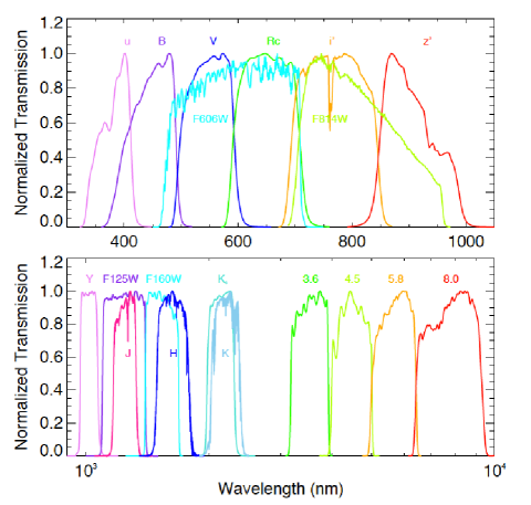
Figure 1.— (Normalized) total system throughput (quantum efficiency) of the optical (top panel), and near to mid-infrared filters (bottom; log scale on x axis) of data available in the UDS CANDELS field.

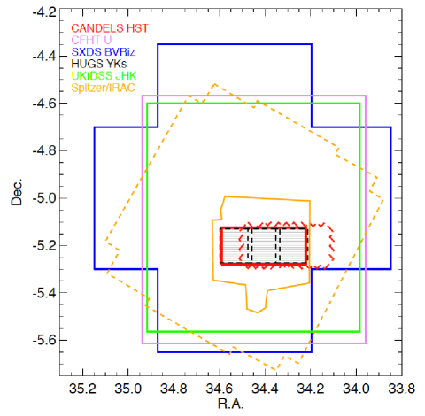
Figure 2.— Coverage of the imaging data in the UDS field: HST WFC3 (red solid and grey hatched region; the detection band for the present multiwavelength catalog) and ACS (red dashed), CFHT $u$-band (purple; Almaini et al. in prep.), Subaru data ($BVR_{c}i^{\prime}z^{\prime}$; blue; Furusawa et al. 2008), UKIDSS ($JHK$; green; Almaini et al. in prep.), HUGS ($YK_{s}$; black dashed; $3$ pointings; Fontana et al. in prep.), Spitzer/IRAC SEDS ($3.6$ and $4.5\mu$m; orange solid; Ashby et al. resubmitted) and SpUDS (four IRAC bands; orange dashed).

2.3. Spitzer/IRAC data

Apart from the shallow ($4\times 30$s) IRAC coverage obtained by the Spitzer Wide-Area Infrared Extragalactic Survey (SWIRE; Lonsdale et al., 2003), the UDS was surveyed as part of a Spitzer cycle-4 Legacy Program: the Spitzer UKIDSS Ultra Deep Survey (SpUDS hereafter; PI: J. Dunlop). SpUDS covers an area of about $1$ square degree (see Figure 2) in the four IRAC channels ($3.6$, $4.5$, $5.8$ and $8.0\mu$m) and reaches a depth of $24.7$ mag ($1\sigma$) at $4.5\mu$m. Images (and SExtractor catalogs) for SpUDS can be found online.

A subregion of SpUDS ($0.40$ deg²; see Figure 2) — that also contains the full CANDELS UDS field — has recently been observed as part of the Spitzer Extended Deep Survey (SEDS hereafter; PI: G. Fazio) during the Spitzer Warm Mission at $3.6$ and $4.5\mu$m. A final UDS mosaic incorporating all coextensive exposures from SEDS, SWIRE and SpUDS was generated by the SEDS team so as to reach the desired $12$ hours total integration time/pixel within the SEDS footprint (Ashby et al., resubmitted). SEDS reaches a point-source sensitivity of $26$ AB mag ($3\sigma$) at both $3.6$ and $4.5\mu$m .

Additional IRAC observations of parts of each SEDS field are now underway as part of the SEDS-CANDELS program (PI: G. Fazio). The S-CANDELS observations of the UDS (PID 80218), when completed, will cover $\sim$150 arcmin² within the CANDELS area and reach a maximum depth of about $50$ hours (four times the existing depth).

2.4. Spectroscopy

A number of spectroscopic observations were conducted in the UDS field. They often targeted specific types of objects: passively evolving galaxies (Yamada et al., 2005), radio sources (Simpson et al. 2006, 2012; Vardoulaki et al. 2008; Akiyama et al. in prep.; Pearce et al. in prep.), QSOs (Smail et al., 2008), Ly$\alpha$ emitters (Ouchi et al., 2008), galaxy cluster members (Geach et al., 2007; van Breukelen et al., 2007; Papovich et al., 2010; Tanaka et al., 2010; Finoguenov et al., 2010).

Extensive spectroscopic campaigns have recently increased the number of known redshifts in the UDS field. A spectroscopic campaign using Magellan/IMACS multi-object spectrograph (PIs: M. Cooper & B. Weiner) provides reliable spectroscopic redshifts for $272$ sources within the CANDELS UDS field of view (Cooper et al. in prep.). The UDSz on-going ESO Large Programme (PI: O. Almaini) is being carried out with the VLT/VIMOS and VLT/FORS2 spectrographs and is obtaining spectra for $\sim 3500$ sources in the full UDS field. Most of these spectroscopic redshifts are still proprietary, however, and will be added to the CANDELS catalog as soon as they become publicly released. At the time of publication, only $210$ sources in the catalog have a non-proprietary spectroscopic redshift.

3. The CANDELS UDS $F160W$-selected catalogue

3.1. $F160W$ detection band

The field of view covered by the $F160W$ data is about $201.7$ arcmin². Exposures are shorter at the eastern end of the mosaic (to accommodate $F350LP$ exposures during the same orbit, see Koekemoer et al. 2011, Figure 17). We estimate the limiting magnitudes as a function of position (from the rms map). They are computed for each pixel rescaled to an area of $1$ arcsec² at a $1\sigma$ level. Figure 3 shows the distribution of the limiting magnitudes across the $F160W$ image and its associated histogram. The peaks in the distribution are found at $27.75$, $28.06$ and $28.30$ and we therefore clearly identify three main areas at different depths: mag $<27.90$ (the $\sim 1/3$ shallower Eastern tiles), $27.90<$ mag $<28.26$ (the $2/3$ deeper Western tiles and tile overlaps in the shallow region) and mag $>28.26$ (tile overlaps in the deeper region) respectively corresponding to regions of about $58.7$, $136.9$ and $5.9$ arcmin². The present catalog also contains for each source an estimation of the limiting magnitude at the position where the source is detected (see §3.3 for details).

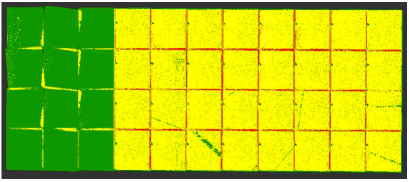
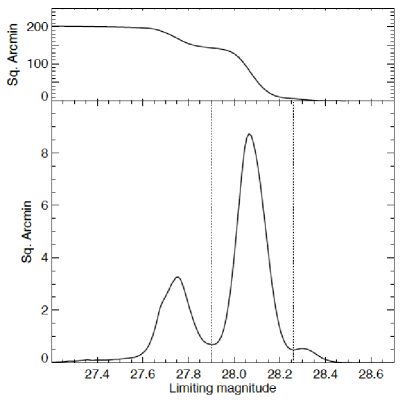
Figure 3.— Limiting magnitudes of the $F160W$ image within an area of $1$ arcsec² square ($1\sigma$). Top: Distribution over the CANDELS UDS field. Regions with limiting magnitudes mag $<27.90$, $27.90<$ mag $<28.26$ and mag $>28.26$ are shown in green, yellow and red respectively. Bottom: Distribution of area with a given limiting magnitude (per bin of $0.01$). The top inset shows the cumulative distribution of area with sensitivity greater than a given limiting magnitude.

3.2. Source extraction

3.2.1 Modifications of the SExtractor software

We used a slightly modified version of the SExtractor software version 2.8.6 (Bertin & Arnouts, 1996) for the source extraction in the $F160W$ image.

(i) Several tests by the GOODS team showed that the ‘inner annulus’ adopted by SExtractor and used for the determination of the local sky background barely reaches the edges of sources (especially for faint sources), resulting in the wings of galaxies being included in the sky measurement and the total SExtractor source flux underestimated. We therefore adopt the same modification of the SExtractor code that ensures that the ‘inner annulus’ is at least $1\arcsec$ radius wide (Giavalisco et al., 2004; Grazian et al., 2006).

(ii) After the detection is performed, SExtractor runs a cleaning process that attempts to merge sources that were falsely split. The original SExtractor cleaning function had a tendency to merge ‘non detection’ sources to a real source close-by. We adopt a modified cleaning routine (i.e. modified clean.c) that ensures that these sources are discarded.

(iii) We also modified SExtractor in various places to ensure that, in dual mode, it uses the gain of the measurement image, and not the detection image, when calculating isophotal-corrected magnitudes.

3.2.2 SExtractor cold and hot detection modes

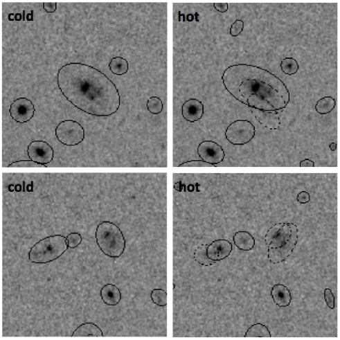
Figure 4.— SExtractor cold and hot modes. Left and right panels respectively show the differences between the cold and hot source extraction modes for two distinct regions (upper and lower panels; $10\arcsec\times 10\arcsec$) of the WFC3 $F160W$ data. SExtractor Kron ellipses are overlaid. The first region is centered on a bright ($H\sim 23$) extended galaxy. The second region contains several clumpy galaxies ($H\sim 25$). In both cases, the faint sources that are only detected in the hot mode have $H\sim 27$.

Traditional wide field surveys were usually not very deep. The source extraction was therefore focussed on deblending bright, extended sources, avoiding for example, the separation of galaxy sub-structures into multiple objects. For deeper surveys, source extraction was usually tuned to push the detection in order to pick up faint and small galaxies. In contrast, recent surveys, and in particular CANDELS, reach unprecedented depth over wide areas. The scientific goals of such surveys extend from the study of nearby sources to the discovery of the farthest and faintest galaxies in the early Universe. It has been unfeasible to find a single setup for the extraction of sources. We therefore need to adapt the detection methodology. Recent works have adopted a rather simple strategy to deal with this issue, using a two-step approach (see e.g.,  Gray et al., 2009, and references therein). First, SExtractor is run in a so-called ‘cold’ mode that extracts and deblends efficiently the brightest sources. It is then run in a so-called ‘hot’ mode optimized for the detection of faint objects. The parameters were further adjusted to obtain a consistent photometry between the cold and hot mode. The adopted SExtractor cold and hot mode parameters are provided in Appendix A.

Figure 4 illustrates the differences between the cold and hot source extraction modes on the $F160W$ image in the vicinity of several extended, clumpy galaxies. The cold mode detects the clumpy galaxy as one single object, merging all the clumps together in one single source, while the hot mode tends to separate clumps into individual objects. Nevertheless, the hot mode detects the faintest objects of the image that were missed by the cold mode. By making use of these two complementary detection modes, we aim at producing the most reliable and complete source catalog possible. SExtractor was run twice to create the cold and hot mode catalogs and associated segmentation maps. The cold and hot mode catalogs contain $27167$ and $37715$ sources respectively.

3.2.3 Cold + Hot combination routine

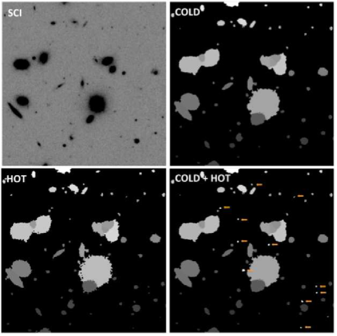
Figure 5.— Cold + hot combination routine. Panels respectively show a region of $40\arcsec\times 40\arcsec$ of the $F160W$ image (‘SCI’; top left), the SExtractor segmentation map for the cold mode (‘COLD’; top right) and the hot mode (‘HOT’; bottom left) and the cold + hot combined segmentation map (‘COLD + HOT’; bottom right). The shades of grey correspond to the source identification number in the SExtractor catalogs. The orange arrows, in the bottom right panel, indicate sources that were only detected in the hot mode and added to the cold mode catalog.

The cold and hot catalogs were merged. The adopted cold + hot combination routine was adapted from GALAPAGOS, a software designed for source extraction, light-profile modeling and catalog compilation of large astronomical surveys (see Barden et al. 2012 and the GALAPAGOS manual for details).

The combined cold + hot catalog includes all the sources detected in the cold mode + the sources detected in the hot mode at positions where no cold source was detected. In short, for each source in the hot mode, the routine checks whether it falls within the Kron ellipse of a cold mode detected source. If it does, the source is ignored. The final merged catalog therefore contains the full cold mode catalog followed by the ‘hot mode only’ sources (with new updated identification indices).

For example, in Figure 4, the routine will consider the different clumps of the extended galaxies as part of the same object — because they are all detected within the same Kron ellipse in the cold mode — and therefore appear as one unique object (one line) in the merged catalog (whose SExtractor characteristics are reproduced from the cold mode catalog). Sources that are only detected in the hot mode and isolated (i.e., not within a Kron ellipse of a cold mode source) are simply added to the catalog with the SExtractor measurements of the hot mode catalog.

Figure 5 shows a region of the $F160W$ image with the SExtractor segmentation maps of the cold, hot, and cold + hot modes. In the final combined segmentation map, the isophotal areas for sources detected in the cold mode are directly reproduced from the cold mode segmentation map. The isophotal areas for sources only detected in the hot mode are then added with their new identification number from the cold + hot merged catalog.

The final combined $F160W$-selected catalog contains $35932$ sources. Figure 6 shows the source number counts (per bin of $0.5$ mag; also listed in Table 2) with the contributions of the cold and hot mode overlaid. The flux densities and uncertainties in the $F160W$-band reported in the multiwavelength catalog correspond to the SExtractor outputs FLUX_BEST and FLUXERR_BEST, converted into $\mu$Jy using the Koekemoer et al. (2011) zeropoints.

The completeness limit of the UDS $F160W$ catalog was estimated by comparing with deeper data in the GOODS-South field. The central part of this field was observed in $10$ epochs (Grogin et al. 2011) i.e., five times the depth of UDS. We ran SExtractor (cold + hot) on the 10-epoch GOODS-S combined $F160W$ mosaic and derived number counts similarly to the UDS. By comparing number counts in GOODS-S Deep with UDS, we estimate that the $90$% ($50$%) limit of completeness of the UDS $F160W$ data is $26.70$ ($27.05$).

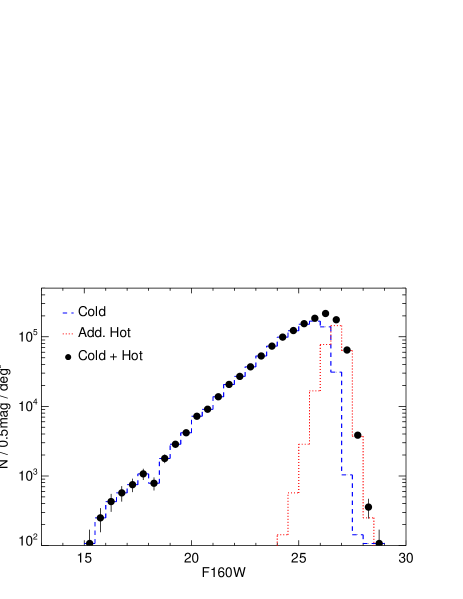
Figure 6.— Source number counts in the F160W band (black dots). Blue dashed and red dotted histograms respectively show the contribution of the cold and hot mode. We assume Poissonian error bars.

Table 2Number counts in the CANDELS UDS $F160W$ image

Mag	N mag-1 deg-2a
$15.75$	$250\pm 94$
$16.25$	$428\pm 124$
$16.75$	$571\pm 143$
$17.25$	$749\pm 164$
$17.75$	$1071\pm 195$
$18.25$	$785\pm 167$
$18.75$	$1784\pm 252$
$19.25$	$2855\pm 319$
$19.75$	$4176\pm 386$
$20.25$	$7209\pm 507$
$20.75$	$9101\pm 570$
$21.25$	$13740\pm 700$
$21.75$	$20664\pm 859$
$22.25$	$26946\pm 981$
$22.75$	$36974\pm 1149$
$23.25$	$53070\pm 1376$
$23.75$	$73449\pm 1619$
$24.25$	$99003\pm 1880$
$24.75$	$122950\pm 2095$
$25.25$	$154357\pm 2347$
$25.75$	$184443\pm 2566$
$26.25$	$216207\pm 2778$

• Uncertainties on the number counts are Poissonian.

3.3. Additional $F160W$-related values

$\bullet$ $F160W$ Limiting magnitude: For each source in the catalog, we derive a limiting magnitude indicating the depth of the $F160W$ image in the region where the source falls. This limiting magnitude is derived from the square root of the average of the rms squared in the SExtractor segmentation map of each source scaled to an area of $1$ arcsec². In practice, the limiting sensitivity in $HST$ images depends on the source size, and faint galaxies can be significantly smaller than $1$ arcsec² and thus be detected fainter than this fiducial magnitude limit. The knowledge of the depth fluctuation of the detection image is fundamental for any future volume-sensitive statistics (e.g., luminosity functions etc.).

$\bullet$ Flag: Not all objects detected by SExtractor are real. For example, SExtractor typically detects spurious sources in the spikes of very bright stars. Some sources also fall at the edges of the detection image where the photometry is not optimal. A flag column is therefore included in the catalog which indicates star spikes and bright halos as well as large artifacts and noisy edges (see Appendix B for details).

4. Photometry of the HST data

The photometry of the other HST bands (i.e., WFC3 $F125W$, ACS $F606W$ and $F814W$) was derived using SExtractor in dual-mode with a source detection on the $F160W$ image. To take into account the PSF differences between the F160W detection image and the $F125W$, $F606W$ and $F814W$ images, these measurement images are PSF-matched to the $F160W$ data. Empirical PSFs were derived from stacking the images of several isolated and unsaturated stars in the field. In order to provide a more accurate description of the central region, we replaced the inner-most pixels (within a radius of 3 pixels from the center) with a simulated PSF generated with the TinyTim package (Krist 1995). The TinyTim PSF was dithered and drizzled in the same manner as the observations, and normalized such that the total flux of the newly constructed hybrid PSF model is the same as that of the stacked star. We found this hybrid PSF accurately reproduced the growth curves of stars out to $3$″. Further details on the PSF models can be found in van der Wel et al. (2012). Using iraf/psfmatch, we generated matching kernels from these hybrid PSFs, replacing the high-frequency and low signal-to-noise components of the PSF matching function with a model computed from the low frequency and high signal-to-noise components. Similarly to the $F160W$ catalog, SExtractor was then run twice for each band to create the cold and hot-mode catalogs that were then merged.

Part of the $F160W$ field of view (i.e., the eastern $\sim 1/4$ of the CANDELS UDS field; see Figure 2) was not covered by ACS. For sources detected in $F160W$ but outside the ACS field of view, we set the flux density and uncertainties for $F606W$ and $F814W$ to $-99$.The region covered by both WFC3 and ACS is about $154$ arcmin².

Although commonly adopted Kron magnitudes (SExtractor MAG_AUTO) are mainly consistent with isophotal magnitudes for bright or faint isolated sources, they are usually estimated over areas larger than isophotal ones therefore resulting in a lower signal-to-noise. They can also be contaminated by neighboring sources. In high-resolution data such as HST, the isophotal area tends to follow more precisely the apparent size of the sources. Using isophotal magnitudes also guarantees that the flux is derived in the same area as the isophotal area defined by SExtractor for the $F160W$ image. For these reasons, isophotal magnitudes were adopted in past multiwavelength catalogs such as the GOODS-MUlticolor Southern Infrared Catalog (GOODS-MUSIC; Grazian et al. 2006), a multiwavelength catalog (visible to mid-infrared) that covers $143.2$ arcmin² in the GOODS-South field. Following these past works, we adopt isophotal colors for all sources assuming that the ratio of FLUX_BEST $/$ FLUX_ISO fluxes represents the aperture correction to total flux in F160W, and apply this uniformly to all HST bands. SExtractor isophotal flux densities (FLUX_ISO) and flux uncertainties (FLUXERR_ISO) for $F125W$, $F606W$ and $F814W$ were first converted into $\mu$Jy using Koekemoer et al. (2011) zeropoints and then into total flux densities following:

$F(\lambda)=F_{Iso}(\lambda)\times F_{Best}(160)/F_{Iso}(160)$
$F_{unc}(\lambda)=F_{unc;Iso}(\lambda)\times F_{Best}(160)/F_{Iso}(160)$

5. Photometry for the ground-based and Spitzer images

It has always been challenging to derive reliable photometry for multiwavelength imaging surveys, which combine data with a large variety of survey depth and resolution. The CANDELS UDS field is a typical example, covered by both high-resolution HST data and lower resolution ground-based and Spitzer/IRAC data. Figure 7 shows the same region of the CANDELS UDS field in HST $F160W$, VLT/HAWK-I $Y$, the Subaru $B$-band and Spitzer/IRAC SEDS $3.6\mu$m. The field of galaxies can appear to be quite different through different bands, due to their varying colors, the different depths of the data sets, and particularly the different PSFs. Close neighbors that appear isolated in high resolution data can appear strongly blended at lower resolution. It is therefore crucial to be able to deblend these sources from their projected neighbors.

Several efforts were conducted to overcome these issues with the development of optimized photometry software (e.g., ConvPhot; de Santis et al., 2007). In the present work, we make use of the template-fitting photometry software TFIT, for consistency with the other CANDELS multiwavelength catalogs (e.g., Guo et al. submitted for GOODS-S), to derive the photometry for all the non-HST data. TFIT has the advantage of using shifted kernels to account for any remaining small image distortion in the low-resolution images. It also works on original pixel scale of the low-resolution image. Laidler et al. (2007) and Papovich et al. (2001) provide a complete description of the TFIT software and Lee et al. (2012) present a set of simulations that validate this template-fitting technique and quantify its uncertainties. We only summarize the main steps in the following. In brief, TFIT uses a-priori information on the position and surface brightness profile of sources measured on a high resolution image (in the present work, the $F160W$-band) as priors to derive their corresponding photometry in lower-resolution images. As mentioned earlier, one of the main reasons for using TFIT is to derive reliable photometry for sources that overlap in the low-resolution image. TFIT uses information from their high-resolution (often well separated) counterparts and fits them simultaneously. First, TFIT builds a low resolution (normalized) template model of each source by smoothing the high resolution image of the object to the PSF of the low-resolution image using a convolution kernel. The best fit fluxes to the low resolution image are then derived from these templates using chi-square minimization.

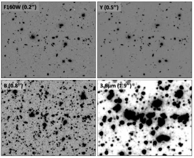
Figure 7.— $2\arcmin\times 1\farcm 5$ region of the CANDELS UDS field seen in four of the bands available (from high to low-resolution data): the CANDELS HST $F160W$ (top left), VLT/HAWK-I $Y$ (top right), the Subaru $B$-band (bottom left) and Spitzer/IRAC SEDS $3.6\mu$m (bottom right). The FWHM of each band is also indicated (in parentheses). This particular crowded region of the UDS field hosts a galaxy cluster at $z=0.65$ (Geach et al., 2007).

5.1. Preparing the low-resolution images

TFIT requires a careful preparation of the low-resolution images.

$\bullet$ Astrometry: The low-resolution images should also have a compliant astrometry with the high-resolution images. The pixel scale of the low-resolution image should be equal to (or an integer multiple of) the pixel scale of the high-resolution image. All ground-based images were resampled to the $F160W$ pixel scale of $0.06$″and aligned to the CANDELS HST data astrometry using swarp (Bertin, 2010). We keep the original pixel scale ($0.6$″) of the Spitzer data (SEDS, SpUDS). The astrometry of SEDS (Ashby et al. resubmitted) is compliant to the astrometry of the HST images so no realignment was needed. This was not the case for the SpUDS data that were therefore reprojected to the HST astrometry also using swarp.

$\bullet$ Background subtraction: The low-resolution images first need to be background-subtracted. For each image, a first rough background approximation was determined by smoothing the image on large scales using a large-annulus ring-median filter and then subtracted from the image. The image was then smoothed to the corresponding image PSF scale and sources were masked. To account for the wings of the sources, the source masks were enlarged by convolving with a Gaussian kernel. Several iterations were performed, starting from the brightest sources with high signal-to-noise (S/N) ratio down to sources with a S/N$\sim 5$ above the mean background. The non-masked pixels were used to create a ‘noise’ map, which was interpolated to determine the background in the masked pixels.

We tested the background subtraction routine by sampling the noise in the background-subtracted low-resolution images. We randomly added $1000$ artificial sources in the $F160W$ image (privileging regions without sources) and derived the photometry of their non-existent counterparts in the low-resolution images. We expect the S/N (flux density over uncertainty) to be a Gaussian, centered to zero with $\sigma=1$. The background subtraction technique works well for ground-based data.

For IRAC data, however, both the mean S/N and the TFIT residual image (see §5.4) are found to be slightly negative ($\sim 10^{-4}$ MJy/sr) i.e., the routine is over-subtracting the background. Although this quantity is negligible for bright objects, it becomes dominant for faint sources. We therefore implemented an additional background correction for the IRAC data. We ran TFIT on the background-subtracted images, subtracted the TFIT output collage — an image of the sources as modeled by TFIT — and repeated the background subtraction procedure. We then repeated the test with artificial sources and found a Gaussian-like distribution of the S/N and mean residuals $<10^{-6}$ MJy/sr). TFIT was run a fourth time on the final image.

5.2. Preparing kernels and PSF

One of the key processes within TFIT is the smoothing of the high resolution detection image to the PSF of the lower resolution measurement image. Such a smoothing process is performed by applying a convolution kernel. The derivation of the convolution kernel is not done by TFIT and must be provided beforehand by the users.

Several techniques have been developed to derive an accurate convolution kernel, in particular those by Alard & Lupton (1998) and Alard (2000). In the case of the UDS visible and near-infrared ground-based data, we adopt a slightly simpler method based on analysis in the Fourier space, similar to the convolution kernel derivation technique presented in Aniano et al. (2011). Such method can be implemented with standard astronomical tools for image analysis and has been successfully used for the GOODS-MUSIC (Grazian et al., 2006; Santini et al., 2009) and GOODS-ERS database (Santini et al., 2012). In brief, we first derive the PSFs of the detection and measurement image, $PSF_{1}$ and $PSF_{2}$ respectively, e.g., by summing up stars in the field.These two PSFs are then normalized. The convolution kernel $K$ is, by definition:

$$PSF_{2}(x,y)=K(x,y)\otimes PSF_{1}(x,y)$$ (1)

The derivation of the exact shape of the convolution kernel is done in the Fourier space i.e. if ${\aleph}=FT(K)$, ${\wp}_{1}=FT(P_{1})$ and ${\wp}_{2}=FT(P_{2})$, the Fourier transform of the kernel is given by:

$${\aleph}=\frac{{\wp}_{2}}{{\wp}_{1}}$$ (2)

A low passband filter (LPBF) was applied in the Fourier domain to remove the effects of noise and suppress the high frequency fluctuations. A residual was computed from the two PSFs in order to check for the validity of the derived filter. Finally, ${\aleph}$ was transformed back to the pixel space and normalized to unity (to preserve the flux of the objects) following:

$$K(x,y)=FT^{-1}({\aleph}\cdot LPBF)$$ (3)

If the high and low-resolution images have significantly different resolutions — such as HST and Spitzer — the PSF of the low-resolution images can be used directly as the convolution kernel. For IRAC, we obtained a set of $5\times$ spatially-oversampled PSFs (W. Hoffman; private communication; see also IRAC Data Handbook, Appendix C). There are $25$ such oversampled PSFs for each channel, representing a $5\times 5$ sampling across the detector to map PSF variation. We averaged together these $25$ location-specific PSFs to construct a single, location-averaged, PSF for each channel. The SEDS and SpUDS images are mosaics of a series of Astronomical Observation Requests (AOR; $107$ and $26$ respectively) that were executed with different PAs. The model PSF is rotated by the PAs for each AOR. The average of all rotated PSFs is then smoothed by a boxcar kernel, a mandatory step because the model PSF is sharper than the true IRAC PSF. Tests on the SEDS and SpUDS data showed that the optimal smoothing is obtained using a boxcar size of $23$ pixels ($0.06\arcsec$/pixel). Finally, the smoothed PSF are circularized by putting the pixels outside a diameter of $25\arcsec$ to zero and normalizing the total ‘flux’ in the template to unity.

5.3. Preparing TFIT input source catalog and segmentation map

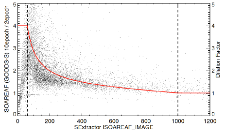
Figure 8.— Ratio between the $F160W$ SExtractor ISOAREAF_IMAGE of sources in GOODS-South CANDELS Deep ‘10Epoch’ (i.e. full CANDELS Deep image) and ‘2Epoch’ (i.e., after the two first CANDELS epochs) in function of the ISOAREAF_IMAGE of the ‘2Epoch’ (black dots). Also plotted are the dilation factor correction (red line) depending on a given source isophotal area (vertical dashed lines; see §4.3.2).

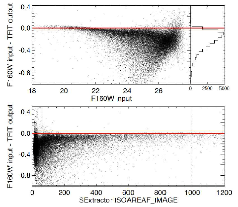
Figure 9.— TFIT output photometry derived from the $F160W$ image smoothed to a resolution of $0.4\arcsec$ (i.e., to the resolution of the HAWK-I data): Top: versus the $F160W$ initial photometry (SExtractor MAG_BEST). The histogram of the distribution is plotted in the right inset Bottom: versus the isophotal area (SExtractor ISOAREAF_IMAGE). The vertical dotted lines mark the positions for ISOAREAF_IMAGE $=60$ and $1000$ that will be relevant for our dilation correction (see §5.3.2). TFIT fluxes are gradually underestimated for fainter and/or smaller sources.

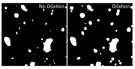
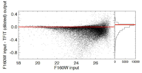
Figure 10.— Dilation correction. Top: Portion of the segmentation map before (left panel) and after dilation (right). Isophotal area larger than $1000$ pixels are not dilated whilst smaller areas are dilated according to the adopted correction (see text and Figure 8) Bottom: Same as Figure 9 but providing TFIT with SExtractor dilated input segmentation map. The TFIT output is now much more consistent with the $F160W$ input photometry thanks to the implemented dilation correction.

In order to derive photometry, TFIT uses as the source template only pixels within a segmented region. In past works using TFIT (e.g. Laidler et al. 2007), this region was defined by the SExtractor segmentation map. This implies that only pixels within the HST isophotal area were used to construct templates for TFIT. However, past studies (e.g. De Santis et al. 2007) have shown that SExtractor tends to underestimate the size of the source isophotal areas especially for faint and/or small sources and that therefore part of the source flux was missed. Unfortunately, it is challenging to estimate how much of the flux is missed exactly because (i) we do not know how much flux is actually outside the segmented region for each source, and (ii) a portion of this flux will be considered as background in the preparation of the low-resolution images for TFIT. The size of the isophotal area depends on the threshold adopted in the detection image. However, for faint sources, a significant fraction of their flux probably falls below the isophotal detection threshold. This isophotal area is fed as an input parameter to TFIT which, as a consequence, tends to miss a significant fraction of the flux and underestimate the total magnitude. We run a series of tests to quantify how SExtractor underestimates the isophotal area and implement a ‘dilation’ correction to compensate for this underestimation. This issue mostly concerns sources that are either faint or with a small isophotal area, two populations that are overlapping as size strongly correlates with brightness. We will interchangeably refer in the following sections to faint/bright or small/large sources.

5.3.1 SExtractor estimation of source isophotal area

The following tests were done on the $F160W$ band since it is the catalog detection band and the reference high-resolution image for our TFIT run.

As mentioned in §3.2.3, the central part of the GOODS-South field was observed in ten epochs, five times the UDS depth. We ran SExtractor (‘cold + hot’ then merged) on the full GOODS-S $F160W$ image (’10Epoch’) and also on an image made only from the first two epochs (‘2Epoch’). Figure 8 shows the ratio of ISOAREAF_IMAGE parameter between the ‘10Epoch’ and ‘2Epoch’ images. SExtractor derives larger source isophotal areas (ISOAREAF_IMAGE, the number of pixels above the adopted threshold) in the deeper image. As expected from previous studies, the isophotal area is smaller in the shallower image for faint sources. Although SExtractor nicely recovers the total ISOAREAF_IMAGE for bright sources (ISOAREAF_IMAGE $>1000$ pixels), it gradually loses part of the source for fainter objects with an underestimation of at least a factor of $4$ for sources with ISOAREAF_IMAGE $=60$ pixels.

As a test of how isophotal area affects photometry, we smoothed the $F160W$ image to the 0$\farcs$4 resolution of the VLT/HAWK-I data by convolving the image by the corresponding kernel. Using this same kernel, we ran TFIT, intending to recover the input photometry of the original (unsmoothed) $F160W$ image. Figure 9 shows the difference between the output of TFIT and the input $F160W$ magnitude versus input magnitude (top) and SExtractor isophotal area (bottom; i.e. the ISOAREAF_IMAGE parameter). Figure 9 shows that the TFIT output is in good agreement with the $F160W$ input values for bright sources ($mag_{F160W}<20$ and ISOAREAF_IMAGE $>1000$ pixels) but worsens rapidly with faintness (and smaller isophotal area) with an average offset of $-0.24$ for $26<mag_{F160W}<27$ ($-0.26$ for sources with ISOAREAF_IMAGE $<60$ pixels). As expected, SExtractor tends to underestimate the isophotal area of sources and therefore TFIT fails to recover the expected input photometry for faint objects. Smoothing the $F160W$ data to match even lower-resolution data e.g., $0.8\arcsec$ (Subaru/Suprime-Cam) or Spitzer/IRAC gives trends similar to those of Figure 9, although the discrepancies between input and TFIT output are less dramatic with an average offset of $-0.1$ for $26<F160W<27$.

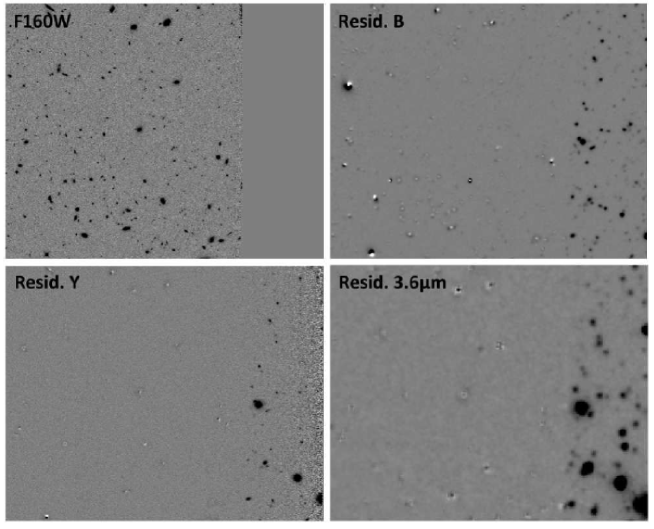
Figure 11.— $2.5\arcmin\times 1.5\arcmin$ sub-region of the TFIT residual output images. The first panel shows the $F160W$ detection image. We deliberately choose the edge of the $F160W$ field of view to visually assess the effect of the source removal by TFIT in the $B$-band (top right), the $Y$-band (bottom left) and SEDS $3.6\mu$m band (bottom right).

5.3.2 Dilation correction

In order to deal with this particular issue, we adopt a correction technique similar to the one implemented within the ConvPhot software. ConvPhot automatically dilates the area of every source on the segmentation map generated by SExtractor. Sources with an area above a minimum threshold ($m_{(AREA)}$) are dilated by a constant factor of $4$ (i.e., doubling the area). Sources smaller than $m_{(AREA)}$ are dilated to reach this minimum threshold. The dilation correction is done using a publicly available routine called dilate (see  de Santis et al., 2007). dilate expands the segmentation map by a fixed factor but prevents the merging between close sources.

We refine this dilation technique by modifying the dilate routine to adapt it to the present dataset. As observed in Figure 9 (as well as in Figure 8), TFIT recovers well the photometry of sources with ISOAREAF_IMAGE $>1000$ pixels with a difference between the input and TFIT output magnitude of less than $<0.01$. We therefore do not apply any dilation for these sources. The largest discrepancies are obtained for sources with an isophotal area smaller than $60$ pixels (with an underestimation of a factor of $4$ of the isophotal area in the case of GOODS-South ‘2Epoch’/‘10Epoch’ comparison). We therefore adopt a constant dilation factor of $4$ for sources with ISOAREAF_IMAGE $<60$ pixels. As observed in Figure 8, the loss of isophotal area by SExtractor can be parametrized by an hyperbola. We therefore opt for a smooth transition for sources with $60<$ ISOAREAF_IMAGE $<1000$. To summarize, we adopt the following dilation factor corrections:

$\bullet$ If ISOAREAF_IMAGE$>1000$: Dilated_area$=$area
$\bullet$ If $60<$ ISOAREAF_IMAGE $<1000$:
Dilated_area $=-0.0004\times$ area${}^{2}+1.25\times$area $+166$.
$\bullet$ If ISOAREAF_IMAGE$<60$: Dilated_area$=4\times$area

Figure 8 shows the adopted dilation correction. Figure 10 shows its effect on the segmentation map. It also shows the final discrepancies between the input $F160W$ photometry and the TFIT output after dilation. The adopted dilation correction permits us to recover, with more accuracy, the $F160W$ input photometry.

This dilated segmentation map (and updated input source catalog) is adopted for all the TFIT runs on the low-resolution data (ground-based and Spitzer/IRAC data).

5.4. TFIT

TFIT incorporates a procedure that quantifies any small geometric distortions and shifts that could persist even after a careful alignment of the high- and low-resolution images and creates a series of shifted kernels based on these distortions (as part of the ‘registration dance’ stage; see  Laidler et al., 2007, for details). We ran TFIT a second time with these kernels in order to improve the alignment of the model with the data. The shifts are typically less than $0.1$ arcsec for ground based data and less than $0.3$ arcsec for the Spitzer images. For background-subtraction purposes described in §5.1, TFIT was run a third time on the IRAC data.

TFIT produces a residual image derived by subtracting the model image – a collage of the source template scaled by the TFIT flux measurement — from the low-resolution image. The residual image permits us to visualize any TFIT problem such as a non-optimal convolution kernel. Objects that are detected in a low-resolution image but are not in the input catalog derived from the high-resolution data also remain unchanged on this residual image. Residual images of the TFIT second pass are shown in Figure 11 for the $B$, $Y$ and SEDS $3.6\mu$m.

We finally convert the TFIT output into $\mu$Jy using the low-resolution image zeropoints.

6. Combining the final multiwavelength catalog

The final catalog is built by combining the SExtractor HST and TFIT ground-based/Spitzer catalogs. It contains $35932$ sources ($34912$ with a flag $=0$) and $46$ columns. The catalog header is provided in Appendix B.

$\bullet$ Sources that fall on bright star spikes and halos in the Subaru data or the UKIDSS $JHK$ data are assigned a flux density and uncertainty of $-99$.

$\bullet$ The UKIDSS data suffer from cross-talk which echoes all objects in the adjacent amplifiers of each chip. In the $J$-band image, the crosstalk is clearly visible against the background for sources brighter than $J<16.5$. The crosstalk replica on the adjacent channel was shown to have intensity up to 1% of the flux of the original source that drops to about 0.05% beyond the third amplifier (e.g.,  Dye et al., 2006). However, crosstalk produced by fainter sources remains unidentified and could affect the photometry of some sources. Almaini et al. (in prep.) provide further analysis of crosstalk in the UKIDSS data. The crosstalk manifests itself as a spurious ‘image’ that can have different profiles (e.g., a ring-like shape or a positive-negative source, depending if the original object is saturated or not) but often presents a strong negative component. In the present catalog, the regions that were strongly affected by crosstalk were identified on the bluer band ($J$) — where the crosstalk is more prominent — by detecting its negative component using SExtractor on the inverted image (then cleaned by eye to avoid abusive flagging). The most strongly-affected $98$ sources are assigned a flux density and uncertainty in the $J$, $H$ and $K$ bands of $-99$.

$\bullet$ The $3.6$ and $4.5\mu$m photometry listed in the present catalog was derived from the SEDS mosaics. Photometry was also derived from the shallower SpUDS-only $3.6$ and $4.5\mu$m data for checks but not included to avoid redundancy.

$\bullet$ We cross-match the source catalog with $210$ (non proprietary) spectroscopic redshifts in the CANDELS UDS field (see column #45). We also indicate the origin (article published or in preparation) of the spectroscopic redshift as well as the nature of the source when available (see column #46). The abbreviations used in column #46 are detailed in Appendix B.

$\bullet$ Simpson et al. (2006) presented a catalog of $505$ radio-sources from radio imaging of the SXDS with the Very Large Array (VLA). $38$ sources fall within the CANDELS UDS field. We cross-match the VLA catalog with the $F160W$-selected catalog, using a matching radius of $0.5$ arcsec, and found that $36$ VLA sources have a clear $F160W$ counterpart. Likewise, Ueda et al. (2008) listed $1245$ X-ray detected sources ($1213$ point sources and $32$ extended source candidates) in the SXDS field. $32$ point sources (and $2$ extended sources) fall within the CANDELS field of view with $27$ of them having an unambiguous $F160W$ counterpart (matching radius of $1.5$ arcsec). We specify the radio and/or X-ray nature for these sources in column #46.

7. Validation tests on photometry

7.1. Consistency checks for similar filters

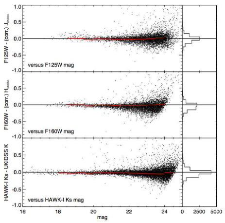
Figure 12.— Comparison of photometry for similar bands: Top: between SExtractor $F125W$ and TFIT UKIDSS $J$ (versus $F125W$). Middle: between SExtractor $F160W$ and TFIT UKIDSS $H$ (versus $F160W$). Bottom: between TFIT HAWK-I $K_{s}$ and TFIT UKIDSS $K$ (versus HAWK-I $K_{s}$). Color corrections were applied in the two upper panels to take into account the filter differences between WFC3 and UKIRT. We only plot sources with S/N $>10$. The histograms of the distributions are shown in the right insets. The red lines show the $\sigma$-clipped mean per bin of $0.5$mag.

$\bullet$ $J$ and $H$ bands: Figure 12 shows the comparison between the HST/WFC3 ($F160W$, and $F125W$) and UKIDSS DR8 ($J$ and $H$) photometry. The WFC3 and UKIDSS WFCAM filters are slightly different (see Figure 1). In order to account for the discrepancy between filters, the UKIDSS flux densities are converted to the WFC3 photometric system using the color corrections adopted by Koekemoer et al. (2011): $F125W=J+0.05(J-H)$ and $F160W=H+0.25(J-H)$. In Figure 12, we only plot sources with $S/N>10$ and $F160W$ CLASS_STAR$<0.98$ to avoid bright (possibly saturated) stars. The agreement is good and shows no systematic offset (i.e., no zeropoint issue) or trends.

$\bullet$ $K$ bands: Similarly, we compare the HAWK-I $K_{s}$ and UKIDSS $K$ photometry (see Figure 12). No correction is applied because the filters are consistent and correction would be negligible. We also find a good agreement between the two bands with no specific discrepancy.

7.2. Validation tests on colors

We study the (optical to near-infrared) colors of stars in the catalog. We first isolate stars in the multiwavelength catalog by selecting sources that have CLASS_STAR $\geq 0.98$. We build a library of synthetic models of stars from the Bruzual-Persson-Gunn-Stryker Atlas of stars (Gunn & Stryker 1983) that we convolve with the response curves of the different filters. We then compare their colors to the colors of the stars in the catalog and derive a series of color-color diagrams; figure 13 shows four of these diagrams. The agreement is excellent.

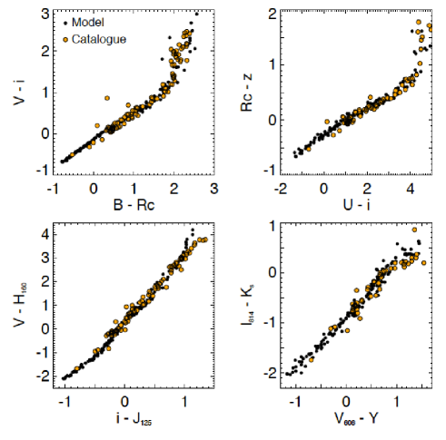
Figure 13.— Color-color diagrams for synthetic models of stars (black dots) and sources from the catalog with CLASS_STAR $>0.98$ (orange dots): clockwise from top left: ($V-i^{\prime}$) vs ($B-R_{c}$), ($R_{c}-z$) vs ($U-i$), ($I_{814}-K_{s}$) vs ($V_{606}-Y$) and ($V-H_{160}$) vs ($i-J_{125}$).

We also look at the distribution of the sources in a $BzK$ color-color diagram (introduced by Daddi et al. 2004) which preferentially isolates $z>1.4$ galaxies. Figure 14 shows the $BzK$ diagram derived from the catalog (using the $K$-band photometry from the UKIDSS DR8 data). Small corrections were applied to account for the differences in filters between UDS and Daddi et al. 2004. Sources with CLASS_STAR $>0.98$ (orange dots) are, as expected, preferentially found in the stellar locus of such diagrams (Daddi et al., 2004). All (but one) sources with spectroscopic redshift $1.4<z_{spec}<2.5$ (red squares) are s$BzK$-selected galaxies (within error bars) i.e., have $BzK\geq-0.2$ (where $BzK=(z-K)-(B-z)$) and therefore lie in the typical locus of star-forming galaxies at $1.4<z<2.5$. The only source not s$BzK$-selected is found in the locus of p$BzK$-selected galaxies ($BzK<-0.2$ and $z-K>2.5$) i.e., has colors consistent with a passive galaxy at $1.4<z<2.5$.

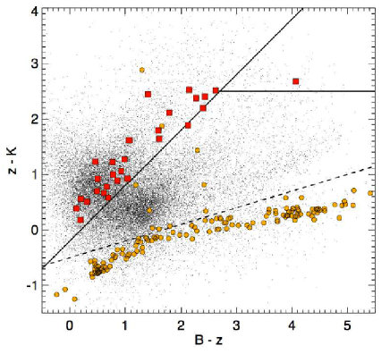
Figure 14.— $BzK$ color-color diagram of the UDS catalog for sources with S/N$>3$ in $B$, $z$ and $K$. Color corrections were applied to the $z-K$ and $B-z$ colors to account for the differences in filters between UDS and Daddi et al. 2004. Sources with CLASS_STAR $>0.98$ are shown by the orange dots and are found preferentially in the Daddi et al. (2004) locus for stars i.e. have $(z-K)<0.3\times(B-z)-0.5$ (below the dashed line). Sources with spectroscopic redshift $1.4<z_{spec}<2.5$ are shown by the red squares. All but one have colors consistent with star-forming galaxies at $1.4<z<2.5$ (s$BzK$-selected galaxies i.e., lie above the non-horizontal solid line). The exception lies in the p$BzK$ selection area i.e has colors consistent with passive elliptical galaxies at $1.4<z<2.5$.

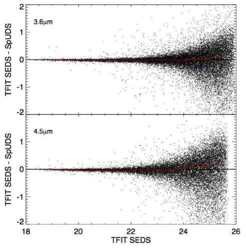
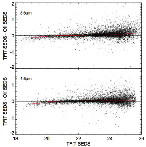
Figure 15.— Comparison between the TFIT SEDS photometry and TFIT SpUDS-only (top) and the (StarFinder) SEDS-UDS catalog (bottom) at $3.6$ and $4.5\mu$m for sources with S/N $>3$. The red lines show the $\sigma$-clipped mean per bin of $0.5$mag.

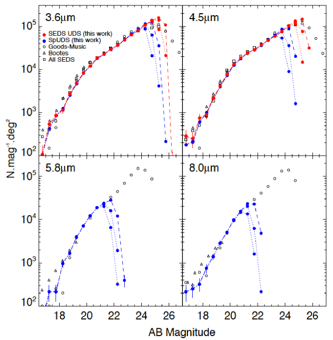
Figure 16.— Source number counts (stars and galaxies) in the four IRAC bands: $3.6\mu$m (top left), $4.5\mu$m (top right), $5.8\mu$m (bottom left) and $8.0\mu$m (bottom right). The counts derived from the present catalog (in bin of $0.5$ mag) are shown by the colored dots for SEDS (red) and SpUDS-only (blue). We adopt Poissonnian errors on the counts. The multiple curves show the counts for different cuts in signal/noise: S/N = $3$ (dashed line) and S/N = $4$, $5$ (dotted lines from right to left). Published number counts from Fazio et al. (2004) (in the Boötes field) and Ashby et al. (resubmitted; for the full SEDS survey) are shown in open symbols (triangles and squares respectively). Counts derived from the GOODS-MUSIC are overplotted in open circles.

7.3. Spitzer/IRAC photometry

As mentioned earlier, we also derive TFIT photometry for the SpUDS-only $3.6$ and $4.5\mu$m images. Figure 15 shows the comparison between the TFIT photometry for the SEDS and SpUDS IRAC data. The agreement is good with no systematic offset and no suspicious trend with magnitude — i.e., the difference is fairly symmetric at a given magnitude — suggesting that there is no zeropoint offset and no systematic background subtraction issue that could bias the faint sources either in the SEDS or the SpUDS mosaics.

We also compare our TFIT SEDS photometry to the (StarFinder) SEDS catalog (Ashby et al. resubmitted). We made use of an early distribution of their catalog to the CANDELS group (SEDS team; private communication) and cross-matched their source list with our $F160W$-selected catalog. In the SEDS data, confusion limit is an issue and it is therefore important to use a small aperture in order to avoid flux contamination from the wings of nearby sources. We therefore compare the TFIT SEDS photometry to their aperture-corrected StarFinder photometry derived in a $2.4^{\prime\prime}$ diameter aperture. The agreement is good. The discrepancy increases at faint magnitudes since StarFinder does not deblend faint sources. Their photometry may be contaminated by neighboring objects and over estimated hence the positive offset. At the bright end (mag $<20$), stars have magnitudes consistent in both catalogs. Bright galaxies however show a larger discrepancy. This was expected when considering magnitudes derived in such a small aperture. The match between TFIT SEDS and StarFinder is excellent for bright galaxies ($<0.1$ mag) when using the StarFinder $6^{\prime\prime}$ diameter aperture-corrected photometry.

Figure 16 shows the source number counts derived from the present catalog in the four Spitzer/IRAC bands (SEDS UDS in red and SpUDS-only in blue). Counts are derived for different cuts in signal-to-noise (S/N $=3,4,5$) since IRAC photometry at lower S/N becomes rapidly unreliable and strongly biased by background contamination issues. We therefore strongly advise users to regard the IRAC flux density estimates for sources with S/N $<3$ with caution. Published source number counts from Fazio et al 2004 in the Boötes field and from Ashby et al. (resubmitted) derived from the full SEDS survey (M. Ashby, private communication) are overplotted for information. We also derive IRAC number counts from GOODS-MUSIC. We precise that the GOODS IRAC $5.8$ and $8.0\mu$m data (shown here as the open points) are much deeper than the SpUDS data.

Our IRAC source number counts are in good agreement with previously published number counts. As mentioned earlier, the SpUDS data for $3.6$ and $4.5\mu$m are included in the SEDS mosaic, although here we measure the photometry independently from a different TFIT run on the SpUDS images alone. The number counts are in perfect agreement up to the completeness limit of the SpUDS data i.e., about $1.5$ mag brighter than the SEDS UDS data. The agreement is also excellent with both the GOODS-MUSIC and the full SEDS survey (that also includes the present SEDS UDS data). As expected, the full-SEDS number counts (derived from the SEDS StarFinder aperture photometry catalog) fall below our TFIT SEDS UDS counts (starting $0.5$ mag fainter) since we were able to detect and deblend more efficiently the faintest sources thanks to our reference $F160W$-selected source catalog coupled with TFIT photometry.

Additionally, we look at the distribution of sources in IRAC color-color diagrams known to be an efficient tool to isolate AGN. Figure 17 shows the well known mid-infrared AGN selection wedges in the $[3.6]-[4.5]$ versus $[5.8]-[8.0]$ color-color diagram first introduced by Stern et al. (2005) and the log(S${}_{8.0}/$S_4.5) versus log($S_{5.8}/$S_3.6) color-color diagram first introduced by Lacy et al. (2004) and recently revised by Donley et al. (2012). We plot only sources with S/N $>3$ in all four IRAC bands. As expected, stars (i.e., sources with CLASS_STAR $>0.98$; orange dots) have colors consistent with zero in the Vega system. The ‘Stern’ selection wedge is more appropriate for bright sources and may fail quickly at the depth we are probing in this catalog (Donley et al., 2012). Similarly, the ‘Lacy’ wedge is greatly contaminated by faint non-AGN sources and one should think to restrict the AGN selection to the less contaminated ‘Donley’ selection wedge.

X-ray point sources (blue dots; Ueda et al. 2008) are found to lie preferentially within the AGN selection wedges. Indeed, $61$% are also mid-infrared-selected according to Stern et al. (2005) AGN selection ($78$% for Lacy et al. 2004), a result somehow surprising when comparing to past studies such as Gorjian et al. (2008) which find that only $28$% of the X-ray detected sources in the Boötes field were also mid-infrared selected. The investigation of such discrepancy is however beyond the scope of this paper. As expected from past studies (Stern et al., 2000), the overlap of mid-infrared selected AGN with radio sources is smaller with only $33$% ($58$%) of the ($>$100 $\mu$Jy) radio-sources (green dots; Simpson et al. 2006) falling within the ‘Stern’ (‘Lacy’) AGN wedge.

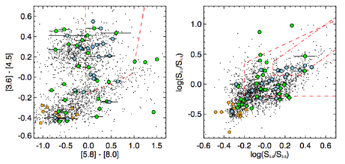
Figure 17.— IRAC color-color diagrams. Left: $[3.6]-[4.5]$ versus $[5.8]-[8.0]$ color-color diagram and the corresponding AGN selection wedge (red dashed line) from Stern et al. (2005). Right: log(S${}_{8.0}/$S_4.5) versus log($S_{5.8}/$S_3.6) color-color diagram and its corresponding AGN selection wedge (red dashed line) from Lacy et al. (2004). The revised AGN selection criteria from Donley et al. (2012) is also plotted in red dash-dotted line. $3.6\mu$m and $4.5\mu$m photometry is from SEDS and $5.8\mu$m and $8.0\mu$m photometry is from SpUDS. We only plot sources with S/N $>3$ in all four IRAC bands. Sources with CLASS_STAR $>0.98$ are shown by small orange dots, X-ray point sources from Ueda et al. (2008) and radio sources from Simpson et al. (2006) by large blue and green dots respectively. Error bars are only shown for X-ray and radio sources for clarity.

Figure 18.— Distribution of the photometric redshifts for galaxies (with flag $=0$) in the CANDELS UDS catalog. Several peaks in the redshift distribution e.g. at $z\sim 0.42$, $0.64$, $0.72$, $1.0$ and $1.62$ (dotted vertical lines) confirm the presence of galaxy groups and clusters in the field. The distribution of the spectroscopic redshifts available in the UDS catalog is shown by the filled gray histogram (multiplied by a factor $10$ for visibility).

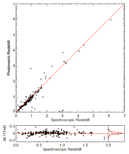
Figure 19.— Top: Comparison between photometric and spectroscopic redshifts for galaxies with available spectroscopic redshift in the UDS catalog. Bottom: Difference $\Delta$$z$ / ($1+z_{spec}$) where $\Delta$$z=z_{spec}-z_{phot}$ restricted for galaxies with $z_{spec}<2$. The right inset shows the distribution of this difference (solid histogram; bin $=0.01$) with a Gaussian distribution with a standard deviation $\sigma=0.022$ overlaid (red curve).

7.4. Photometric redshifts

Intense work is currently being done within the CANDELS team to derive robust photometric redshifts and stellar mass estimates for all sources in the CANDELS multiwavelength catalogs. Dahlen et al. (in prep.) summarize the CANDELS team efforts to (i) compare photometric redshift and mass estimates from different codes ($13$ in total) (ii) assess how well codes manage to recover the redshifts of objects with known spectroscopic redshift and (iii) determine how well codes reproduce stellar masses of simulated galaxies. The final goal is to converge to one unique and optimal photometric redshift and stellar mass estimates recipe that is to be adopted for all CANDELS multiwavelength catalogs.

Photometric redshifts and stellar masses derived from the present UDS multiwavelength catalog will be presented in an upcoming paper. In this section, we make use of one of the $13$ codes presented in Dahlen et al. in prep, namely zphot (Giallongo et al., 1998) as a first test of the photometry of the present catalog. zphot is a $\chi^{2}$-minimization procedure that finds the best-fitting template to the observed colors of a source out of a spectral library of galaxies. The spectral library was built using PEGASE 2.0 models (Fioc & Rocca-Volmerange, 1997). We refer to Grazian et al. (2006) and references therein for further details on zphot.

We first run zphot on sources with available spectroscopic redshifts, derive ‘flux corrections’ i.e. small shifts to be applied to the photometry in order to better match the galaxy templates and then run zphot on the full catalog.

Figure 18 shows the distribution of photometric redshifts for all sources with flag $=0$ in the UDS catalog. A series of peaks in redshifts is observed, suggesting the CANDELS UDS field contains a number of galaxy groups/clusters. We refer to Galametz et al. in prep. for a more detailed study of galaxy overdensities in the UDS. We will just note that two structures were already known in the CANDELS UDS field: a galaxy cluster at $z\sim 0.65$ (Geach et al., 2007, see also Figure 7) and one of the highest redshift galaxy clusters known to date at $z=1.62$ (Papovich et al., 2010, 2012; Tanaka et al., 2010), which are both clearly visible in the photometric redshift distribution.

A comparison between photometric and spectroscopic redshifts is shown in Figure. 19. The quality of the photometric redshifts is excellent. We further study the distribution of the relative difference $z_{spec}-z_{phot}$ / ($1+z_{spec}$). Its central peak can be cleanly fit by a tight Gaussian with an average scatter of $0.022$. However, a large majority of the sources with a spectroscopic redshift in the UDS catalog are AGN and the reliability derived from these sources may not reflect the one of the full catalog, especially for normal faint galaxies.

8. Summary

$\bullet$ The UDS catalog is based on public data including the CANDELS data from HST (WFC3 $F125W$ and $F160W$ and ACS $F606W$ and $F814W$), $u$-band data from CFHT/Megacam, $B$, $V$, $R_{c}$, $i^{\prime}$ and $z^{\prime}$ bands data from Subaru/Suprime-Cam, $Y$ and $K_{s}$ bands data from VLT/HAWK-I, $J$, $H$ and $K$ bands data from UKIDSS (Data Release 8), and Spitzer/IRAC data ($3.6$, $4.5$ from SEDS, $5.8$ and $8.0\mu$m from SpUDS).

$\bullet$ The UDS catalog is based on a source detection in the CANDELS WFC3 $F160W$ image using a slightly modified version of SExtractor. Two detection modes (‘cold’ and ‘hot’) were used (and then merged) to optimally detect and extract all sources ranging from the largest, most extended, and brightest ones to the faintest and smallest. SExtractor was also used to derive the photometry in the other HST bands. The final catalog contains $35932$ sources over an area of $201.7$ square arcmin.

$\bullet$ Independent catalogs were already publicly available for the Subaru, UKIDSS (although earlier releases) and Spitzer/IRAC data. However, the present catalog not only combines all ultraviolet to mid-infrared bands available in the CANDELS UDS field but also takes advantage of the availability of high-resolution and relatively deep data in the field (i.e., the CANDELS HST data). We have indeed used the a-priori information of the position and morphology of sources measured on the $F160W$ image as priors to derive their photometry in the lower-resolution data with the TFIT software.

$\bullet$ We cross-matched the catalog with existing catalogs of X-ray sources and radio sources and included this information in the catalog.

$\bullet$ We also provided, alongside the photometry, a list of sources with spectroscopic redshifts in a first attempt to combine all spectra available in the CANDELS UDS field. More upcoming spectroscopic campaigns are planned in the next months hopefully improving the current restricted list of publicly available spectra.

$\bullet$ A series of convincing tests was done on the photometry to check for its reliability including band-to-band comparison, validation with models and a preliminary study of the photometric redshifts for sources in the catalog.

$\bullet$ The CANDELS UDS multiwavelength catalog is made publicly available on the CANDELS website, the MAST archive, via the on-line version of the article, the Centre de Données astronomiques de Strasbourg (CDS) as well as in the Rainbow Database.

Appendix A Appendix A: SExtractor cold and hot detection modes

The cold mode is optimized for the detection of the brighter and more extended objects. We therefore adopt a relatively large smoothing filter (tophat_9.0_9x9.conv) to include sub-clumps of large galaxies within the same galaxy. The hot mode is optimized to detect the fainter sources and we therefore use a lower detection threshold, a larger deblending and a smaller smoothing filter. Intensive tests and visual inspection were made to optimize these parameters to the CANDELS UDS $F160W$ data. We thoroughly tweaked these parameters to avoid any discontinuity between the cold and the hot mode photometry, especially at the faint end when the cold and hot mode start to be merged by the cold + hot routine. Figure 20 shows the agreement in photometry between the two extraction modes for sources detected in both catalogs.

# SExtractor parameter file
# Differences between the two modes are marked in bold following the scheme ‘Cold / Hot’

#———- Catalog ———-
CATALOG_TYPE ASCII_HEAD
PARAMETERS_NAME file.param
CATALOG_NAME HST.cat
#———- Extraction ———-
DETECT_TYPE CCD
FLAG_TYPE OR
DETECT_MINAREA 5.0 / 10.0
DETECT_THRESH 0.75 / 0.7
ANALYSIS_THRESH 5.0 / 0.7
FILTER Y
FILTER_NAME (cold) tophat_9.0_9x9.conv
FILTER_NAME (hot) gauss_4.0_7x7.conv
DEBLEND_NTHRESH 16 / 64
DEBLEND_MINCONT 0.0001 / 0.001
CLEAN Y
CLEAN_PARAM 1.0
MASK_TYPE CORRECT
#———- Photometry ———-
GAIN HST.gain
MAG_ZEROPOINT HST.zp
PHOT_FLUXFRAC 0.2, 0.5, 0.8
PHOT_APERTURES 1.47, 2.08, 2.94, 4.17, 5.88, 8.34, 11.79, 16.66, 23.57, 33.34, 47.13
PHOT_AUTOPARAMS 2.5, 3.5
SATUR_LEVEL 120.0 / 3900.0
PIXEL_SCALE 0.060
MAG_GAMMA 4.0
#———-Star/Galaxy Separation ———-
SEEING_FWHM 0.18
STARNNW_NAME default.nnw
#———- Background ———-
BACK_SIZE 256 / 128
BACK_FILTERSIZE 9 / 5
BACKPHOTO_TYPE LOCAL
BACKPHOTO_THICK 100 / 48
#———- Weight/Flag Image ———-
#WEIGHT_TYPE MAP_RMS
#WEIGHT_IMAGE HST.rms.fits
WEIGHT_THRESH 10000.0, 10000.0
FLAG_IMAGE FlagH.fits
#———- Memory ———-
MEMORY_OBJSTACK 4000
MEMORY_PIXSTACK 400000
MEMORY_BUFSIZE 5000

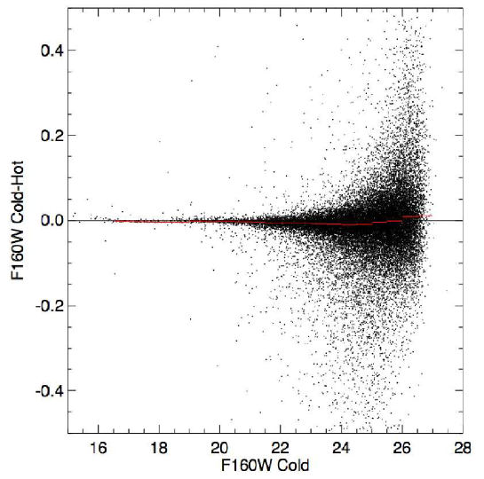
Figure 20.— Offset in photometry for sources detected in both cold and hot modes (with the $\sigma$-clipped mean offset shown in red).

Appendix B Appendix B: Notes on the multiwavelength catalog

Catalog columns:
# ID (1)
# R.A. (deg) (2)
# Dec. (deg) (3)
# F160W Limiting magnitude (4)
# Flag (5)
# CLASS_STAR (6)
# Flux_u_cfht (7)
# Fluxerr_u_cfht (8)
# Flux_B_subaru (9)
# Fluxerr_B_subaru (10)
# Flux_V_subaru (11)
# Fluxerr_V_subaru (12)
# Flux_R_subaru (13)
# Fluxerr_R_subaru (14)
# Flux_i_subaru (15)
# Fluxerr_i_subaru (16)
# Flux_z_subaru (17)
# Fluxerr_z_subaru (18)
# Flux_F606W_hst (19)
# Fluxerr_F606W_hst (20)
# Flux_F814W_hst (21)
# Fluxerr_F814W_hst (22)
# Flux_F125W_hst (23)
# Fluxerr_F125W_hst (24)
# Flux_F160W_hst (25)
# Fluxerr_F160W_hst (26)
# Flux_Y_hawki (27)
# Fluxerr_Y_hawki (28)
# Flux_Ks_hawki (29)
# Fluxerr_Ks_hawki (30)
# Flux_J_ukidss_DR8 (31)
# Fluxerr_J_ukidss_DR8 (32)
# Flux_H_ukidss_DR8 (33)
# Fluxerr_H_ukidss_DR8 (34)
# Flux_K_ukidss_DR8 (35)
# Fluxerr_K_ukidss_DR8 (36)
# Flux_ch1_seds (37)
# Fluxerr_ch1_seds (38)
# Flux_ch2_seds (39)
# Fluxerr_ch2_seds (40)
# Flux_ch3_spuds (41)
# Fluxerr_ch3_spuds (42)
# Flux_ch4_spuds (43)
# Fluxerr_ch4_spuds (44)
# Spectroscopic redshift (45)
# Reference (46)

Column description:
The electronic version of the table contains some extra columns including additional SExtractor parameters derived from the $F160W$ image.
$\bullet$ Column #1: ID number of the source in the $F160W$-selected SExtractor catalog.
$\bullet$ Columns # 2-3: Right Ascension and declination of the source (J2000) in the $F160W$ image.
$\bullet$ Column # 4: Limiting magnitude at the position of the source in the $F160W$ image (see Section 3.3 for details).
$\bullet$ Column # 5: Flag. A specific flag coding is used to designate suspicious sources that fall in contaminated regions. A non-contaminated source has a flag of ‘0’. Sources detected by SExtractor at the image edges or on the few artifacts of the $F160W$ image are assigned a flag of ‘2’. It accounts for $230$ sources that are, for a majority of them, not real but that are kept in the catalog to conserve the SExtractor original number of sources. Sources detected on star spikes, halos and the bright stars that produce those spikes and halos themselves have a flag of ‘1’ ($706$ sources). A large fraction of these sources are real but the photometry of these sources — on which the Template-fitting photometry software TFIT run is based (see Section 4) — is contaminated by a neighbor star.
$\bullet$ Column # 6: CLASS_STAR parameter in the $F160W$-selected SExtractor catalog.
$\bullet$ Columns #7-44: Flux densities in $\mu$Jy and uncertainties for the $21$ bands of the catalog. We consistently report values of $-99$ if the source has no data or is strongly contaminated by a star spike in one specific band.
$\bullet$ Column #45: Spectroscopic redshift when available; ‘-99’ otherwise.
$\bullet$ Column #46: Origin of the spectroscopic redshift when available; ‘-99’ otherwise. The coding follows the scheme ‘reference-type’ (no space):

References are coded as follows:
‘Y05’ = Yamada et al. 2005; ‘G07’ = Geach et al. 2007; ‘Si06’ = Simpson et al. 2006; ‘Si12’ = Simpson et al. 2012; ‘Sm08’ = Smail et al. 2008; ‘Ou08’ = Ouchi et al. 2008; ‘V08’ = Vardoulaki et al. 2008; ‘P10’ = Papovich et al. 2010; ‘T10’ = Tanaka et al. 2010; ‘F10’ = Finoguenov et al. 2010; ‘SIP’ = Simpson et al. in prep.; ‘AIP’ = Akiyama et al. in prep.; ‘CIP’ = Cooper et al. in prep.; ‘PIP’ = Pearce et al. in prep.

Source types are coded as follows:
‘NLAGN’ = Narrow-line AGN; ‘BLAGN’ = Broad-line AGN; ‘RadioS’ = Radio Source; ‘RG’ = Radio Galaxy; ‘XRay’ = X-Ray Source; ‘QSO’ = Quasi Stellar Object; ‘LAE’ = Lyman Alpha Emitter; ‘ClusterMemb’ = Cluster member; ‘OPEG’ = Old Passively Evolving Galaxy.

Source types for galaxies in the radio source catalog from Simpson et al. 2006 and X-ray source catalog from Ueda et al. 2008 are coded as ‘RadioS(Si06)’ and ‘XRay(U08)’ respectively (or both for the only source that was detected in radio and X-ray, namely source #24437). Possible (but questionable) counterparts of X-ray and radio sources are indicated by a ‘?’. Two sources falling within $1$ arcsec of the two X-ray extended source candidates (sources #7217 and #9461) are coded as ‘extXRay(U08)’.

References

- Alard (2000) Alard, C. 2000, A&AS, 144, 363
- Alard & Lupton (1998) Alard, C. & Lupton, R. H. 1998, ApJ, 503, 325
- Aniano et al. (2011) Aniano, G. et al. 2011, PASP, 123, 1218
- Barden et al. (2012) Barden, M. et al. 2012, MNRAS, 422, 449
- Barro et al. (2011) Barro, G. et al. 2011, ApJS, 193, 13
- Bertin (2010) Bertin, E. 2010, in Astrophysics Source Code Library, record ascl:1010.068, 10068
- Bertin & Arnouts (1996) Bertin, E. & Arnouts, S. 1996, A&AS, 117, 393
- Cirasuolo et al. (2010) Cirasuolo, M. et al. 2010, MNRAS, 401, 1166
- Daddi et al. (2004) Daddi, E. et al. 2004, ApJ, 617, 746
- de Santis et al. (2007) de Santis, C. et al. 2007, New Astron., 12, 271
- Donley et al. (2012) Donley, J. L. et al. 2012, ApJ, 748, 142
- Dye et al. (2006) Dye, S. et al. 2006, MNRAS, 372, 1227
- Fazio et al. (2004) Fazio, G. G. et al. 2004, ApJS, 154, 39
- Finoguenov et al. (2010) Finoguenov, A. et al. 2010, MNRAS, 403, 2063
- Fioc & Rocca-Volmerange (1997) Fioc, M. & Rocca-Volmerange, B. 1997, A&A, 326, 950
- Furusawa et al. (2008) Furusawa, H. et al. 2008, ApJS, 176, 1
- Geach et al. (2007) Geach, J. E. et al. 2007, MNRAS, 381, 1369
- Giallongo et al. (1998) Giallongo, E. et al. 1998, AJ, 115, 2169
- Giavalisco et al. (2004) Giavalisco, M. et al. 2004, ApJ, 600, L93
- Gorjian et al. (2008) Gorjian et al. 2008, ApJ, 679
- Gray et al. (2009) Gray, M. E. et al. 2009, MNRAS, 393, 1275
- Grazian et al. (2006) Grazian, A. et al. 2006, A&A, 449, 951
- Grogin et al. (2011) Grogin, N. A. et al. 2011, ApJS, 197, 35
- Gunn & Stryker (1983) Gunn, J. E. & Stryker, L. L. 1983, ApJS, 52, 121
- Koekemoer et al. (2011) Koekemoer, A. M. et al. 2011, ApJS, 197, 36
- Krist (1995) Krist, J. 1995, in Astronomical Society of the Pacific Conference Series, Vol. 77, Astronomical Data Analysis Software and Systems IV, ed. R. A. Shaw, H. E. Payne, & J. J. E. Hayes, 349
- Lacy et al. (2004) Lacy, M. et al. 2004, ApJS, 154, 166
- Laidler et al. (2007) Laidler, V. G. et al. 2007, PASP, 119, 1325
- Lawrence et al. (2007) Lawrence, A. et al. 2007, MNRAS, 379, 1599
- Lee et al. (2012) Lee, K.-S. et al. 2012, ApJ, 752, 66
- Lonsdale et al. (2003) Lonsdale, C. J. et al. 2003, PASP, 115, 897
- Ouchi et al. (2008) Ouchi, M. et al. 2008, ApJS, 176, 301
- Papovich et al. (2001) Papovich, C., Dickinson, M., & Ferguson, H. C. 2001, ApJ, 559, 620
- Papovich et al. (2010) Papovich, C. et al. 2010, ApJ, 716, 1503
- Papovich et al. (2012) —. 2012, ApJ, 750, 93
- Pérez-González et al. (2008) Pérez-González et al. 2008, ApJ, 675, 234
- Santini et al. (2009) Santini, P. et al. 2009, A&A, 504, 751
- Santini et al. (2012) —. 2012, A&A, 538, A33
- Simpson et al. (2006) Simpson, C. et al. 2006, MNRAS, 372, 741
- Simpson et al. (2012) —. 2012, MNRAS, 421, 3060
- Smail et al. (2008) Smail, I. et al. 2008, MNRAS, 389, 407
- Stern et al. (2000) Stern, D., Djorgovski, S. G., Perley, R. A., de Carvalho, R. R., & Wall, J. V. 2000, AJ, 119, 1526
- Stern et al. (2005) Stern, D. et al. 2005, ApJ, 631, 163
- Tanaka et al. (2010) Tanaka, M., Finoguenov, A., & Ueda, Y. 2010, ApJ, 716, L152
- Ueda et al. (2008) Ueda, Y. et al. 2008, ApJS, 179, 124
- van Breukelen et al. (2007) van Breukelen, C. et al. 2007, MNRAS, 382, 971
- van der Wel et al. (2012) van der Wel, A. et al. 2012, ApJS, 203, 24
- Vardoulaki et al. (2008) Vardoulaki, E. et al. 2008, MNRAS, 387, 505
- Yamada et al. (2005) Yamada, T. et al. 2005, ApJ, 634, 861